Influence of variable fluid properties on mixed convective Darcy–Forchheimer flow relation over a surface with Soret and Dufour spectacle

Shuguang Li; Muhammad Ijaz Khan; Shahid Ali; Sami Ullah Khan; Saja Abdulrahman Althobaiti; Ilyas Khan; Faris Alqurashi; Mohamed Kchaou

doi:10.1515/phys-2024-0010

Article Open Access

Influence of variable fluid properties on mixed convective Darcy–Forchheimer flow relation over a surface with Soret and Dufour spectacle

Shuguang Li , Muhammad Ijaz Khan , Shahid Ali , Sami Ullah Khan , Saja Abdulrahman Althobaiti , Ilyas Khan , Faris Alqurashi and Mohamed Kchaou

Published/Copyright: April 13, 2024

Published by

Become an author with De Gruyter Brill

Submit Manuscript Author Information Explore this Subject

From the journal Open Physics Volume 22 Issue 1

Abstract

The thermo-diffusion applications of nanofluid subject to variable thermal sources have been presented. The significance of Darcy–Forchheimer effects is attributed. The flow comprises the mixed convection and viscous dissipation effects. Furthermore, the variable influence of viscosity, thermal conductivity, and mass diffusivity is treated to analyze the flow. The analysis of problem is referred to convective mass and thermal constraints. The analytical simulations are proceeded with homotopy analysis method. The convergence region is highlighted. Novel physical contribution of parameters is visualized and treated graphically. It is noted that larger Brinkman number leads to improvement in heat transfer. The concentration pattern boosted due to Soret number. The wall shear force enhances with Hartmann number and variable thermal conductivity coefficient.

Keywords: Darcy–Forchheimer model; Soret and Dufour phenomenon; convective temperature and concentration constraints; variable transport characteristics

1 Introduction

The nanomaterials are treated as an improved source of energy as a liquid in different industrial processes. The decomposition of nanofluids preserves peak thermal concavity and other features. Various applications of nanomaterials are observed in energy systems, chemical reactions, nuclear systems, high-energy physics, radiative phenomenon, etc. Different studies are performed by many researchers for nanofluids. Wang et al. [1] observed the graphene nanoparticles to boost the performances of engine oil with additional melting phenomenon. The ciliated wavy surface flow comprising the nanofluid endorsing the physiological properties was observed by Fuzhang et al. [2]. Imtiaz et al. [3] developed the understanding of magnetic dipole for nanofluid problem with diverse thermal properties. Wang et al. [4] presented the reflection of solar energy performances with nanoparticle applications. Jayadevamurthy et al. [5] emphasized toward the bioconvective phenomenon due to hybrid nanofluid in rotating systems. Wang et al. [6] observed the natural convective nanofluid flow under the role of chemotaxis phenomenon. Li et al. [7,8,9,10] explored the fluid flow behavior in the presence of various boundary constraints.

Thermo-diffusion, also known as the Soret effect, is a process where solutes are transported in a medium due to a thermal gradient. Most solutes have positive coefficients, indicating that they will diffuse down the thermal gradient, away from the heat source. However, some solutes have negative coefficients and may move up the gradient. The Soret coefficients for various solutes can be found in the study by de Marsily et al. [11]. The importance of thermo-diffusion in the disposal of heat-emitting waste in pelagic silts has been investigated by Thornton and Seyfried [12]. It was noted that the thermo-diffusion plays a significant role in this process. Idowu and Falodun [13] claimed the vertical flow due to thermo-diffusion transport under the Newtonian heating. Javed et al. [14] evaluated the Dufour consequences for numerically treated viscoelastic fluid. Li et al. [15] highlighted the Soret and Dufour appliances for optimized flow. Suchana et al. [16] visualized the multi wall carbon nanotubes-H₂O decomposition in an L-shaped configuration. The Carreau nanofluid with Soret interaction was determined by Salahuddin et al. [17]. Mng'ang'a and Richard Onyango [18] examined the Couette flow due to Jeffrey fluid via inclined channel. Yang et al. [19] and Sun et al. [20] investigated heat flow via 3D-printed thermal meta-materials and shear-thickening fluids based on carbon fiber and silica nanocomposite, respectively.

The study of fluid flow through porous saturated spaces is crucial in various fields such as geophysics, petroleum engineering, industrial geophysics, geothermal operations, soil sciences, packed filters, and ion-exchange columns. Porous media consist of tiny pores through which fluids can be absorbed or injected. These media find applications in energy storage, oil filtration, and thermal receivers. The Darcy law is associated with the applications of porous media in the absence of inertial forces [21,22,23,24,25]. However, this law has limitations in validating low velocity ranges and small porosity spaces. To address this issue, the non-Darcian porous medium, known as the Darcy–Forchheimer law, provides a generalized approach to studying porous spaces, even at low porosity levels. This law successfully describes inertial features, variable porous effects, and boundary impacts. In recent studies, researchers have been exploring the application of the Darcy–Forchheimer model to porous medium flow problems. Ullah et al. [26] investigated the influence of lip on rotating disk flow with nanoparticles using this model. Siddiqui et al. [27] numerically focused on the Casson particles and optimized the determination using the Darcy–Forchheimer model. Saini et al. [28] discussed the modified Darcy contribution for the Jeffrey fluid in porous space with cylindrical particles. Alzahrani and Khan [29] investigated the impact of activation energy on three-dimensional Darcy–Forchheimer flow patterns. Li et al. [40] examined that the unsteady fluid flow and heat transport subject to generalized lie similarity transformations and thermal radiation.

The objective of present continuation is to analyze the thermo-diffusion mixed convection flow of nanofluid comprising the variable thermal sources. The novel features of current work are:

A mixed convection flow of nanofluid with variable viscosity endorsing by moving stretched surface is analyzed,
The flow is subject to significance of Darcy–Forchheimer phenomenon,
The viscous dissipated impact is utilized,
The Soret and Dufour features are contributed,
The dealing of heat transfer is preserved under the assumptions of variable thermal conductivity,
The objective of nanofluid concentration is attained with chemical reaction outcomes,
Both mass and heat fluctuated assessment are inspected with convective transport constraints,
Computational results for modeled problem were computed via homotopy analysis method (HAM) [30,31,32].

It is remarked that different studies are recently summarized for studying various aspects of nanomaterials. However, analysis for Darcy–Forchheimer flow of nanofluid with variable thermal features and thermo-diffusion effects has not been focused yet. Current model aims to fulfill this research gap. A physical attribution of problem is observed.

2 Formulation of problem

In this study, we investigate the two-dimensional, incompressible, steady mixed convective flow of a viscous fluid over a movable surface in the presence of Soret and Dufour effects. The flow takes place in a Darcy–Forchheimer porous medium with variable transport characteristics, including thermal conductivity, viscosity, and diffusivity. The temperature and concentration distributions are determined, considering the effects of thermophoresis and Brownian diffusion. Additionally, convective boundary conditions for temperature and concentration are applied at the surface boundary. The surface is stretched having velocity ( u w ( x ) = a x ) with a > 0 . A constant magnetic is applied with constant strength ( B 0 ). The physical representation of the flow is shown in Figure 1.

Figure 1

Flow sketch.

Governing equations are as follows [33,34,35,36]:

(1) ∂ u ∂ x + ∂ v ∂ y = 0 ,

(2) ρ f u ∂ u ∂ x + v ∂ u ∂ y = ∂ ∂ y μ ( T ) ∂ u ∂ y − σ f B 0 2 u − μ f k p u − ρ f F u 2 + g ∗ ρ f β ∗ ( T − T ∞ ) + g ∗ ρ f β ∗ ∗ ( C − C ∞ ) ,

(3) u ∂ T ∂ x + v ∂ T ∂ y = 1 ( ρ c p ) f ∂ ∂ y k ( T ) ∂ T ∂ y + τ D b ∂ C ∂ y ∂ T ∂ y + D T T ∞ ∂ T ∂ y 2 + σ f B 0 2 ( ρ c p ) f u 2 + D b k T ( c p ) f C s ∂ 2 C ∂ y 2 ,

(4) u ∂ C ∂ x + v ∂ C ∂ y = D B ( C ) ∂ 2 C ∂ y 2 + D T T ∞ ∂ 2 T ∂ y 2 + D b k T T m ∂ 2 T ∂ y 2 − k r 2 ( C − C ∞ ) ,

(5) u = a x , v = 0 , − k f ∂ T ∂ y = h f ( T w − T ) , − D B ∂ C ∂ y = h w ( C w − C ) at y = 0 u → 0 , T → T ∞ , C → C ∞ as y → ∞ .

Here, ( u , v ) signify the velocity components, D b Brownian motion coefficient, T m mean fluid temperature, μ f dynamic viscosity, T w wall temperature, σ f electrical conductivity, β ∗ thermal expansion coefficient, ( x , y ) Cartesian coordinates, h f heat transfer rate, g ∗ gravity, ρ f density of fluid, β ∗ ∗ the solutal expansion coefficient, T temperature, F = C b k p non-uniform inertia coefficient, ( c p ) f specific heat, l characteristics length, k ∗ mean absorption coefficient, k r 2 reaction rate, τ the ratio of heat capacitance, k p porous space coefficient, k T thermal diffusion ratio, T ∞ ambient temperature, h w mass transfer rate, σ ∗ Stefan–Boltzmann constant, C s concentration susceptibility, D T thermophoresis coefficient, k f thermal conductivity, C the concentration, C w wall concentration, and C ∞ ambient concentration. Here, variable fluid behaviors are defined as [37,38]:

(6) μ ( T ) = μ f 1 + ∈ 1 T − T ∞ T w − T ∞ ,

(7) k ( T ) = k f 1 + ∈ 2 T − T ∞ T w − T ∞ ,

(8) D B ( C ) = D b 1 + ∈ 3 C − C ∞ C w − C ∞ .

Using transformations [39]

(9) u = x ∂ f ( ξ , η ) ∂ η , v = − a ν f f ( ξ , η ) + ξ ∂ f ( ξ , η ) ∂ ξ , θ ( ξ , η ) = T − T ∞ T w − T ∞ ϕ ( ξ , η ) = C − C ∞ C w − C ∞ , ξ = x l , η = a ν f y .

One can found that

(10) ( 1 + ∈ 1 θ ) ∂ 3 f ∂ η 3 + ∈ 1 ∂ θ ∂ η ∂ 2 f ∂ η 2 + f ∂ 2 f ∂ η 2 + ξ ∂ f ∂ ξ ∂ 2 f ∂ η 2 − ∂ f ∂ η 2 − ξ ∂ 2 f ∂ ξ ∂ η ∂ f ∂ η − M ∂ f ∂ η − λ ∂ f ∂ η − Fr ξ ∂ f ∂ η 2 + β t ξ ( θ + β c φ ) = 0 ,

(11) ( 1 + ∈ 2 θ ) ∂ 2 θ ∂ η 2 + ∈ 2 ∂ θ ∂ η 2 + Pr ξ ∂ f ∂ ξ ∂ θ ∂ η + Pr f ∂ θ ∂ η − Pr ξ ∂ θ ∂ ξ ∂ f ∂ η + PrNb ∂ θ ∂ η ∂ ϕ ∂ η + Pr Nt ∂ θ ∂ η 2 + M Br ξ 2 ∂ f ∂ η 2 + Pr Du ∂ 2 ϕ ∂ η 2 = 0 ,

(12) ( 1 + ∈ 3 ϕ ) ∂ 2 ϕ ∂ η 2 + ∈ 3 ∂ ϕ ∂ η 2 + Sc f ∂ ϕ ∂ η + Sc ξ ∂ f ∂ ξ ∂ ϕ ∂ η − Sc ξ ∂ ϕ ∂ ξ ∂ f ∂ η + Nt Nb ∂ 2 θ ∂ η 2 + ScSr ∂ 2 θ ∂ η 2 − γ Sc ϕ = 0 ,

(13) ∂ f ( ξ , 0 ) ∂ η = 1 , f ( ξ , 0 ) = − ξ ∂ f ( ξ , 0 ) ∂ ξ , ∂ θ ( ξ , 0 ) ∂ η = − β 1 ( 1 − θ ( 0 ) ) ∂ ϕ ( ξ , 0 ) ∂ η = − β 2 ( 1 − ϕ ( 0 ) ) ∂ f ( ξ , ∞ ) ∂ η = 0 , θ ( ξ , ∞ ) = 0 , ϕ ( ξ , ∞ ) = 0 .

where ∈ 1 denotes the variable viscosity parameter, Pr = ν f α f the Prandtl number, Sc = ν f D b the Schmidt number, Ec = u 0 2 l 2 ( c p ) f ( T w − T ∞ ) the Eckert number, M = σ f B 0 2 a ρ f the Hartmann number, β t = g ∗ β ∗ ( T w − T ∞ ) a 2 l the mixed convection variable, γ = k r 2 a the reaction variable, Sr = D b k T ( T w − T ∞ ) T m ( C w − C ∞ ) ν f the Soret number, β c = β ∗ ∗ ( C w − C ∞ ) β ∗ ( T w − T ∞ ) the buoyancy ratio parameter, ∈ 2 variable thermal conductivity parameter, ∈ 3 variable mass diffusivity parameter, Nt = τ D T ( T w − T ∞ ) T ∞ ν f thermophoresis variable, Nb = τ D b ( C w − C ∞ ) ν f Brownian motion variable, Du = D b k T ( C w − C ∞ ) ( c p ) f C s ν f the Dufour number, β 1 = h f k f a ν f thermal Biot number, Fr = C b k p l Darcy–Forchheimer number, Br ( = Pr Ec ) Brinkman number, β 2 = h w D b a ν f solutal Biot number, and λ = ν f a k p porosity parameter.

3 Engineering quantities

3.1 Drag force coefficient

Mathematically,

(14) C f , x = τ x y ρ f u w 2 ,

Shear stress τ x y is

(15) τ x y = μ ( T ) ∂ u ∂ y y = 0 ,

Dimensionless form

(16) C f x Re x 1 / 2 = ( 1 + ∈ 1 θ ( 0 ) ) f ″ ( 0 ) .

3.2 Nusselt number

Mathematically, it is given as

(17) Nu x = x q w k f ( T w − T ∞ ) ,

Heat flux q w satisfies

(18) q w = − k ( T ) ∂ T ∂ y y = 0 ,

Dimensionless form

(19) Nu x Re x − 1 / 2 = − ( 1 + ∈ 2 θ ( 0 ) ) θ ′ ( 0 ) .

3.3 Sherwood number

Mathematically,

(20) Sh x = x j w ∣ y = 0 D b ( C w − C ∞ ) ,

The heat flux j w is defined as

(21) j w = − D B ( C ) ∂ C ∂ y ,

The dimensionless form is

(22) Sh x Re x − 1 / 2 = − ( 1 + ∈ 3 ϕ ( 0 ) ) ϕ ′ ( 0 ) .

Here, R e x = u w x ν , indicates the local Reynolds number.

4 Solution development

4.1 First-order truncation

For the first-order truncation, we suppose that ∂ ( . ) ∂ ξ ( = 0 ) and ∂ ( . ) ∂ η ( = ′ ) in Eqs. (10)–(13).

(23) ( 1 + ∈ 1 θ ) f ‴ + ∈ 1 θ ′ f ″ + f f ″ − f ′ 2 − M f ′ − λ f ′ − Fr ξ f ′ 2 + β t ξ ( θ + β c ϕ ) = 0 ,

(24) ( 1 + ∈ 2 θ ) θ ″ + ∈ 2 θ ′ 2 + Pr f θ ′ + Pr Nb θ ′ ϕ ′ + Pr Nt θ ′ 2 + M Br ξ 2 f ′ 2 + Pr Du ϕ ″ = 0 ,

(25) ( 1 + ∈ 3 ϕ ) ϕ ″ + ∈ 3 ϕ ′ 2 + Sc f ϕ ′ + N t N b θ ″ + ScSr θ ″ − γ Sc ϕ = 0 ,

(26) f ′ ( ξ , 0 ) = 1 , f ( ξ , 0 ) = 0 , θ ′ ( ξ , 0 ) = − β 1 ( 1 − θ ( 0 ) ) ϕ ′ ( ξ , 0 ) = − β 2 ( 1 − ϕ ( 0 ) ) f ′ ( ξ , ∞ ) = 0 , θ ( ξ , ∞ ) = 0 , ϕ ( ξ , ∞ ) = 0 .

4.2 Second-order truncation

For the second- order truncation, we suppose that ∂ f ∂ ξ = p , ∂ 2 f ∂ ξ ∂ η = ∂ p ∂ η , ∂ 3 f ∂ ξ ∂ η 2 = ∂ 2 p ∂ η 2 , ∂ θ ∂ ξ = q , ∂ 2 θ ∂ ξ ∂ η = ∂ q ∂ η , ∂ φ ∂ ξ = g , and ∂ 2 φ ∂ ξ ∂ η = ∂ g ∂ η , in Eqs. (10)–(13). We have

(27) ( 1 + ∈ 1 θ ) ∂ 3 f ∂ η 3 + ∈ 1 ∂ θ ∂ η ∂ 2 f ∂ η 2 + f ∂ 2 f ∂ η 2 + ξ p ∂ 2 f ∂ η 2 − ∂ f ∂ η 2 − ξ ∂ p ∂ η ∂ f ∂ η − M ∂ f ∂ η − λ ∂ f ∂ η − Fr ξ ∂ f ∂ η 2 + β t ξ ( θ + β c ϕ ) = 0 ,

(28) ( 1 + ∈ 2 θ ) ∂ 2 θ ∂ η 2 + ∈ 2 ∂ θ ∂ η 2 + Pr ξ p ∂ θ ∂ η + Pr f ∂ θ ∂ η − Pr ξ q ∂ f ∂ η + Pr Nb ∂ θ ∂ η ∂ ϕ ∂ η + Pr Nt ∂ θ ∂ η 2 + M Br ξ 2 ∂ f ∂ η 2 + Pr Du ∂ 2 ϕ ∂ η 2 = 0 ,

(29) ( 1 + ∈ 3 ϕ ) ∂ 2 ϕ ∂ η 2 + ∈ 3 ∂ φ ∂ η 2 + Sc f ∂ ϕ ∂ η + Sc ξ p ∂ ϕ ∂ η − Sc ξ g ∂ f ∂ η + Nt Nb ∂ 2 θ ∂ η 2 + ScSr ∂ 2 θ ∂ η 2 − γ Sc ϕ = 0 ,

(30) ∂ f ( ξ , 0 ) ∂ η = 1 , f ( ξ , 0 ) = − ξ p , ∂ θ ( ξ , 0 ) ∂ η = − β 1 ( 1 − θ ( 0 ) ) ∂ ϕ ( ξ , 0 ) ∂ η = − β 2 ( 1 − ϕ ( 0 ) ) ∂ f ( ξ , ∞ ) ∂ η = 0 , θ ( ξ , ∞ ) = 0 , ϕ ( ξ , ∞ ) = 0 .

Now in Eqs. (27)–(30) derivative with respect to “ ξ ” and the terms having ∂ p ∂ ξ , ∂ 2 p ∂ ξ ∂ η , ∂ 3 p ∂ ξ ∂ η 2 , ∂ q ∂ ξ , ∂ 2 q ∂ ξ ∂ η , ∂ g ∂ ξ , ∂ 2 g ∂ ξ ∂ η are vanished and ∂ ( ⋅ ) ∂ η denoting by prime.

(31) ( 1 + ∈ 1 θ ) p ‴ + ∈ 1 q f ‴ + ε 1 q ′ f ″ + ε 1 θ ′ p ″ + 2 p f ″ + f p ″ + ξ p p ″ − 3 f ′ p ′ − ξ p ′ 2 − M p ′ − λ p ′ − Fr f ′ 2 − 2 Fr f ′ p ′ − β t ξ 2 ( θ + β c ϕ ) + β t ξ ( q + β c g ) = 0 ,

(32) ( 1 + ∈ 2 θ ) q ″ + ∈ 2 q θ ″ + 2 ∈ 2 θ ′ q ′ + 2 Pr p θ ′ + Pr f q ′ − Pr q f ′ − Pr ξ p ′ q + Pr ξ p q ′ + Pr Nb θ ′ g ′ + Pr Nb q ′ ϕ ′ + 2 Pr Nt θ ′ q ′ + 2 M Br ξ f ′ 2 + 2 M Br ξ 2 f ′ p ′ + Pr Du g ″ = 0 ,

(33) ( 1 + ∈ 3 ϕ ) g ″ + ∈ 3 g ϕ ″ + 2 ∈ 3 ϕ ′ g ′ + Sc p ϕ ′ + Sc f g ′ − Sc g f ′ − Sc ξ p ′ g + Sc ξ p g ′ Nt Nb q ″ + ScSr q ″ − γ Sc g = 0 ,

(34) p ′ ( ξ , 0 ) = 0 , p ( ξ , 0 ) = 0 , q ′ ( ξ , 0 ) = β 1 q ( ξ , 0 ) g ′ ( ξ , 0 ) = β 2 g ( ξ , 0 ) p ′ ( ξ , ∞ ) = 0 , q ( ξ , ∞ ) = 0 , g ( ξ , ∞ ) = 0 .

5 HAM

The assessment of problem is presented with the implementation of optimal HAM. HAM scheme is implemented in wide range to different nonlinear problems in era of engineering, biology, sciences, and industrial processes. The motivations for utilizing HAM technique preserve less residual error. The excellent convergence criteria are associated with this method. Defining the initial guesses and linear operators as follows:

(35) f 0 ( η ) = 1 − e − η θ 0 ( η ) = β 1 ( 1 + β 1 ) e − η ϕ 0 ( η ) = β 2 ( 1 + β 2 ) e − η ,

(36) L f = ∂ 3 ∂ η 3 − ∂ ∂ η L θ = ∂ 2 ∂ η 2 − 1 L ϕ = ∂ 2 ∂ η 2 − 1 ,

subject to

(37) L f [ c 0 + c 1 e − η + c 2 e η ] = 0 , L θ [ c 3 e − η + c 4 e η ] = 0 , L ϕ [ c 5 e − η + c 6 e η ] = 0 .

Here, c i ( i = 0 , 1 , 2 , … , 6 ) represents the arbitrary constants.

6 Convergence analysis

The auxiliary parameters ℏ f , ℏ θ , and ℏ ϕ play a significant role in controlling the convergence of solutions. The ℏ -curves are shown in Figure 2. The ranges for meaningful values are − 1.4 ≤ ℏ f ≤ − 0.1 , − 1.3 ℏ θ ≤ − 0.3 , and − 1.3 ≤ ℏ φ ≤ − 0.2 . Various orders of approximation for flow variables are highlighted in Table 1.

$Figure 2 ℏ \hslash -curves.$

Figure 2

ℏ -curves.

Table 1

Various order of approximation for various flow parameters

Order of approximation	‒f″ (0)	θ′	ϕ′ (0)
1	1.172	0.9845	0.9845
8	1.180	0.9119	0.9119
12	1.180	0.8562	0.8354
18	1.180	0.8562	0.8354
22	1.180	0.8562	0.8354
24	1.180	0.8409	0.8264
28	1.180	0.8362	0.8153
30	1.180	0.8362	0.8153

7 Validation of results

Table 2 has been meticulously crafted to provide a solid foundation for validating our current findings by juxtaposing them with previously published results in the existing body of literature. In this analysis, we have focused on comparing the heat transport rate against higher estimations of the Prandtl number, while holding all other parameters constant, and we have specifically referenced the work of Khan et al. [39]. Remarkably, our results exhibit a remarkable concurrence with Wang’s findings, strengthening the credibility of this study.

Table 2

Comparative analysis of heat transport rate with Khan et al. [39]

Pr	Khan et al. [40]	Recent results
0.07	0.065609	0.065612
0.20	0.169115	0.169121
0.70	0.453920	0.453931
2.00	0.911435	0.911439

8 Analysis of results

Physical analysis for observing the profiles of velocity, concentration, and thermal distribution is interpreted. Graphical description of skin friction, solutal transport rate, and Nusselt number for secondary variables is explored.

8.1 Velocity profile

The phenomenon of velocity profile f ′ ( η ) via variable viscosity parameter ∈ 1 is portrayed in Figure 3. An increment in velocity is detected versus higher variable viscosity parameter. The flow Hartmann constant M is sketched in Figure 4. An increment in resistive force is witnessed with variation in magnetic field, which leads to decays velocity. Such results are physically attributed to the role of Lorentz force, which resists the fluid movement. The performance of f ′ ( η ) against porosity constant λ is illustrated in Figure 5. An enhancement in λ leads to upsurges viscous force and so fluid motion decays. Physically, this retarded behavior is due to the permeability of porous medium. The variation of Darcy–Forchheimer constant Fr on f ′ ( η ) is displayed in Figure 6. An enhancing function for velocity change due to Fr is claimed. Physical aspects for this change are the applications of inertial forces.

$Figure 3 f ′ ( η ) f^{\prime} (\eta ) vs ∈ 1 {\in }_{1} .$

Figure 3

f ′ ( η ) vs ∈ 1 .

$Figure 4 f ′ ( η ) f^{\prime} (\eta ) vs M M .$

Figure 4

f ′ ( η ) vs M .

$Figure 5 f ′ ( η ) f^{\prime} (\eta ) vs λ \lambda .$

Figure 5

f ′ ( η ) vs λ .

$Figure 6 f ′ ( η ) f^{\prime} (\eta ) vs Fr \text{Fr} .$

Figure 6

f ′ ( η ) vs Fr .

8.2 Temperature profile

The feature of temperature profile θ ( η ) via thermal Biot number β 1 is shown in Figure 7. In fact, higher β 1 corresponds to generate an additional heat in system that upgrades thermal field. The improvement in profile of θ ( η ) is due to the fact that β 1 is physically attributed to the enhancement in heat transfer coefficient. Figure 8 shows the impact of variable thermal conductivity parameter ∈ 2 on θ ( η ) . The assumptions of variable thermal conductivity are more effective to increase the heat transfer rate. The variation of thermophoresis parameter Nt and Brownian constant Nb on temperature is shown in Figures 9 and 10, respectively. Improvement in θ ( η ) is observed due to both Nt and Nb . Physically, Nt involves the thermophoresis phenomenon, which leads to the movement of fluid liquids in cold surface. Such migration confirmed the improvement in heat transfer. Furthermore, increasing change in θ ( η ) regarding the variation of Nb involves the Brownian movement. In Figure 11, the temperature distribution θ ( η ) is enhanced via the Brinkman number Br . Physically boosting in Br implies a lower distribution to the thermal conduction caused by viscous dissipation, which enlarges the temperature. Figure 12 depicts the magnification of θ ( η ) against the Dufour number Du . Larger approximation of Dufour constant Du corresponds to intensify the thermal distribution. Physically, increasing change in Du leads to enhanced thermal diffusivity because θ ( η ) gets boosted.

$Figure 7 θ ( η ) \theta (\eta ) vs β 1 {\beta }_{1} .$

Figure 7

θ ( η ) vs β 1 .

$Figure 8 θ ( η ) \theta (\eta ) vs ∈ 2 {\in }_{2} .$

Figure 8

θ ( η ) vs ∈ 2 .

$Figure 9 θ ( η ) \theta (\eta ) vs Nt \text{Nt} .$

Figure 9

θ ( η ) vs Nt .

$Figure 10 θ ( η ) \theta (\eta ) vs Nb \text{Nb} .$

Figure 10

θ ( η ) vs Nb .

$Figure 11 θ ( η ) \theta (\eta ) vs Br \text{Br} .$

Figure 11

θ ( η ) vs Br .

$Figure 12 θ ( η ) \theta (\eta ) vs Du \text{Du} .$

Figure 12

θ ( η ) vs Du .

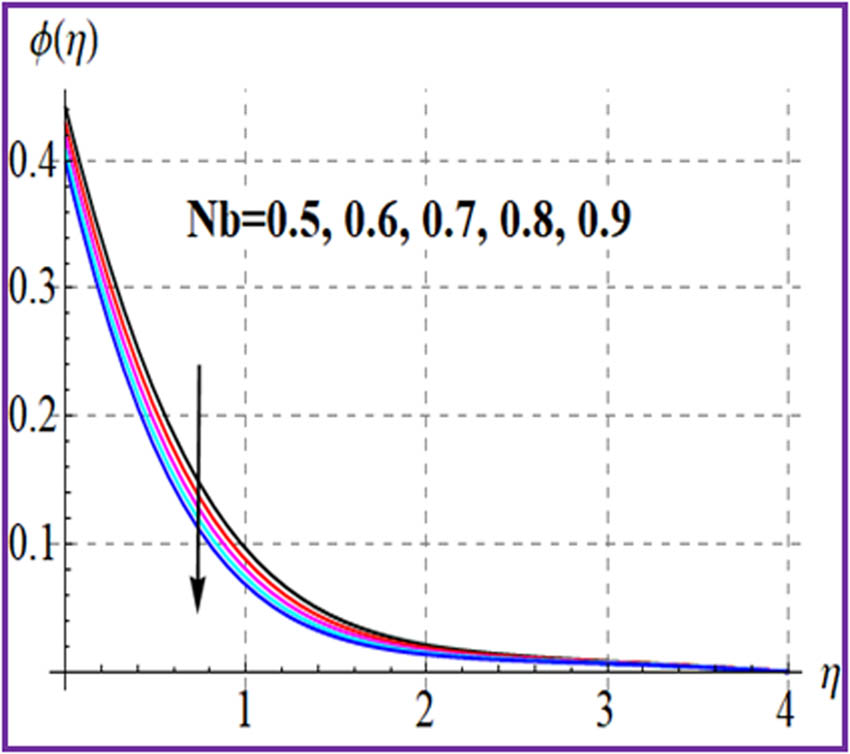
8.3 Concentration profile

Figures 13 and 14 are sketched to show the fluctuation in ϕ ( η ) against Nt and Nb . An improvement in ϕ ( η ) is claimed for Nt , while the reverse change is addressed for Nb . Improvement in ϕ ( η ) is due to thermophoresis phenomenon. Figure 15 demonstrates the impact of variable mass diffusivity coefficient ∈ 3 on ϕ ( η ) . An increment in ∈ 3 leads to an enlargement in ϕ ( η ) . The influence of β 2 on ϕ ( η ) is illustrated in Figure 16. An improvement in concentration distribution via higher β 2 is noted. Concentration trend for the found Soret Sr number is displayed in Figure 17. Clearly, larger values of Soret number Sr lead to enhancement in molar mass diffusivity. Consequently, concentration is increased.

$Figure 13 ϕ ( η ) \phi (\eta ) vs Nt \text{Nt} .$

Figure 13

ϕ ( η ) vs Nt .

$Figure 14 ϕ ( η ) \phi (\eta ) vs Nb \text{Nb} .$

Figure 14

ϕ ( η ) vs Nb .

$Figure 15 ϕ ( η ) \phi (\eta ) vs ∈ 3 {\in }_{3} .$

Figure 15

ϕ ( η ) vs ∈ 3 .

$Figure 16 ϕ ( η ) \phi (\eta ) vs β 2 {\beta }_{2} .$

Figure 16

ϕ ( η ) vs β 2 .

$Figure 17 ϕ ( η ) \phi (\eta ) vs Sr \text{Sr} .$

Figure 17

ϕ ( η ) vs Sr .

8.4 Physical quantities

Graphical description of drag force C f x , solutal transport rate Sh x , and Nusselt number Nu x via secondary variables is interpreted in Figures 18–21. The influence of C f x against M and variable viscosity ∈ 1 variables is deployed in Figure 18. It is noted that drag force has an increasing trend for M and ∈ 1 . Figure 19 is sketched to show the Nu x variation versus the thermal Biot number β 1 and variable conductivity factor ∈ 2 . The heat transport rate has an increasing effect due to β 1 and ∈ 2 . The profile of Sherwood number Sh x has a similar trend for the random variation of Nb and thermophoresis constant Nt and visualized via Figure 20. Figure 21 claims that an increment in solutal transport rate is obtained for β 2 and ∈ 3 .

$Figure 18 C f x {C}_{fx} vs M M and ∈ 1 {\in }_{1} .$

Figure 18

C f x vs M and ∈ 1 .

$Figure 19 Nu x {\text{Nu}}_{x} vs β 1 {\beta }_{1} and ∈ 2 {\in }_{2} .$

Figure 19

Nu x vs β 1 and ∈ 2 .

$Figure 20 Sh x {\text{Sh}}_{x} vs Nt \text{Nt} and Nb \text{Nb} .$

Figure 20

Sh x vs Nt and Nb .

$Figure 21 Sh x {\text{Sh}}_{x} vs β 2 {\beta }_{2} and ∈ 3 {\in }_{3} .$

Figure 21

Sh x vs β 2 and ∈ 3 .

9 Closing remarks

Mixed convective Darcy–Forchheimer flow of nanofluid is studied in the presence of viscous dissipation effects. The formulated problem is solved with optimal homotopy asymptotic method technique. Solution is validated with excellent accuracy. Major results are summarized as:

An improvement in velocity profile is noted for Darcy–Forchheimer parameter and variable viscosity coefficient,
The boosted change is observed in variable thermal conductivity parameter and the Brinkman number,
With the Dufour number and the Biot constant, the heat transfer is sufficiently boosted,
Larger solutal Biot number and variable mass diffusivity lead to an improvement in concentration field,
The variation of wall shear force against the Hartmann number is enhanced for variable viscosity parameter,
An increasing fluctuation of Sherwood number with the Brownian constant shows an increasing function with thermophoresis parameter,
Such results can be further updated by incorporating the entropy generation phenomenon, artificial neural network, and sensitivity analysis.

Acknowledgments

The authors are thankful to the Deanship of Graduate Studies and Scientific Research at University of Bisha for supporting this work through the Fast-Track Research Support Program.

Funding information: The authors state no funding involved.
Author contributions: All authors have accepted responsibility for the entire content of this manuscript and approved its submission.
Conflict of interest: The authors state no conflict of interest.

References

[1] Wang F, Awais M, Parveen R, Alam MK, Rehman S, Shah NA. Melting rheology of three-dimensional Maxwell nanofluid (Graphene-Engine-Oil) flow with slip condition past a stretching surface through Darcy-Forchheimer medium. Results Phys. 2023;51:106647.10.1016/j.rinp.2023.106647Search in Google Scholar

[2] Fuzhang W, Akhtar S, Nadeem S, El-Shafay AS. Mathematical computations for the physiological flow of Casson fluid in a vertical elliptic duct with ciliated heated wavy walls. Waves Random Complex Media. 2022;1–14.10.1080/17455030.2022.2072973Search in Google Scholar

[3] Imtiaz M, Khan MI, Akermi M, Hejazi HA. Understanding the impact of magnetic dipole and variable viscosity on nanofluid flow characteristics over a stretching surface. J Magnetism Magnetic Mater. 2024;589:171613.10.1016/j.jmmm.2023.171613Search in Google Scholar

[4] Wang F, Jamshed W, Ibrahim RW, Abdalla NS, Abd-Elmonem A, Hussain SM. Solar radiative and chemical reactive influences on electromagnetic Maxwell nanofluid flow in Buongiorno model. J Magnetism Magnetic Mater. 2023;576:170748.10.1016/j.jmmm.2023.170748Search in Google Scholar

[5] Jayadevamurthy PG, Rangaswamy NK, Prasannakumara BC, Nisar KS. Emphasis on unsteady dynamics of bioconvective hybrid nanofluid flow over an upward–downward moving rotating disk. Numer Methods Partial Differ Equ. 2024;40(1):e22680.10.1002/num.22680Search in Google Scholar

[6] Wang F, Ahmed A, Khan MN, Ahammad NA, Alqahtani AM, Eldin SM, et al. Natural convection in nanofluid flow with chemotaxis process over a vertically inclined heated surface. Arab J Chem. 2023;16(4):104599.10.1016/j.arabjc.2023.104599Search in Google Scholar

[7] Li S, Imtiaz M, Khan MI, Kumar RN, Akramova KS. Applications of Soret and Dufour effects for Maxwell nanomaterial by convectively heated surface. Numer Heat Transfer, Part A: Appl. 2024;1–5. 10.1080/10407782.2024.2314224.Search in Google Scholar

[8] Li S, Khan MI, Khan SU, Abdullaev S, Mohamed MM, Amjad MS. Effectiveness of melting phenomenon in two phase dusty carbon nanotubes (Nanomaterials) flow of Eyring-Powell fluid: Heat transfer analysis. Chin J Phys. 2023;86:160–9. 10.1016/j.cjph.2023.09.013.Search in Google Scholar

[9] Li S, Rajashekhar C, Nisar KS, Mebarek-Oudina F, Vaidya H, Khan MI, et al. Peristaltic transport of a Ree-Eyring fluid with non-uniform complaint channel: An analysis through varying conditions. ZAMM-J Appl Math Mech/Z für Angew Math und Mechanik. 2023;104(2):e202300073. 10.1002/zamm.202300073.Search in Google Scholar

[10] Li S, Khan MI, Ali F, Abdullaev SS, S Saadaoui HA. Mathematical modeling of mixed convective MHD Falkner-Skan squeezed Sutterby multiphase flow with non-Fourier heat flux theory and porosity. Appl Math Mech-Engl Ed. 2023;44:2005–18.10.1007/s10483-023-3044-5Search in Google Scholar

[11] de Marsily G, Fargue D, Goblet P. How much do we know about coupled processes in the geosphere and their relevance to performance assessment? In Proc. Geoval Symposium, SKI, Stockholm. vol. 2; 1987. p. 475–91.Search in Google Scholar

[12] Thornton EC, Seyfried WE. Chemical and diffusional effects in a thermal gradient: results of recent experimental studies and implications for sub-seabed disposal of nuclear waste. In: Tsang C, Editor. Coupled processes associated with nuclear waste repositories. London: Academic Press; 1985. p. 355–61.Search in Google Scholar

[13] Idowu AS, Falodun BO. Variable thermal conductivity and viscosity effects on non-Newtonian fluids flow through a vertical porous plate under Soret-Dufour influence. Math Comput Simul. 2020;177:358–84.10.1016/j.matcom.2020.05.001Search in Google Scholar

[14] Javed T, Ghaffari A, Majeed A. Numerical investigation on flow of second grade fluid due to stretching cylinder with Soret and Dufour effects. J Mol Liq. 2016;221:878–84.10.1016/j.molliq.2016.06.065Search in Google Scholar

[15] Li S, Khan MI, Rafiq M, Abdelmohsen SAM, Abdullaev SS, Amjad MS. Optimized framework for Darcy-Forchheimer flow with chemical reaction in the presence of Soret and Dufour effects: A shooting technique. Chem Phys Lett. 2023;825:140578.10.1016/j.cplett.2023.140578Search in Google Scholar

[16] Suchana K, Islam MM, Molla MM. Lattice Boltzmann simulation of cross diffusion via Soret and Dufour effects on natural convection of experimental data based MWCNTs-H2O nanofluids in an L-shaped enclosure. Int J Thermofluids. 2024;21:100546.10.1016/j.ijft.2023.100546Search in Google Scholar

[17] Salahuddin T, Awais M, Raza MI. Thermophysical characteristics with natural convective flow of Carreau fluid influencing by Soret and Dufour effects: By using numerical technique. Int J Thermofluids. 2024;21:100589.10.1016/j.ijft.2024.100589Search in Google Scholar

[18] Mng'ang'a J, Richard Onyango E. Joule heating and induced magnetic field on magnetohydrodynamic generalised Couette flow of Jeffrey fluid in an inclined channel with Soret and Dufour effects. Int J Ambient Energy. 2024;45(1):2305328.10.1080/01430750.2024.2305328Search in Google Scholar

[19] Yang S, Zhang Y, Sha Z, Huang Z, Wang H, Wang F, et al. Deterministic manipulation of heat flow via three-dimensional-printed thermal meta-materials for multiple protection of critical components. ACS Appl Mater Interfaces. 2022;14:39354–63.10.1021/acsami.2c09602Search in Google Scholar PubMed

[20] Sun L, Liang T, Zhang C, Chen J. The rheological performance of shear-thickening fluids based on carbon fiber and silica nanocomposite. Phys Fluids. 2023;35:32002.10.1063/5.0138294Search in Google Scholar

[21] de Marsily G, Fargue D, Goblet P. How much do we know about coupled processes in the geosphere and their relevance to performance assessment? In Proc. Geoval Symposium, SKI, Stockholm. vol. 2; 1987. p. 475–91.Search in Google Scholar

[22] Jamet P, Fargue D. Coupled processes in the nearfield. In Proceeding of the Technical Workshop on Near-Field Assessment for High-level Waste, Madrid, Stockholm, Sweden. SKB Technical Rept. vol. 17; 1990. p. 91–59.Search in Google Scholar

[23] Fargue D, Goblet P, Jamet P. Etudes Sous L’angle Thermodynamique des Processus de Transfert Potentials Nondominant des Radionucleides dans la Grosphere, Final Rept. No. LHM/RD/89/52, Prepared for CEC By Ecole Nationale Suprrieure Des Mines de Paris, Centre D’Informatique; 1990.Search in Google Scholar

[24] Thornton EC, Seyfried WE. Chemical and diffusional effects in a thermal gradient: results of recent experimental studies and implications for sub-seabed disposal of nuclear waste. In: Tsang C, Editor. Coupled processes associated with nuclear waste repositories. London: Academic Press; 1985. p. 355–61.10.1016/B978-0-12-701620-7.50030-1Search in Google Scholar

[25] Rahman MU, Haq F, Ghazwani HA, Khan MI, Abduvalieva D, Ali S, et al. Darcy-Forchheimer flow of Prandtl nanofluid with irreversibility analysis and cubic autocatalytic chemical reactions. BioNanoScience. 2023;13:1976–87.10.1007/s12668-023-01212-zSearch in Google Scholar

[26] Ullah MZ, Serra-Capizzano S, Baleanu D. A numerical simulation for Darcy-Forchheimer flow of nanofluid by a rotating disk with partial slip effects. Front Phys. 2020;7:219.10.3389/fphy.2019.00219Search in Google Scholar

[27] Siddiqui BK, Batool S, Malik MY, Hassan QM, Alqahtani AS. Darcy Forchheimer bioconvection flow of Casson nanofluid due to a rotating and stretching disk together with thermal radiation and entropy generation. Case Stud Therm Eng. 2021;27:101201.10.1016/j.csite.2021.101201Search in Google Scholar

[28] Saini AK, Chauhan SS, Tiwari A. Creeping flow of Jeffrey fluid through a swarm of porous cylindrical particles: Brinkman-Forchheimer model. Int J Multiph Flow. 2021;145:103803.10.1016/j.ijmultiphaseflow.2021.103803Search in Google Scholar

[29] Alzahrani F, Khan MI. Applications of Darcy-Forchheimer 3D reactive rotating flow of rate type nanoparticles with non-uniform heat source and sink and activation energy. Chem Phys Lett. 2021;783:139054.10.1016/j.cplett.2021.139054Search in Google Scholar

[30] Liao SJ. A general approach to get series solution of non-similarity boundary-layer flows. Commun Nonlinear Sci Numer Simul. 2009;14:2144–59.10.1016/j.cnsns.2008.06.013Search in Google Scholar

[31] Liao SJ. An optimal homotopy-analysis approach for strongly nonlinear differential equations. Commun Nonlinear Sci Numer Simul. 2010;15:2003–16.10.1016/j.cnsns.2009.09.002Search in Google Scholar

[32] Liao SJ. Homotopy analysis method in nonlinear differential equations. Heidelberg, Germany: Springer; 2012.10.1007/978-3-642-25132-0Search in Google Scholar

[33] Jiang N, Studer E, Podvin B. Physical modeling of simultaneous heat and mass transfer: species interdiffusion, Soret effect and Dufour effect. Int J Heat Mass Transf. 2020;156:119758. 10.1016/j.ijheatmasstransfer.2020.119758.Search in Google Scholar

[34] Jawad M, Majeed AH, Nisar KS, Hamida MBB, Alasiri A, Hassan AM, et al. Numerical simulation of chemically reacting Darcy-Forchheimer flow of Buongiorno Maxwell fluid with Arrhenius energy in the appearance of nanoparticles. Case Stud Therm Eng. 2023;50:103413. 10.1016/j.csite.2023.103413.Search in Google Scholar

[35] Kumar KT, Kalyan S, Kandagal M, Tawade JV, Khan U, Eldin SM, et al. Influence of heat generation/absorption on mixed convection flow field with porous matrix in a vertical channel. Case Stud Therm Eng. 2023;47:103049. 10.1016/j.csite.2023.103049.Search in Google Scholar

[36] Kodi R, Ganteda C, Dasore A, Kumar ML, Laxmaiah G, Hasan MA, et al. Influence of MHD mixed convection flow for Maxwell nanofluid through a vertical cone with porous material in the existence of variable heat conductivity and diffusion. Case Stud Therm Eng. 2023;44:102875. 10.1016/j.csite.2023.102875.Search in Google Scholar

[37] Seddeek MA. Effects of radiation and variable viscosity on a MHD free convection flow past a semi-infinite flat plate with an aligned magnetic field in the case of unsteady flow. Int J Heat Mass Transf. 2002;45:931–5.10.1016/S0017-9310(01)00189-2Search in Google Scholar

[38] Mukhopadhyay S, Layek GC. Effects of thermal radiation and variable fluid viscosity on free convective flow and heat transfer past a porous stretching surface. Int J Heat Mass Transf. 2008;51:2167–78.10.1016/j.ijheatmasstransfer.2007.11.038Search in Google Scholar

[39] Khan SA, Hayat T, Alsaedi A. Bioconvection entropy optimized flow of Reiner-Rivlin nanoliquid with motile microorganisms. Alex Eng J. 2023;79:81–92.10.1016/j.aej.2023.07.069Search in Google Scholar

[40] Li S, Safdar M, Taj S, Bilal M, Ahmed S, Khan MI, et al. Generalized Lie similarity transformations for the unsteady flow and heat transfer under the influence of internal heating and thermal radiation. Pramana J Phys. 2023;97:203.10.1007/s12043-023-02672-4Search in Google Scholar

Received: 2023-12-30

Revised: 2024-02-22

Accepted: 2024-03-11

Published Online: 2024-04-13

This work is licensed under the Creative Commons Attribution 4.0 International License.

Articles in the same Issue

https://doi.org/10.1515/phys-2024-0010

Keywords for this article

Darcy–Forchheimer model; Soret and Dufour phenomenon; convective temperature and concentration constraints; variable transport characteristics

Creative Commons

BY 4.0