Characterizing magnetohydrodynamic effects on developed nanofluid flow in an obstructed vertical duct under constant pressure gradient
-
Syed M. Hussain
 and
Ibrahim Alraddadi
and
Ibrahim Alraddadi

Abstract
This research endeavors to conduct an examination of the thermal characteristics within the duct filled with the copper nanoparticles and water as base fluid. In exhaust systems, like car exhausts, chimneys, and kitchen hoods, duct flows are crucial. These systems safely discharge odors, smoke, and contaminants into the atmosphere after removing them from enclosed places. The study focuses on a laminar flow regime that is both hydrodynamically and thermally developed, with a specified constraints at any cross-sectional plane. To address this, we employ the finite volume method as it stands as a judicious choice, offering a balance between computational efficiency and solution accuracy. Notably, we have observed that the deceleration of flow induced by elevated Rayleigh numbers can be effectively regulated by the application of an appropriately calibrated external magnetic field. The prime parameters of the problem with ranges are: pressure gradient
1 Introduction
Numerous technical and industrial applications highlight the importance of duct flows, which can be summed up in a number of applications. Heating, ventilation, and air conditioning systems depend heavily on duct flows. Maintaining comfortable interior spaces and energy efficiency depends on the effective distribution of conditioned air, which is ensured by well-designed and maintained ductwork. Duct flows are essential in industrial environments for regulating and eliminating airborne pollutants such as dust, odor, and dangerous gases. This is essential for upholding employee health and safety as well as adhering to environmental laws. Many items, including bulk solids, liquids, and gases, are transported using ducts. Ducts in industrial processes make it easier for waste, products, and raw materials to move around, which is essential for manufacturing and production processes. Duct flows are significant for many different sectors and applications since they affect system and process operation as well as comfort, safety, efficiency, and environmental concerns. Duct flows must be properly designed, maintained, and controlled in order to maximize their effectiveness and produce the intended results in a variety of settings.
Some recent work explores the new features of duct flows. A numerical analysis was presented by Ali et al. [1] for featuring the thermal characteristics of water-copper based nanofluid inside the duct. The unique conclusion of the study was that the wires’ mass flux balanced the flow reversal because of the high Rayleigh number. Ortloff [2] studied analytically the problem regarding the nanoparticles flow within a duct taking into account the impacts of static pressure and high Froude number. The static pressure profiles exhibited the characteristic wave solutions of the problem. Dolon et al. [3] reported a dynamical study of nanofluid through a duct via a computational modeling taking a large aspect ratio. Some numerical techniques were elaborated to achieve the computational procedure. The governing system was then solved iteratively. The primary goal of the article was to examine the flow features involving the thermal jump conditions and heat transfer characteristics. The flow in the divergent and convergent ducts was interpreted by Su and Lin [4]. It was discovered that when the Reynolds number rises, the thermal characteristics increase but the pressure dropped in the flow regime at a given divergent angle.
Riaz et al. [5] discussed the movement of fluid in a duct containing an obstacle, and whose cross-section was rectangular. They proposed that such geometries can be used increasingly in various medical and industrial applications. The current analysis took into account the limitations of lubrication theory and solved the Navier-Stokes partial differential equations using a perturbation technique. In a study reported by Garud et al. [6], the thermal and flow properties of diverging ducts for the cooling system of electric vehicles with different rib forms were examined. The computational domains were modeled as divergent ducts, which are composed of ribs with various rectangular forms. Tokgoz and Sahin [7] conducted an experimental investigation of the flow structures in a corrugated obstacle duct using particle image velocimetry. For the accessible ribbed channel, two different Reynolds Numbers and two distinct phase shifts, such as φ = 0° and 90°, have been studied. Sutevski et al. [8], Krasnov et al. [9], and Ting and Hou [10] numerically investigated the duct flows taking magnetohydrodynamic (MHD) effect, high Hartmann numbers, and constant heat flux, respectively.
Fully developed flows in the magnetic field environment have been studied by various researchers. Fonseca et al. [11] conducted a 3D numerical investigation of the MHD flow in a circular duct using the finite volume method (FVM). The under-consideration flow was laminar and completely developed. Magnets were positioned around the duct to create magnetic fields in a radial direction along the first segment of the duct. A few mathematical calculations regarding the developed flow of a Bingham fluid in a vertical channel were made by Borrelli et al. [12]. Analysis was done on the state of affairs as a result of both external magnetic field and natural convection. In a channel having vertical parallel plates, Saleh and Hashim [13] studied the phenomena of reversal fully-developed flow involving MHD and forced and mixed convections. Parameter zones were provided where reversed flow could occur. The hydromagnetic natural convection flow, which was fully developed and caused by asymmetric heating in a vertical microporous channel, was investigated by Jha et al. [14]. The dimensionless form of energy and momentum equations was derived, and the method of unknown coefficients was used to solve them analytically. Ghosh et al. [15] found asymptotic solutions and closed-form for the fully-developed MHD flow with forced and free convection in a rotating horizontal parallel plate channel when there is an inclined magnetic field and a constant pressure gradient acting on the channel’s longitudinal axis. Previous literature [16,17,18,19,20,21,22,23,24,25] comprise further relevant work.
The application of MHDs to fluid flow in a blocked or obstructed vertical duct is distinctive. The interaction of magnetic fields with electrically conductive fluids, which can result in intricate and unusual behaviors in fluid flow, is the focus of this research. Perhaps the present work is a first effort to investigate the effects of MHD on flow patterns, heat transmission, or other features in an obstructed duct. The study focuses on the particular geometry and properties of the obstruction as well as fluid flow through a blocked vertical duct. Studying these impacts can be a novel contribution because different impediments can result in different flow patterns and phenomena depending on their size and shape. The majority of research on fluid flow in ducts takes into account various driving factors; yet, employing a constant pressure gradient may offer novel perspectives on fluid behavior.
2 Mathematical formulation
An examination is conducted for the developed flow in a vertical duct whose side length is L. The conducting liquid under consideration is a nanofluid composed of water with dispersed copper particles. The system is subjected to fixed constraints and a consistently maintained temperature at any given cross-sectional plane. For analysis, we assume that the duct wall thickness can be neglected, allowing for the assumption of infinite wall conductivity in the outward direction. This assumption aligns with a more realistic scenario, whereas the temperature is presumed to be uniform at the duct outer surface and fluid–solid interface. Furthermore, we consider the fluid to possess electrical conductivity and applied Lorentz force. Moreover, the externally imposed field is higher, in the current study, as compared to the induced magnetic field that is considered as negligible. This framework provides a setup to examine the interaction between hydraulic as well as magnetic forces within the specified system. Figure 1 depicts the problem geometry.

Geometry of the problem.
Governing equations for the present problem [26,27]
where
Now, considering the one-dimensional flow
where
The above system acquires the shape
With
The uniform temperature and the no slip boundary conditions at the solid boundaries and the obstacle (located at the region defined by
3 Numerical solution
We use the FVM which is based on the fundamental principle of discretizing the computational domain into a finite number of control volumes. These control volumes are small subregions over which the partial differential equations (PDEs) are integrated, effectively dividing the domain into discrete cells. Within each control volume, the governing PDE is approximated by an algebraic equation, representing the engineering interest quantities behavior. The method is conservative in nature, ensuring that the total flux of the conserved quantity in and out of each control volume remains balanced. This is achieved through the evaluation of fluxes at the faces of the control volumes, which are computed based on gradients of the conserved quantity. For the iterative solution, the mechanism (about any general point
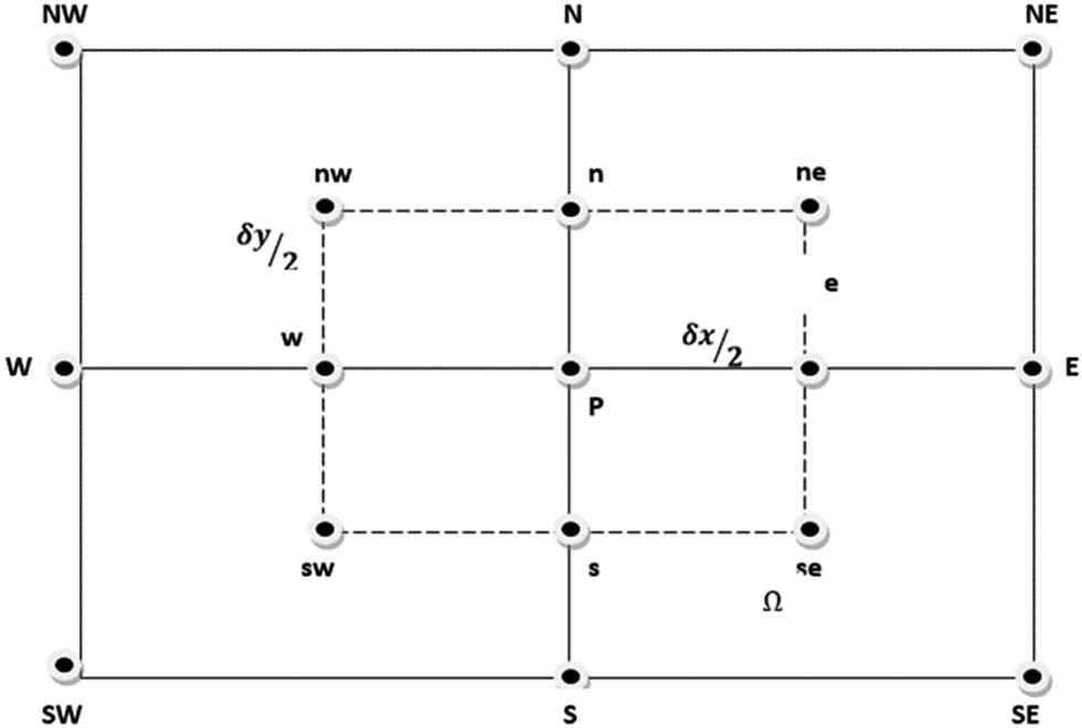
Rectangular-shaped control volume around a grid point P.
The mathematical expressions for the FVM are given below:
Or
As the domain
Here the relations mentioned above take the form
One by one the evaluation of integrals yields the following expressions:
The mathematical expression for the second term is given below:
Moreover,
At the end, we obtain
This method is a widely employed numerical technique for solving PDEs arising in various fields of science and engineering. It is particularly well-suited for problems involving the conservation of physical quantities, such as mass, energy, or momentum. The FVM offers several advantages, including its ability to handle complex geometries and its inherent conservation properties.
For the case when no obstruction is present in the cavity, we compare our numerical results (in Table 1) with those presented by Ali et al. [28] based on the spectral method and a finite difference scheme over a stretched grid.
Comparison of our numerical results with the literature in the absence of any obstruction for
| f Re | Nu | |||||
|---|---|---|---|---|---|---|
| Grid | Finite difference method Ali et al. [28] | Spectral method Ali et al. [28] | FVM (present study) | FDM Ali et al. [28] | Spectral method Ali et al. [28] | FVM (present study) |
|
|
862.5459 | 863.1074 | 863.0055 | 37.9579 | 37.8454 | 37.8251 |
|
|
863.5687 | 863.8322 | 863.2211 | 37.9283 | 37.8977 | 37.8734 |
|
|
863.7380 | 863.9398 | 863.3166 | 37.9234 | 37.9088 | 37.8910 |
|
|
863.9108 | 864.0353 | 863.9985 | 37.9183 | 37.9107 | 37.9087 |
|
|
863.9833 | 864.0735 | 864.0214 | 37.9162 | 37.9113 | 37.9095 |
Table 2 provides the analysis of numerical uncertainty analysis in the study.
Numerical solution for W (x, y) along the line y = 0.2 for different step-sizes
|
|
|||||||
|---|---|---|---|---|---|---|---|
| x |
|
|
Uncertainty |
|
Uncertainty |
|
Uncertainty |
| 0 | 0 | 0 | 0 | 0 | 0 | 0 | 0 |
| 0.1 | 4.8965 | 4.9437 | 0.0472 | 4.9632 | 0.0195 | 4.9719 | 0.0087 |
| 0.2 | 7.0253 | 7.1353 | 0.1100 | 7.1823 | 0.0470 | 7.2038 | 0.0215 |
| 0.3 | 7.5583 | 7.7474 | 0.1891 | 7.8303 | 0.0829 | 7.8688 | 0.0385 |
| 0.4 | 7.4196 | 7.6558 | 0.2362 | 7.7622 | 0.1064 | 7.8124 | 0.0502 |
| 0.5 | 7.3650 | 7.5707 | 0.2057 | 7.6658 | 0.0951 | 7.7113 | 0.0455 |
| 0.6 | 7.6255 | 7.7479 | 0.1224 | 7.8057 | 0.0578 | 7.8335 | 0.0278 |
| 0.7 | 7.8206 | 7.8647 | 0.0441 | 7.8857 | 0.0210 | 7.8957 | 0.0100 |
| 0.8 | 7.2065 | 7.2171 | 0.0106 | 7.2211 | 0.0040 | 7.2227 | 0.0016 |
| 0.9 | 4.9777 | 4.9805 | 0.0028 | 4.9807 | 0.0002 | 4.9804 | 0.0003 |
| 1.0 | 0 | 0 | 0 | 0 | 0 | 0 | 0 |
4 Results and discussion
This section is devoted to study the impact of the governing parameters not only on the velocity and temperature fields but also on the product of the fanning factor f, Nusselt number Nu, and the Reynolds number Re, which are given below:
The thermos-physical properties of nanofluid are mentioned in Tables 3 and 4.
Fixed values of copper and water
| Nanofluid properties | Copper (Cu) | H2O |
|---|---|---|
|
|
8,933 | 997 |
|
|
385 | 4,180 |
|
|
400 | 0.6071 |
Physical properties of nanofluid
| Nanofluid properties | Mathematical formula |
|---|---|
| Heat capacitance
|
|
| Dynamic viscosity (
|
|
| Thermal conductivity
|
|
| Density
|
|
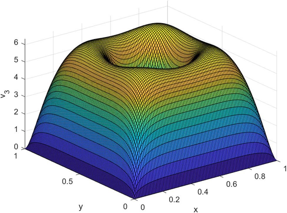
Figures 3–9 show that the pressure gradient causes a significant rise in the flow velocity. The relationship between pressure gradients and flow velocity is a fundamental principle in fluid dynamics that is both fascinating and practical. When we talk about a pressure gradient, we are essentially describing how pressure changes within a fluid system. As the fluid moves from an area of higher pressure to an area of lower pressure, it is essentially responding to this pressure difference. Due to this phenomenon, there is an increase in the flow velocity. This is due to the conservation of energy principle and controlled by the Bernoulli’s equation, i.e., as liquid passes from high pressure region to low-pressure region, its kinetic energy increases. practical applications. In many practical cases, this relationship is crucial. For example, aircrafts use pressure gradients in this way to generate lift: by increasing the flow velocity over the curved upper surface of a wing.

Velocity distribution for

Velocity distribution for

Velocity distribution for

Velocity distribution for
Velocity distribution for

Velocity distribution for

Change in velocity in the middle of the duct with the pressure gradient.
A remarkable rise in the dimensionless temperature is noted with the pressure gradient (Figures 10–16). The interaction between pressure gradients and flow temperature provides the link to other domains where fluid flows are encountered. When a fluid undergoes a transition in its thermodynamics due to change in pressure along its path, this pressure increase in the fluid causes an increased energy density within the fluid. This increased energy level results an increase in the temperature, a phenomenon that is explained by adiabatic heating. But in simple terms, the molecules contained inside a fluid interact more strongly with each other as it is forced through an area of higher pressure, and these interactions lead to a gain in energy known as kinetic energy – or heat. This has major consequences for applications in industrial processes up to geophysical phenomena.

Temperature distribution for

Temperature distribution for

Temperature distribution for

Temperature distribution for

Temperature distribution for

Temperature distribution for

Change in temperature in the middle of the duct with the pressure gradient.
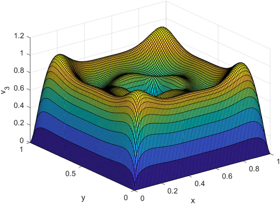
Now, from Figures 17–22, it is seen that the external magnetic field decelerates the flow in the present geometry. Relations between pressure gradients and flow temperature in free-standing fluids are fundamental to fluid dynamics of wide scope. Within the range of a fluid, changing pressure as it flows over a perfect level surface and there is no statement that how this change occurs or what its thermodynamic qualities are alluded to as compressible streams. The greater the pressure, the higher the energy contained in the fluid. This high energy state results in a temperature rise, which describes adiabatic heating. In simplest form, fluid molecules are urged through the higher-pressure area, those interactions accelerate their rate of energy exchange (aka kinetic energy) meaning they will then show an increased temperature. Such an effect has important impacts in applications from industrial processes to geophysical phenomena.

Velocity distribution for

Velocity distribution for

Velocity distribution for

Velocity distribution for

Velocity distribution for

Change in velocity in the middle of the duct with the magnetic field intensity.
Figures 23–28 show that the external magnetic field decelerates the flow in the present geometry. From a physical point of view, when a fluid medium is exposed to an external magnetic field, it initiates a cascade of effects that lead to alterations in thermal behavior. This arises from the magneto-thermodynamic properties inherent to the fluid. The presence of a magnetic field influences the motion and energy states of the fluid’s constituent particles, which in turn impacts their kinetic behavior. As a consequence, the fluid experiences a reduction in temperature, a phenomenon referred to as magnetocaloric cooling.

Temperature distribution for

Temperature distribution for

Temperature distribution for

Temperature distribution for

Temperature distribution for

Change in temperature in the middle of the duct with the magnetic field intensity.
Tables 5–7 describe the results for the numerical data of the problem. The impact of the main problem parameters on the shear stress f Re and the Nusselt number Nu can be examined from these Tables.
Variation in f
Re and Nu with M and Ra, for the fixed
| f Re | Nu | |||||
|---|---|---|---|---|---|---|
| M | Ra = 1,000 | Ra = 10,000 | Ra = 50,000 | Ra = 1,000 | Ra = 10,000 | Ra = 50,000 |
| 0 | 0.2666 | 0.7492 | 2.5003 | 40.2846 | 44.9223 | 59.0917 |
| 10 | 0.6580 | 1.1197 | 2.8627 | 42.8179 | 46.3360 | 58.3918 |
| 20 | 1.7732 | 2.2042 | 3.9264 | 46.6720 | 48.8617 | 57.3482 |
| 30 | 3.5616 | 3.9708 | 5.6673 | 49.6202 | 51.0300 | 56.8467 |
| 40 | 6.0112 | 6.4057 | 8.0778 | 51.7104 | 52.6764 | 56.7874 |
| 50 | 9.1194 | 9.5038 | 11.1548 | 53.2228 | 53.9209 | 56.9427 |
Variation in f
Re and Nu with M and
| f Re | Nu | |||||
|---|---|---|---|---|---|---|
|
|
M = 0 | M = 10 | M = 20 | M = 0 | M = 10 | M = 20 |
| 0 | 2.0122 | 2.4684 | 3.8204 | 51.7777 | 51.9860 | 52.6572 |
| 0.05 | 1.2353 | 1.5955 | 2.6617 | 56.9036 | 57.6244 | 59.1979 |
| 0.10 | 0.8562 | 1.1733 | 2.1082 | 62.6713 | 64.0042 | 66.5844 |
| 0.15 | 0.6397 | 0.9359 | 1.8046 | 69.2449 | 71.2689 | 74.9400 |
| 0.20 | 0.5056 | 0.7926 | 1.6299 | 76.8088 | 79.5824 | 84.4152 |
Variation in f
Re and Nu with
| f Re | Nu | |||||
|---|---|---|---|---|---|---|
|
|
Ra = 1,000 | Ra = 10,000 | Ra = 20,000 | Ra = 1,000 | Ra = 10,000 | Ra = 20,000 |
| 0 | 0.8695 | 1.6649 | 2.4684 | 42.9275 | 47.5622 | 51.9860 |
| 0.05 | 0.6580 | 1.1197 | 1.5955 | 49.5482 | 53.6193 | 57.6244 |
| 0.10 | 0.5594 | 0.8592 | 1.1733 | 56.8934 | 60.4345 | 64.0042 |
| 0.15 | 0.5087 | 0.7159 | 0.9359 | 65.0810 | 68.1319 | 71.2689 |
| 0.20 | 0.4837 | 0.6327 | 0.7926 | 74.2587 | 76.8620 | 79.5824 |
The impact of the Rayleigh number on the flow is to cause a remarkable reduction in the flow velocity (Figures 29–33). In fluid dynamics, the Rayleigh number serves as a critical dimensionless parameter that plays a pivotal role in dictating the behavior of fluid flows. Essentially, it acts as a barometer of the relative significance of buoyancy forces in comparison to viscous forces within a fluid medium. A higher Rayleigh number signifies a scenario where buoyancy forces take precedence, potentially instigating convective motion. Conversely, a lower Rayleigh number indicates a situation where viscous forces dominate, resulting in a more ordered and laminar flow. Hence, as the Rayleigh number increases, it indicates an environment where buoyancy forces are exerting greater influence compared to viscous forces. Consequently, the flow velocity tends to decrease, as the fluid is more prone to convective motion (Figure 34). From Figures 35–40, it is noted that the Rayleigh number increases the flow temperature. However, the impact of the parameter is not very pronounced. From a physical point of view, the increased convective motion (due to the high Rayleigh number) causes regions of differing temperatures to mix more vigorously, resulting in an overall rise in temperature. In simpler terms, an increase in the Rayleigh number intensifies the heat transfer process within the fluid, leading to an elevation in flow temperature.

Velocity distribution for

Velocity distribution for

Velocity distribution for
Velocity distribution for

Velocity distribution for

Velocity change in the middle of the duct with the Rayleigh number.

Thermal distribution for

Thermal distribution for

Thermal distribution for

Thermal distribution for

Thermal distribution for
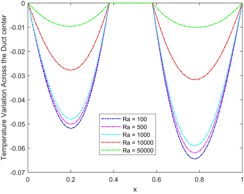
Temperature change in the middle of the duct with the Rayleigh number.
Figure 41 shows that the Nusselt number increases with both the magnetic parameter and the Rayleigh number. In the realm of heat transfer, the Nusselt number stands as a critical dimensionless parameter that plays a pivotal role in characterizing convective heat transfer processes. It quantifies the enhancement of heat transfer due to convection over that of pure conduction. The Nusselt number is paramount and positively-associated with both the magnetic parameter and the Rayleigh number. The convection heat transfer process is highly dependent on the magneto parameter. Increase in the magnetic parameter leads to an increase in the fluid accelerations force and hence high convective heat transfer is obtained. Similarly, the Rayleigh number (a non-dimensional number) describes the importance of buoyancy forces for the viscous flows and, it affects the Nusselt number directly inside the vertical duct. A higher Rayleigh number induces a more vigorous convective flow inside the fluid yielding better heat transfer process.

Nusselt number variation with the magnetic field intensity and the Rayleigh number.
Therefore, it can be deduced that both an elevated magnetic parameter and Rayleigh number contribute to an increase in the Nusselt number, indicating a more pronounced enhancement of heat transfer due to convection.
It is obvious from Figure 42 that the product of the fanning factor and the Reynolds number increases with both the magnetic parameter and the Rayleigh number. The relationship between the fanning factor and the Reynolds number is a crucial aspect to the present problem. It has been observed that the product of these two parameters exhibits a notable increase with variations in both the magnetic parameter and the Rayleigh number. This phenomenon underscores the significant influence of magnetic fields and thermal buoyancy on the flow characteristics of the system under investigation. The concurrent influence of these factors highlights the intricate interplay between magnetic effects and thermal gradients. Figure 43 shows that the product of the fanning factor and the Reynolds number decreases with both pressure gradients. This observation underscores the significant influence of pressure differentials on the flow characteristics. A heightened pressure gradient exerts a notable effect on the flow regime, influencing factors such as flow velocity and boundary layer development. Consequently, this alteration in pressure conditions manifests itself in the product of the fanning factor and the Reynolds number, leading to a reduction in its magnitude (Figure 44). The Nusselt number first increases and then decreases with the nanoparticle volume fraction with an optimum for a 10% concentration of the solid particles (Figure 45) whereas f Re is noted to be always decreasing with the increase in the nanostructure in the fluid (Figure 46).

f Re variation with the magnetic field intensity and the Rayleigh number.

f Re variation with the magnetic field intensity and pressure gradient.
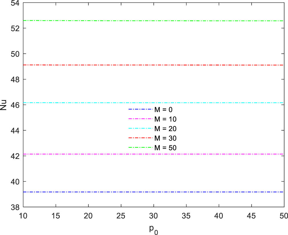
Nusselt number variation with the magnetic field intensity and pressure gradient.

Nusselt number variation with the nanoparticle concentration and the Rayleigh number.

f Re variation with the nanoparticle concentration and the pressure gradient.
5 Conclusion
The purpose of the study is to present the numerical study of external magnetic field effects on the developed laminar flow and thermal characteristics of nanofluid within a vertical square duct containing an obstacle in the middle of the duct, by employing a finite volume approach. We have noted that
A 20% nanoparticle volume fraction resulted in up to 62% rise in the Nusselt number while causing an almost 50% decrease in the factor f Re.
The pressure gradient causes a significant rise in the flow velocity and temperature distribution.
When a flow encounters a magnetic field, the magnetic forces exerted on its charged particles can induce changes in the flow behavior; consequently, the Lorentz force comes into play which acts perpendicular to both the direction of the magnetic field and the fluid flow, leading to a resistance against the flow motion.
Due to the presence of the external magnetic field, the fluid experiences a reduction in temperature, a phenomenon referred to as magnetocaloric cooling.
When the buoyancy forces are exerting greater influence compared to viscous forces, the flow velocity tends to decrease, as the fluid is more prone to convective motion.
An increase in the Rayleigh number intensifies the heat transfer process within the fluid, leading to an elevation in flow temperature.
As the magnetic parameter increases, it enhances the magnetic forces acting on the fluid, consequently intensifying the convective heat transfer.
An increase in the Rayleigh number leads to heightened convective motion within the fluid, resulting in a more efficient heat transfer process. Therefore, it can be deduced that both an elevated magnetic parameter and Rayleigh number contribute to an increase in the Nusselt number, indicating a more pronounced enhancement of heat transfer due to convection.
The Nusselt number first increases and then decreases with the nanoparticle volume fraction with an optimum for a 10% concentration of the solid particles whereas f Re is noted to be always decreasing with the increase in the nanostructure in the fluid.
Acknowledgments
The authors extend their appreciation to the Deanship of Research and Graduate Studies at King Khalid University for funding this work through Large Research Project under grant number RGP2/354/45.
-
Funding information: The authors extend their appreciation to the Deanship of Research and Graduate Studies at King Khalid University for funding this work through Large Research Project under grant number RGP2/354/45.
-
Author contributions: All authors have accepted responsibility for the entire content of this manuscript and approved its submission.
-
Conflict of interest: The authors state no conflict of interest.
References
[1] Ali K, Jamshed W, Suriya Uma Devi S, Ibrahim RW, Ahmad S, Tag El Din ESM. A study of pressure-driven flow in a vertical duct near two current-carrying wires using finite volume technique. Sci Rep. 2022;12:21273. 10.1038/s41598-022-25756-4.Search in Google Scholar
[2] Ortloff CR. Supercritical Froude number flow through ducts with statistically roughened walls. Water. 2023;15:2849. 10.3390/w15152849.Search in Google Scholar
[3] Dolon SN, Hasan MS, Lorenzini G, Mondal RN. A computational modeling on transient heat and fluid flow through a curved duct of large aspect ratio with centrifugal instability. Eur Phys J Plus. 2021;136:382. 10.1140/epjp/s13360-021-01331-0.Search in Google Scholar
[4] Su CC, Lin RH. Experimental studies on flow in convergent and divergent ducts of rectangular cross section. Int J Energy Res. 1997;21(1):77–86.10.1002/(SICI)1099-114X(199701)21:1<77::AID-ER257>3.0.CO;2-GSearch in Google Scholar
[5] Riaz A, Ahammad NA, Alqarni MM, Hejazi HA, Tag-ElDin EM. Peristaltic flow of a viscous fluid in a curved duct with a rectangular cross section. Front Phys. 2022;10:961201. 10.3389/fphy.2022.961201.Search in Google Scholar
[6] Garud KS, Kudriavskyi Y, Lee MS, Kang EH, Lee MY. Numerical study on thermal and flow characteristics of divergent duct with different rib shapes for electric-vehicle cooling system. Symmetry. 2022;14:1696. 10.3390/sym14081696.Search in Google Scholar
[7] Tokgoz N, Sahin B. Experimental studies of flow characteristics in corrugated ducts. Int Commun Heat Mass Transf. 2019;104:41–50. 10.1016/j.icheatmasstransfer.2019.03.003.Search in Google Scholar
[8] Sutevski D, Smolentsev S, Morley N, Abdou M. 3D numerical study of MHD flow in a rectangular duct with a flow channel insert. Fusion Sci Technol. 2011;60(2):513–7. 10.13182/FST11-A12433.Search in Google Scholar
[9] Krasnov D, Zikanov O, Boeck T. Numerical study of magnetohydrodynamic duct flow at high Reynolds and Hartmann numbers. J Fluid Mech. 2012;704:421–46. 10.1017/jfm.2012.256.Search in Google Scholar
[10] Ting HH, Hou SS. Numerical Study of laminar flow and convective heat transfer utilizing nanofluids in equilateral triangular ducts with constant heat flux. Materials. 2016;9:576. 10.3390/ma9070576.Search in Google Scholar
[11] Fonseca WDS, Araujo RCF, Silva MDOE, Cruz DODA. Analysis of the magnetohydrodynamic behavior of the fully developed flow of conducting fluid. Energies. 2021;14:2463. 10.3390/en14092463.Search in Google Scholar
[12] Borrelli A, Giantesio G, Patria MC. Exact solutions in MHD natural convection of a Bingham fluid: fully developed flow in a vertical channel. J Therm Anal Calorim. 2022;147:5825–38. 10.1007/s10973-021-10882-4.Search in Google Scholar
[13] Saleh H, Hashim I. Flow reversal of fully-developed mixed MHD convection in vertical channels. Chin Phys Lett. 2010;27(2):024401. 10.1088/0256-307X/27/2/024401.Search in Google Scholar
[14] Jha BK, Malgwi PB, Aina B. Fully developed magnetohydrodynamics natural convection flow in a vertical micro-porous-channel with Hall effects. Proc Inst Mech Eng, Part N: J Nanomater, Nanoeng Nanosyst. 2019;233(2–4): 73–85. 10.1177/2397791419863596.Search in Google Scholar
[15] Ghosh S, Bég O, Aziz A. A mathematical model for magnetohydrodynamic convection flow in a rotating horizontal channel with inclined magnetic field, magnetic induction and Hall current effects. World J Mech. 2011;1(3):137–54. 10.4236/wjm.2011.13019.Search in Google Scholar
[16] Singh JK, Seth GS, Hussain SM. Thermal performance of hydromagnetic nanofluid flow within an asymmetric channel with arbitrarily conductive walls filled with Darcy-Brinkmann porous medium. J Magn Magn Mater. 2023;582:171034. 10.1016/j.jmmm.2023.171034.Search in Google Scholar
[17] Hussain SM. Irreversibility analysis of time-dependent magnetically driven flow of Sutterby hybrid nanofluid: a thermal mathematical model. Waves Random Complex Media. 2022;1–33. 10.1080/17455030.2022.2089369.Search in Google Scholar
[18] Sajid T, Algarni S, Ahmad H, Alqahtani T, Jamshed W, Eid MR, et al. Exploration of irreversibility process and thermal energy of a tetra hybrid radiative binary nanofluid focusing on solar implementations. Nanotechnol Rev. 2024;13:20240040.10.1515/ntrev-2024-0040Search in Google Scholar
[19] Sankari MS, Rao ME, Shams ZE, Algarni S, Nadeem Sharif M, Alqahtani T, et al. Williamson MHD nanofluid flow via a porous exponentially stretching sheet with bioconvective fluxes. Case Stud Therm Eng. 2024;59:104453.10.1016/j.csite.2024.104453Search in Google Scholar
[20] Nazir U, Sohail M, Singh A, Muhsen S, Galal AM, Tag El Din ESM. Finite element analysis for thermal enhancement in power law hybrid nanofluid. Front Phys. 2022;10:996174. 10.3389/fphy.2022.996174.Search in Google Scholar
[21] Halder A, Bhattacharya A, Biswas N, Manna NK, Mandal DK. Convective heat transport and entropy generation in butterfly-shaped magneto-nanofluidic systems with bottom heating and top cooling. Int J Numer Methods Heat Fluid Flow. 2024;34:837–77. 10.1108/HFF-06-2023-0353.Search in Google Scholar
[22] Manna NK, Saha A, Biswas N, Ghosh K. Effects of enclosure shape on MHD nanofluid flow and irreversibility in different shaped systems under fluid volume constraint. Int J Numer Methods Heat Fluid Flow. 2024;34:666–708. 10.1108/HFF-06-2023-0348.Search in Google Scholar
[23] Biswas N, Mandal DK, Manna NK, Gorla RSR, Chamkha AJ. Hybridized nanofluidic convection in umbrella-shaped porous thermal systems with identical heating and cooling surfaces. Int J Numer Methods Heat Fluid Flow. 2023;33:3164–201. 10.1108/HFF-11-2022-0639.Search in Google Scholar
[24] Chatterjee D, Biswas N, Manna NK, Mandal DK, Chamkha AJ. Magneto-nanofluid flow in cylinder-embedded discretely heated-cooled annular thermal systems: Conjugate heat transfer and thermodynamic irreversibility. J Magn Magn Mater. 2023;569:170442. 10.1016/j.jmmm.2023.170442.Search in Google Scholar
[25] Chatterjee D, Biswas N, Manna NK, Sarkar S. Effect of discrete heating-cooling on magneto-thermal-hybrid nanofluidic convection in cylindrical system. Int J Mech Sci. 2023;238:107852. 10.1016/j.ijmecsci.2022.107852.Search in Google Scholar
[26] Li S, Leng Y, Ali K, Ahmad S, Jamshed W, Saddam EN. Machine learning based evaluation of thermal signature and slip flow dynamics in a lubricated vertical duct exposed to solar energy-induced heating. Int Commun Heat Mass Transf. 2024;152:107308.10.1016/j.icheatmasstransfer.2024.107308Search in Google Scholar
[27] Leng Y, Li S, Al Mesfer MK, Danish M, Ali K, Ahmad S, et al. A finite volume and machine learning based investigation of flow dynamics in a vertical duct heated by the sunlight. Int Commun Heat Mass Transf. 2024;153:107340.10.1016/j.icheatmasstransfer.2024.107340Search in Google Scholar
[28] Ali K, Ahmad S, Ahmad S, Ashraf M, Asif M. On the interaction between the external magnetic field and nanofluid inside a vertical square duct. AIP Adv. 2015;5:107120. 10.1063/1.4934484.Search in Google Scholar
© 2024 the author(s), published by De Gruyter
This work is licensed under the Creative Commons Attribution 4.0 International License.
Articles in the same Issue
- Regular Articles
- Numerical study of flow and heat transfer in the channel of panel-type radiator with semi-detached inclined trapezoidal wing vortex generators
- Homogeneous–heterogeneous reactions in the colloidal investigation of Casson fluid
- High-speed mid-infrared Mach–Zehnder electro-optical modulators in lithium niobate thin film on sapphire
- Numerical analysis of dengue transmission model using Caputo–Fabrizio fractional derivative
- Mononuclear nanofluids undergoing convective heating across a stretching sheet and undergoing MHD flow in three dimensions: Potential industrial applications
- Heat transfer characteristics of cobalt ferrite nanoparticles scattered in sodium alginate-based non-Newtonian nanofluid over a stretching/shrinking horizontal plane surface
- The electrically conducting water-based nanofluid flow containing titanium and aluminum alloys over a rotating disk surface with nonlinear thermal radiation: A numerical analysis
- Growth, characterization, and anti-bacterial activity of l-methionine supplemented with sulphamic acid single crystals
- A numerical analysis of the blood-based Casson hybrid nanofluid flow past a convectively heated surface embedded in a porous medium
- Optoelectronic–thermomagnetic effect of a microelongated non-local rotating semiconductor heated by pulsed laser with varying thermal conductivity
- Thermal proficiency of magnetized and radiative cross-ternary hybrid nanofluid flow induced by a vertical cylinder
- Enhanced heat transfer and fluid motion in 3D nanofluid with anisotropic slip and magnetic field
- Numerical analysis of thermophoretic particle deposition on 3D Casson nanofluid: Artificial neural networks-based Levenberg–Marquardt algorithm
- Analyzing fuzzy fractional Degasperis–Procesi and Camassa–Holm equations with the Atangana–Baleanu operator
- Bayesian estimation of equipment reliability with normal-type life distribution based on multiple batch tests
- Chaotic control problem of BEC system based on Hartree–Fock mean field theory
- Optimized framework numerical solution for swirling hybrid nanofluid flow with silver/gold nanoparticles on a stretching cylinder with heat source/sink and reactive agents
- Stability analysis and numerical results for some schemes discretising 2D nonconstant coefficient advection–diffusion equations
- Convective flow of a magnetohydrodynamic second-grade fluid past a stretching surface with Cattaneo–Christov heat and mass flux model
- Analysis of the heat transfer enhancement in water-based micropolar hybrid nanofluid flow over a vertical flat surface
- Microscopic seepage simulation of gas and water in shale pores and slits based on VOF
- Model of conversion of flow from confined to unconfined aquifers with stochastic approach
- Study of fractional variable-order lymphatic filariasis infection model
- Soliton, quasi-soliton, and their interaction solutions of a nonlinear (2 + 1)-dimensional ZK–mZK–BBM equation for gravity waves
- Application of conserved quantities using the formal Lagrangian of a nonlinear integro partial differential equation through optimal system of one-dimensional subalgebras in physics and engineering
- Nonlinear fractional-order differential equations: New closed-form traveling-wave solutions
- Sixth-kind Chebyshev polynomials technique to numerically treat the dissipative viscoelastic fluid flow in the rheology of Cattaneo–Christov model
- Some transforms, Riemann–Liouville fractional operators, and applications of newly extended M–L (p, s, k) function
- Magnetohydrodynamic water-based hybrid nanofluid flow comprising diamond and copper nanoparticles on a stretching sheet with slips constraints
- Super-resolution reconstruction method of the optical synthetic aperture image using generative adversarial network
- A two-stage framework for predicting the remaining useful life of bearings
- Influence of variable fluid properties on mixed convective Darcy–Forchheimer flow relation over a surface with Soret and Dufour spectacle
- Inclined surface mixed convection flow of viscous fluid with porous medium and Soret effects
- Exact solutions to vorticity of the fractional nonuniform Poiseuille flows
- In silico modified UV spectrophotometric approaches to resolve overlapped spectra for quality control of rosuvastatin and teneligliptin formulation
- Numerical simulations for fractional Hirota–Satsuma coupled Korteweg–de Vries systems
- Substituent effect on the electronic and optical properties of newly designed pyrrole derivatives using density functional theory
- A comparative analysis of shielding effectiveness in glass and concrete containers
- Numerical analysis of the MHD Williamson nanofluid flow over a nonlinear stretching sheet through a Darcy porous medium: Modeling and simulation
- Analytical and numerical investigation for viscoelastic fluid with heat transfer analysis during rollover-web coating phenomena
- Influence of variable viscosity on existing sheet thickness in the calendering of non-isothermal viscoelastic materials
- Analysis of nonlinear fractional-order Fisher equation using two reliable techniques
- Comparison of plan quality and robustness using VMAT and IMRT for breast cancer
- Radiative nanofluid flow over a slender stretching Riga plate under the impact of exponential heat source/sink
- Numerical investigation of acoustic streaming vortices in cylindrical tube arrays
- Numerical study of blood-based MHD tangent hyperbolic hybrid nanofluid flow over a permeable stretching sheet with variable thermal conductivity and cross-diffusion
- Fractional view analytical analysis of generalized regularized long wave equation
- Dynamic simulation of non-Newtonian boundary layer flow: An enhanced exponential time integrator approach with spatially and temporally variable heat sources
- Inclined magnetized infinite shear rate viscosity of non-Newtonian tetra hybrid nanofluid in stenosed artery with non-uniform heat sink/source
- Estimation of monotone α-quantile of past lifetime function with application
- Numerical simulation for the slip impacts on the radiative nanofluid flow over a stretched surface with nonuniform heat generation and viscous dissipation
- Study of fractional telegraph equation via Shehu homotopy perturbation method
- An investigation into the impact of thermal radiation and chemical reactions on the flow through porous media of a Casson hybrid nanofluid including unstable mixed convection with stretched sheet in the presence of thermophoresis and Brownian motion
- Establishing breather and N-soliton solutions for conformable Klein–Gordon equation
- An electro-optic half subtractor from a silicon-based hybrid surface plasmon polariton waveguide
- CFD analysis of particle shape and Reynolds number on heat transfer characteristics of nanofluid in heated tube
- Abundant exact traveling wave solutions and modulation instability analysis to the generalized Hirota–Satsuma–Ito equation
- A short report on a probability-based interpretation of quantum mechanics
- Study on cavitation and pulsation characteristics of a novel rotor-radial groove hydrodynamic cavitation reactor
- Optimizing heat transport in a permeable cavity with an isothermal solid block: Influence of nanoparticles volume fraction and wall velocity ratio
- Linear instability of the vertical throughflow in a porous layer saturated by a power-law fluid with variable gravity effect
- Thermal analysis of generalized Cattaneo–Christov theories in Burgers nanofluid in the presence of thermo-diffusion effects and variable thermal conductivity
- A new benchmark for camouflaged object detection: RGB-D camouflaged object detection dataset
- Effect of electron temperature and concentration on production of hydroxyl radical and nitric oxide in atmospheric pressure low-temperature helium plasma jet: Swarm analysis and global model investigation
- Double diffusion convection of Maxwell–Cattaneo fluids in a vertical slot
- Thermal analysis of extended surfaces using deep neural networks
- Steady-state thermodynamic process in multilayered heterogeneous cylinder
- Multiresponse optimisation and process capability analysis of chemical vapour jet machining for the acrylonitrile butadiene styrene polymer: Unveiling the morphology
- Modeling monkeypox virus transmission: Stability analysis and comparison of analytical techniques
- Fourier spectral method for the fractional-in-space coupled Whitham–Broer–Kaup equations on unbounded domain
- The chaotic behavior and traveling wave solutions of the conformable extended Korteweg–de-Vries model
- Research on optimization of combustor liner structure based on arc-shaped slot hole
- Construction of M-shaped solitons for a modified regularized long-wave equation via Hirota's bilinear method
- Effectiveness of microwave ablation using two simultaneous antennas for liver malignancy treatment
- Discussion on optical solitons, sensitivity and qualitative analysis to a fractional model of ion sound and Langmuir waves with Atangana Baleanu derivatives
- Reliability of two-dimensional steady magnetized Jeffery fluid over shrinking sheet with chemical effect
- Generalized model of thermoelasticity associated with fractional time-derivative operators and its applications to non-simple elastic materials
- Migration of two rigid spheres translating within an infinite couple stress fluid under the impact of magnetic field
- A comparative investigation of neutron and gamma radiation interaction properties of zircaloy-2 and zircaloy-4 with consideration of mechanical properties
- New optical stochastic solutions for the Schrödinger equation with multiplicative Wiener process/random variable coefficients using two different methods
- Physical aspects of quantile residual lifetime sequence
- Synthesis, structure, I–V characteristics, and optical properties of chromium oxide thin films for optoelectronic applications
- Smart mathematically filtered UV spectroscopic methods for quality assurance of rosuvastatin and valsartan from formulation
- A novel investigation into time-fractional multi-dimensional Navier–Stokes equations within Aboodh transform
- Homotopic dynamic solution of hydrodynamic nonlinear natural convection containing superhydrophobicity and isothermally heated parallel plate with hybrid nanoparticles
- A novel tetra hybrid bio-nanofluid model with stenosed artery
- Propagation of traveling wave solution of the strain wave equation in microcrystalline materials
- Innovative analysis to the time-fractional q-deformed tanh-Gordon equation via modified double Laplace transform method
- A new investigation of the extended Sakovich equation for abundant soliton solution in industrial engineering via two efficient techniques
- New soliton solutions of the conformable time fractional Drinfel'd–Sokolov–Wilson equation based on the complete discriminant system method
- Irradiation of hydrophilic acrylic intraocular lenses by a 365 nm UV lamp
- Inflation and the principle of equivalence
- The use of a supercontinuum light source for the characterization of passive fiber optic components
- Optical solitons to the fractional Kundu–Mukherjee–Naskar equation with time-dependent coefficients
- A promising photocathode for green hydrogen generation from sanitation water without external sacrificing agent: silver-silver oxide/poly(1H-pyrrole) dendritic nanocomposite seeded on poly-1H pyrrole film
- Photon balance in the fiber laser model
- Propagation of optical spatial solitons in nematic liquid crystals with quadruple power law of nonlinearity appears in fluid mechanics
- Theoretical investigation and sensitivity analysis of non-Newtonian fluid during roll coating process by response surface methodology
- Utilizing slip conditions on transport phenomena of heat energy with dust and tiny nanoparticles over a wedge
- Bismuthyl chloride/poly(m-toluidine) nanocomposite seeded on poly-1H pyrrole: Photocathode for green hydrogen generation
- Infrared thermography based fault diagnosis of diesel engines using convolutional neural network and image enhancement
- On some solitary wave solutions of the Estevez--Mansfield--Clarkson equation with conformable fractional derivatives in time
- Impact of permeability and fluid parameters in couple stress media on rotating eccentric spheres
- Review Article
- Transformer-based intelligent fault diagnosis methods of mechanical equipment: A survey
- Special Issue on Predicting pattern alterations in nature - Part II
- A comparative study of Bagley–Torvik equation under nonsingular kernel derivatives using Weeks method
- On the existence and numerical simulation of Cholera epidemic model
- Numerical solutions of generalized Atangana–Baleanu time-fractional FitzHugh–Nagumo equation using cubic B-spline functions
- Dynamic properties of the multimalware attacks in wireless sensor networks: Fractional derivative analysis of wireless sensor networks
- Prediction of COVID-19 spread with models in different patterns: A case study of Russia
- Study of chronic myeloid leukemia with T-cell under fractal-fractional order model
- Accumulation process in the environment for a generalized mass transport system
- Analysis of a generalized proportional fractional stochastic differential equation incorporating Carathéodory's approximation and applications
- Special Issue on Nanomaterial utilization and structural optimization - Part II
- Numerical study on flow and heat transfer performance of a spiral-wound heat exchanger for natural gas
- Study of ultrasonic influence on heat transfer and resistance performance of round tube with twisted belt
- Numerical study on bionic airfoil fins used in printed circuit plate heat exchanger
- Improving heat transfer efficiency via optimization and sensitivity assessment in hybrid nanofluid flow with variable magnetism using the Yamada–Ota model
- Special Issue on Nanofluids: Synthesis, Characterization, and Applications
- Exact solutions of a class of generalized nanofluidic models
- Stability enhancement of Al2O3, ZnO, and TiO2 binary nanofluids for heat transfer applications
- Thermal transport energy performance on tangent hyperbolic hybrid nanofluids and their implementation in concentrated solar aircraft wings
- Studying nonlinear vibration analysis of nanoelectro-mechanical resonators via analytical computational method
- Numerical analysis of non-linear radiative Casson fluids containing CNTs having length and radius over permeable moving plate
- Two-phase numerical simulation of thermal and solutal transport exploration of a non-Newtonian nanomaterial flow past a stretching surface with chemical reaction
- Natural convection and flow patterns of Cu–water nanofluids in hexagonal cavity: A novel thermal case study
- Solitonic solutions and study of nonlinear wave dynamics in a Murnaghan hyperelastic circular pipe
- Comparative study of couple stress fluid flow using OHAM and NIM
- Utilization of OHAM to investigate entropy generation with a temperature-dependent thermal conductivity model in hybrid nanofluid using the radiation phenomenon
- Slip effects on magnetized radiatively hybridized ferrofluid flow with acute magnetic force over shrinking/stretching surface
- Significance of 3D rectangular closed domain filled with charged particles and nanoparticles engaging finite element methodology
- Robustness and dynamical features of fractional difference spacecraft model with Mittag–Leffler stability
- Characterizing magnetohydrodynamic effects on developed nanofluid flow in an obstructed vertical duct under constant pressure gradient
- Study on dynamic and static tensile and puncture-resistant mechanical properties of impregnated STF multi-dimensional structure Kevlar fiber reinforced composites
- Thermosolutal Marangoni convective flow of MHD tangent hyperbolic hybrid nanofluids with elastic deformation and heat source
- Investigation of convective heat transport in a Carreau hybrid nanofluid between two stretchable rotatory disks
- Single-channel cooling system design by using perforated porous insert and modeling with POD for double conductive panel
- Special Issue on Fundamental Physics from Atoms to Cosmos - Part I
- Pulsed excitation of a quantum oscillator: A model accounting for damping
- Review of recent analytical advances in the spectroscopy of hydrogenic lines in plasmas
- Heavy mesons mass spectroscopy under a spin-dependent Cornell potential within the framework of the spinless Salpeter equation
- Coherent manipulation of bright and dark solitons of reflection and transmission pulses through sodium atomic medium
- Effect of the gravitational field strength on the rate of chemical reactions
- The kinetic relativity theory – hiding in plain sight
- Special Issue on Advanced Energy Materials - Part III
- Eco-friendly graphitic carbon nitride–poly(1H pyrrole) nanocomposite: A photocathode for green hydrogen production, paving the way for commercial applications