Numerical simulation for the slip impacts on the radiative nanofluid flow over a stretched surface with nonuniform heat generation and viscous dissipation

Ahmed Alkaoud; Mohamed M. Khader; Ali Eid; Ahmed M. Megahed

doi:10.1515/phys-2024-0028

Article Open Access

Numerical simulation for the slip impacts on the radiative nanofluid flow over a stretched surface with nonuniform heat generation and viscous dissipation

Ahmed Alkaoud , Mohamed M. Khader , Ali Eid and Ahmed M. Megahed

Published/Copyright: June 4, 2024

Published by

Become an author with De Gruyter Brill

Submit Manuscript Author Information Explore this Subject

From the journal Open Physics Volume 22 Issue 1

Abstract

The growing fascination with nanofluid flow is motivated by its potential applications in a variety of industries. Therefore, the objective of this research article is to conduct a numerical simulation of the Darcy porous medium flow of Newtonian nanofluids over a vertically permeable stretched surface, considering magnetohydrodynamic mixed convection. Various attributes, such as the impacts of slip, thermal radiation, viscous dissipation, and nonuniform heat sources, are integrated to explore the behavior of the flow. The utilization of the boundary layer theory helps to describe the physical problem as a system of partial differential equations (PDEs). These derived PDEs are then converted to a system of ordinary differential equations (ODEs) through the application of suitable conversions. The outcomes are obtained using the finite difference method, and the effects of parameters on nanofluid flow are compared and visualized through both tabular and graphical representations. The outcomes have been computed and subjected to a comparative analysis with previously published research, revealing a remarkable degree of agreement and consistency. Consequently, these innovative discoveries in heat transfer could prove beneficial in addressing energy storage challenges within the contemporary technological landscape. The noteworthy main findings indicate that when the porous parameter, magnetic number, velocity slip parameter, viscosity parameter, and Brownian motion parameter are assigned higher values, there is an observable expansion in the temperature field. Due to these discoveries, we can enhance the management of temperature in diverse settings by effectively modulating the heat flow.

Keywords: Newtonian nanofluid; slip impacts; nonuniform heat generation; viscous dissipation; finite difference method

Nomenclature

a: positive value representing the rate of stretching
B 0: the magnitude of a magnetic field
C: the concentration of nanoparticles in the base fluid
C w: the fluid concentration adjacent to the sheet
C ∞: fluid concentration away the sheet
Cf x: the coefficient that quantifies friction on a surface
D B: coefficient of diffusion
D T: coefficient of thermophoresis phenomenon
Ec: dissipation factor (Eckert number)
c p: specific heat
f: dimensionless stream function
Gc: modified Grashof number
Gr: Grashof number
k: the permeability property of the porous medium
k *: absorption coefficient within the medium
Le: Lewis number
L 1 , L 2 , L 3: slip velocity, thermal slip, concentration slip, respectively
M: the parameter of the magnetic field
Nu x: Nusselt number
Pr: dimensionless parameter related to Prandtl
q ‴: the nonuniform heat sink or source
q r: the flux of radiant heat
Re: Reynolds number at a particular point
R: radiation parameter
T: dimension temperature
T ∞: dimension temperature of the nanofluid at a distance from the sheet
u , v: the components of the velocity in the x and y -axis direction, respectively
U w: velocity related to stretching
v 0: suction velocity
x , y: Cartesian coordinates
: Greek symbols
τ: the ratio of heat capacity between the nanomaterial and the fluid
δ 1 , δ 2 , δ 3: slip coefficient for the velocity, temperature, and concentration, respectively
ν: kinematic viscosity
σ: Stefan-Boltzmann constant
ρ: density coefficient
ρ ∞: density coefficient at ambient
β: porous parameter
β c: coefficient of the concentration expansion
β t: coefficient of the thermal expansion
μ: viscosity factor
μ ∞: ambient viscosity factor
κ: thermal conductivity
ε: the suction parameter
γ , γ *: heat generation characteristics
η: dimensionless variable
θ ( η ): dimensionless temperature
Ω b: Brownian motion parameter
Ω t: thermophoresis parameter
α: viscosity parameter
ϕ ( η ): dimensionless nanofluid concentration
ψ: stream function
: Superscripts
′: derivative concerning the nondimensional parameter η
w: condition at the sheet
∞: condition away the sheet

1 Introduction

The examination of the fluid flow obtained from the extension of a stretching surface (SS) holds a prominent and captivating position within the realm of fluid mechanics. This significance is primarily attributed to its relevance and applicability in various domains such as the engineering, business, and applied sciences. In a groundbreaking investigation, Sakiadis [1] delved into the analysis of boundary layer flow (BLF) occurring over a continuously advancing flat surface. Several years later, Crane [2] achieved a significant milestone by discovering a precise solution for the BLF that occurs when a sheet is subjected to stretching. Grubka and Bobba, as described in their research [3], successfully tackled the energy equation using Kummer’s function. Their study illuminated the influence of temperature-related parameters on the distribution of temperature within the system.

To impact the efficiency of heat transfer (HT), the thermal conductivity must be at a high level. In contrast to traditional fluids, metals excel in conducting thermal energy, displaying remarkable efficiency in this regard. Due to their relatively low thermal conductivity, traditional HT fluids like ethylene glycol and water fall short when it comes to fulfilling the requirements of contemporary cooling applications. As implied by its name, nanofluid comprises the base fluid blended with extremely fine nanoparticles [4]. To effectively utilize nanofluids across various practical applications, it is imperative to possess a comprehensive understanding of the fundamental traits exhibited by nanofluids, which encompass properties such as the thermal conductivity, viscosity, and specific heat [5]. Nanofluids find themselves employed in a multitude of beneficial and practical applications, including but not limited to refrigeration, air conditioning, microelectronics, and as coolants for portable computer processors [6–10]. Nanofluids could potentially serve as a valuable antibacterial agent to combat antibiotic resistance, offering a promising alternative to address this pressing issue. Furthermore, the utilization of magnetic nanofluid systems is of paramount importance in the fields of drug delivery and biomedical technology. These systems play a crucial role in diverse applications such as differential diagnosis, hyperthermia treatment, and the precise delivery of therapeutic agents to specific targets within the body [11].

Numerical methods are essential for solving nonlinear systems of equations, which are prevalent in fields like engineering, physics, and economics. Nonlinear systems, unlike linear ones, have equations with nonlinear terms, making analytical solutions challenging. Methods like Newton–Raphson iteratively refine initial guesses, updating estimates based on the system’s local behavior to converge toward actual solutions. Several crucial numerical methods including the Crank–Nicolson time-integration scheme [12], finite differences with Lucas polynomials [13], a hybrid local meshless method [14] and shooting method [15,16] are utilized for solving nonlinear systems. These numerical methods offer effective tools for addressing complex relationships, allowing researchers and practitioners to obtain solutions for problems that lack analytical resolutions. The implicit finite difference method (FDM) [17] is a numerical technique frequently applied in solving ordinary differential equations (ODEs). It determines future values through a system of equations involving both current and future unknowns, enabling simultaneous consideration of time steps. Widely used in computational physics and engineering, this method is valued for its efficiency and accuracy in approximating solutions to time-dependent problems.

In this work, we will use the implicit FDM as a numerical method to solve the problem under study. This method has been incorporated by many papers to solve a wide range of ODEs. Through much research [17–19], this method is a reliable tool for dealing with a wide range of problem types. By using this method, the differential equations that express the model under study can be transformed into a nonlinear system of algebraic equations, and then the Newton iteration method is used to solve this system. Many scientists have noted the ability of the FDM to overcome problems and difficulties that may arise during calculations if other numerical methods are used, such as the finite element method [20]. This technique has been used to obtain numerical solutions to many different problems, including the fractional diffusion equation [21], two-sided space fractional wave equation [22], fractional differential equations arising from optimization problems [23], and physical problem of the unsteady Casson fluid flow with heat flux [24].

A comprehensive review of the existing literature reveals a plethora of scholarly papers dedicated to the investigation of nanofluid flow problems, which have been tackled using a combination of semi-analytical and numerical methodologies. In numerous scholarly articles, it is a common practice to treat the viscosity of nanofluids as a constant parameter, while simultaneously overlooking the effects of slip in terms of velocity, temperature, and concentration within the fluid. While it is feasible to modify the viscosity of nanofluids in engineering processes, it is indeed a viable option. Considering these factors, the innovation and pursuit in our present research revolve around examining the dissipative magnetohydrodynamic (MHD) behavior of nanofluid flow over a porous Darcian medium. This particular flow is initiated by a permeable vertical stretching sheet and is further impacted by nonuniform heat generation and thermal radiation. Our chosen methodology for conducting this investigation is through the application of numerical techniques, with a specific focus on employing the FDM.

2 Flow model formulations

Consider a vertical surface that is being stretched linearly according to the relation U w = a x , where a signifies a positive value representing the rate of stretching. The surface of the sheet is located at y -coordinate equal to zero. On this surface, there is a consistent flow of a viscous Newtonian nanofluid that occurs in two dimensions. This flow is limited to when the y -coordinate is greater than zero (Figure 1).

Figure 1

Physical diagram model.

Apply the magnetic field (MF) with strength B 0 to act on the nanofluid flow in a direction perpendicular to it. The induced MF is disregarded as it is believed to be much less potent compared to the applied MF. Also, it is presumed that the model is placed within a porous medium characterized by its permeability, denoted as k . Let us suppose that T w , C w , T ∞ , and C ∞ stand for the temperature and concentration (T–C) at the surface of the nanofluid, as well as the T–C of the surrounding ambient fluid.

All the properties of nanofluids are assumed to remain unchanging, except for viscosity μ , which is modeled to undergo an exponential transformation in response to temperature variations as follows [25]:

(1) μ = μ ∞ e − α T − T ∞ T w − T ∞ .

Here, μ ∞ stands for a constant viscosity value for the nanofluid, which applies at a distance from the surface of the sheet. The nanofluid is examined for the influences of Brownian motion, as indicated by the Brownian diffusion coefficient represented as D B , and for thermophoresis effects, as indicated by the thermophoresis diffusion coefficient denoted as D T . The flow equations governing the behavior of the viscous nanofluid, taking into account factors like a MF, viscous dissipation, slip conditions, variable thermal viscosity, heat generation, and thermal radiative flow, are expressed within the framework of an approximate boundary layer as [26] ( ∇ = ( ∂ ∂ x , ∂ ∂ y ) ):

(2) ∇ . ( u , v ) = 0 ,

(3) ( u , v ) . ∇ u = 1 ρ ∞ ∂ ∂ y μ ∂ u ∂ y − μ ρ ∞ k u + g [ β c ( C − C ∞ ) + β t ( T − T ∞ ) ] − σ B 0 2 ρ ∞ u ,

(4) ( u , v ) . ∇ T = κ ρ ∞ c p ∂ 2 T ∂ y 2 + 1 ρ ∞ c p q ‴ − ∂ q r ∂ y + τ D B ∂ C ∂ y ∂ T ∂ y + D T T ∞ ∂ T ∂ y 2 + μ ρ ∞ c p ∂ u ∂ y 2 ,

(5) ( u , v ) . ∇ C = D T T ∞ ∂ 2 T ∂ y 2 + D B ∂ 2 C ∂ y 2 .

The relevant boundary conditions (BCs) are as described, and these can be found in the work by Awais et al. [27]:

(6) u − U w = δ 1 μ μ ∞ ∂ u ∂ y , T − T w = δ 2 ∂ T ∂ y , at y = 0 ,

(7) v = − v 0 , C − C w = δ 3 ∂ C ∂ y , at y = 0 ,

(8) u → 0 , T → T ∞ , C → C ∞ , as y → ∞ .

Here, we must mention that in the course of our research, we operate under the assumption that the electrical conductivity of the nanofluid under consideration is of a moderate level. This assumption allows us to neglect the irreversibility associated with MHD-resistant heating in the nanofluid flow. In the aforementioned equations, q r represents the radiative heat flux, which can be expressed as a fourth-order relation with temperature, incorporating σ * and k * . This complex expression can be simplified into a linear form as the introduced by Liu and Megahed [25]. Furthermore, q ‴ represents the nonuniform heat sink or source, which can be given as follows [28]:

(9) q ‴ = κ U w ρ ∞ μ x ( γ ( T − T ∞ ) + γ * ( T w − T ∞ ) e − η ) ,

when γ * > 0 and γ > 0 these parameters denote the heat generation characteristics, representing the internal heat production that elevates the temperature. Conversely, when γ * < 0 and γ < 0 , they correspond to the heat-absorbing attributes, causing the temperature to decrease. To derive a nondimensional ODEs for systems (3)–(5) while incorporating the B.Cs (6)–(8), we give some similarity variables as follows:

(10) η = y a ν ∞ , u = U w f ′ ( η ) , v = − a ν ∞ f ( η ) ,

(11) θ ( η ) = T − T ∞ T w − T ∞ , ϕ ( η ) = C − C ∞ C w − C ∞ .

Here, θ ( η ) , ϕ ( η ) , and f ( η ) are the dimensionless of temperature, concentration, and stream function, respectively. The similarity variables selected earlier adhere to the continuity equation (2), respectively. This relationship is based on the connection between the components ( u , v ) of the velocity vector and the stream function ψ that appear as follows:

(12) u = ∂ ψ ∂ y , v = − ∂ ψ ∂ x .

By applying Eqs (10)–(11) to Eqs (3)–(8), we derive the following results:

(13) ( f ‴ − α f ″ θ ′ ) e − α θ − f ′ 2 + f f ″ − M f ′ + Gr θ + Gc ϕ − β e − α θ f ′ = 0 ,

(14) 1 Pr [ ( 1 + R ) θ ″ + ( γ θ + γ * e − η ) e α θ ] + f θ ′ + E c f ″ 2 e − α θ + Ω b θ ′ ϕ ′ + Ω t θ ′ 2 = 0 ,

(15) ϕ ″ + Ω t Ω b θ ″ + PrLe f ϕ ′ = 0 ,

(16) f = ε , f ′ = 1 + L 1 e − α θ f ″ , θ = 1 + L 2 θ ′ , ϕ = 1 + L 3 ϕ ′ , at η = 0 ,

(17) f ′ → 0 , θ → 0 , ϕ → 0 , as ; η → ∞ .

The parameters included in the system of Eqs (13)–(17) that govern the concentration, velocity, and temperature properties of nanofluids, as shown in the previous equations, can be defined as follows:

(18) ε = v 0 ( a ν ∞ ) 1 2 , Gr = g β t ( T w − T ∞ ) U w a , Gc = g β c ( C w − C ∞ ) U w a , β = ν ∞ a k , M = σ B 0 2 a ρ ∞ ,

(19) L 1 = δ 1 a ν ∞ , L 2 = δ 2 a ν ∞ , L 3 = δ 3 a ν ∞ , R = 16 σ * T ∞ 3 3 κ k * , Ec = U w 2 c p ( T w − T ∞ ) ,

(20) Pr = μ ∞ c p κ , Le = κ ρ ∞ c p D B , Ω b = τ ρ ∞ D B ( C w − C ∞ ) μ ∞ , Ω t = τ ρ ∞ D T ( T w − T ∞ ) μ ∞ T ∞ .

The parameters in Eqs (18)–(20) are defined in the Nomenclature section.

3 Quantities essential to engineering applications

The explanations for engineering parameters like the local Nusselt number Nu x Re x (LNN), local Sherwood number Sh x Re x (LSN), and local skin friction coefficient Cf x 2 Re x 1 2 (LSFC), are as stated as follows:

(21) Cf x 2 Re x 1 2 = − ( e − α θ ( 0 ) f ′ ′ ( 0 ) ) , Nu x Re x = − θ ′ ( 0 ) , Sh x Re x = − ϕ ′ ( 0 ) ,

where Re x = U w x ν ∞ highlights the Reynolds number.

4 Solution procedure using FDM

This section is devoted to applying the FDM to provide the numerical solutions to Eqs (13)–(15), which represent the proposed system under study with the boundary conditions (16)–(17). Previously, through many published works, this method has been tested for its accuracy and efficiency in solving different problems. To enable the use of this method, we will use the transformation f ′ ( η ) = g ( η ) to rewrite the system of Eqs (13)–(17) as follows:

(22) f ′ − g = 0 ,

(23) ( g ″ − α g ′ θ ′ ) e − α θ − g 2 + f g ′ − Mg + Gr θ + Gc ϕ − β e − α θ g = 0 ,

(24) ( 1 + R ) θ ″ + ( γ θ + γ * e − η ) e α θ + P r ( f θ ′ + Ec g ′ 2 e − α θ + Ω b θ ′ ϕ ′ + Ω t θ ′ 2 ) = 0 ,

(25) ϕ ″ + Ω t Ω b θ ″ + PrLe f ϕ ′ = 0 ,

(26) f = ε , g = 1 + L 1 e − α θ g ′ , θ = 1 + L 2 θ ′ , ϕ = 1 + L 3 ϕ ′ , at η = 0 ,

(27) g → 0 , θ → 0 , ϕ → 0 , as η → ∞ .

In the FDM, the domain of the problem is divided into some discrete subintervals across a set of nodes. For this, we use the symbols; Δ η = ℏ > 0 to be the mesh size in the η -direction, Δ η = η ∞ ∕ N , with η j = j ℏ for j = 0 , 1 , … , N . Define f k = f ( η k ) , g k = g ( η k ) , θ k = θ ( η k ) , and ϕ k = ϕ ( η k ) .

Let F k , G k , Θ k , and Φ k denote the numerical values of f , g , θ , and ϕ at the kth node, respectively. We take

(28) f ′ ∣ k ≈ f k + 1 − f k − 1 2 ℏ , g ′ ∣ k ≈ g k + 1 − g k − 1 2 ℏ , θ ′ ∣ k ≈ θ k + 1 − θ k − 1 2 ℏ , ϕ ′ ∣ k ≈ ϕ k + 1 − ϕ k − 1 2 ℏ ,

(29) g ″ ∣ k ≈ g k + 1 − 2 g k + g k − 1 ℏ 2 , θ ″ ∣ k ≈ θ k + 1 − 2 θ k + θ k − 1 ℏ 2 , ϕ ″ ∣ k ≈ ϕ k + 1 − 2 ϕ k + ϕ k − 1 ℏ 2 .

One of the basics of applying the FDM is to express the system being solved in a discretized form, then after that, we replace from (28)–(29) into the models (22)–(27). By neglecting truncation errors, this system of ODEs turns into the following system of nonlinear algebraic equations:

(30) F k + 1 − F k − 1 − 2 ℏ G k = 0 , k = 0 , 1 , … , N ,

(31) [ 4 ( G k + 1 − 2 G k + G k − 1 ) − α ( G k + 1 − G k − 1 ) ( Θ k + 1 − Θ k − 1 ) ] e − α Θ k + 2 ℏ F k ( G k + 1 − G k − 1 ) − 4 ℏ 2 [ G k 2 + M G k − Gr Θ k − Gc Φ k + β e − α Θ k G k ] = 0 ,

(32) 4 ( 1 + R ) ( Θ k + 1 − 2 Θ k + Θ k − 1 ) + 4 ℏ 2 ( γ Θ k + γ * e − η k ) e α Θ k + Pr [ 2 ℏ F k ( Θ k + 1 − Θ k − 1 ) + Ec ( G k + 1 − G k − 1 ) 2 e − α Θ k + Ω b ( Θ k + 1 − Θ k − 1 ) ( Φ k + 1 − Φ k − 1 ) + Ω t ( Θ k + 1 − Θ k − 1 ) 2 ] = 0 ,

(33) 2 ( Φ k + 1 − 2 Φ k + Φ k − 1 ) + 2 Ω t Ω b ( Θ k + 1 − 2 Θ k + Θ k − 1 ) + ℏPrLe F k ( Φ k + 1 − Φ k − 1 ) = 0 .

Also, the boundary conditions are as follows:

(34) F 0 = ε , G 0 = 1 + ℏ − 1 L 1 e − α Θ 0 ( G 1 − G 0 ) , Θ 0 = 1 + ℏ − 1 L 2 ( Θ 1 − Θ 0 ) , Φ 0 = 1 + ℏ − 1 L 3 ( Φ 1 − Φ 0 ) , G N = Θ N = Φ N = 0 .

Now we use the Newton iteration method as one of the most important and efficient numerical methods in solving systems of nonlinear algebraic equations to obtain the approximations F j , G j , Θ j , and Φ j , ( j = 0 , 1 , … , N ). In our calculation, we used a suitable initial solution to solve this system with the help of the Mathematica Package, and Newton iteration method.

5 Model validation

The numerical outcomes presented in both graphical representations and tabular formats have been derived using the FDM as the underlying computational approach. Neglecting the impacts of the parameters α , M , Gr , Gc , β , ε , L 1 , L 2 , Ec , R , γ * , γ , Ω b , and Ω t , we are examining the results related to the LNN, which is represented as − θ ′ ( 0 ) . We are making a comparison between our findings and those reported by Wang [29], as well as the research conducted by Gorla and Sidawi [30]. This comparison is carried out across a range of different values of Prandtl Pr number, and the detailed results can be found in Table 1. Our observation reveals a favorable level of conformity in the comparison for every Prandtl Pr value examined. Consequently, we possess a high level of confidence in the precision and reliability of the current findings.

Table 1

Values of − θ ′ ( 0 ) for various values of Pr with the findings of Wang [29], and Gorla and Sidawi [30] when α = M = Gr = Gc = β = ε = L 1 = L 2 = 0 and Ec = R = γ * = γ = Ω b = Ω t = 0

Pr	Wang [29]	Gorla and Sidawi [30]	Current work
0.07	0.0656	0.0656	0.0655896523
0.20	0.1691	0.1691	0.1690785012
0.70	0.4539	0.5349	0.5348802589
2.00	0.9114	0.9114	0.9113569998
7.00	1.8954	1.8905	1.8904750021
20.00	3.3539	3.3539	3.3538800027
70.00	6.4622	6.4622	6.4621599985

6 Numerical outcomes and discussion

This study examines how nanofluid movement, electromagnetic fields, HT mechanisms, and dynamic conductivity influence temperature, velocity, and concentration boundaries within a fluid flow generated by a vertically SS within a porous medium. The governing equations were solved numerically using the FDM within the MATHEMATICA software, and the results were graphically presented to depict the behavior of the problem. Throughout this research, various physical factors are examined for their impact, encompassing parameters related to porosity, magnetism, viscosity, suction, slip velocity, thermal slip, concentration slip, Grashof number, modified Grashof number, Eckert parameter, thermophoresis index, and Brownian motion coefficient. The study assesses how these factors influence concentration, velocity distribution, and temperature, and presents flowcharts illustrating mass distribution across diverse scenarios. The selection of parameter values for this study considers multiple factors, including the nanofluid’s physical properties, boundary conditions, and findings from prior research documented in the literature. In addition, certain values are deliberately chosen to align with theoretical predictions. Moreover, the intervals for these factors lie within the range of 0.0 ≤ β ≤ 1 , 0.0 ≤ M ≤ 1 , 0.0 ≤ ε ≤ 1 , 0.0 ≤ α ≤ 1 , 0.0 ≤ L 1 ≤ 0.4 , 0.0 ≤ Gr ≤ 0.3 , 0.0 ≤ Gc ≤ 1 , 0.0 ≤ γ ≤ 0.2 , 0.0 ≤ Ec ≤ 0.5 , 0.5 ≤ Ω b ≤ 1.5 , 0.0 ≤ Ω t ≤ 0.8 , 0.0 ≤ L 2 ≤ 0.5 , and 0.0 ≤ L 3 ≤ 0.5 .

Figure 2 provides a visual representation of how varying levels of the porous parameter impact the characteristics of f ′ ( η ) , ϕ ( η ) , and θ ( η ) . This graphical representation illustrates how changes in the porous parameter values affect the behavior of these variables. It can be observed that as the porous parameter is increased, there is a noticeable reduction in fluid velocity and a concurrent decrease in the thickness of the BL. Conversely, a different trend is observed for temperature and concentration. Temperature tends to increase with rising values of the porous parameter, while the effect on the concentration field is less pronounced, resulting in a relatively subtle change. From a physical perspective, when the permeability parameter is elevated, the motion of liquid particles experiences heightened opposition or resistance. Consequently, this leads to a decrease in the velocity of nanofluid flow as the porous parameter increases.

$Figure 2 (a) f ′ ( η ) f^{\prime} \left(\eta ) and θ ( η ) \theta \left(\eta ) for various β \beta (b) ϕ ( η ) \phi \left(\eta ) for various β \beta .$

Figure 2

(a) f ′ ( η ) and θ ( η ) for various β (b) ϕ ( η ) for various β .

Figure 3 offers valuable insights into how ϕ ( η ) , θ ( η ) , and f ′ ( η ) profiles evolve with variations in the magnetic parameter M . As illustrated in Figure 3, when we observe an increase in the value of M , there is a corresponding decrease in the velocity profiles and the momentum thickness. This trend suggests that higher values of M lead to a reduction in flow velocities. Furthermore, the same figure implies that elevated values of the magnetic parameter exhibit an augmenting effect on both ϕ ( η ) and θ ( η ) fields. However, it is important to note that this influence is less pronounced when it comes to the concentration field. In other words, higher magnetic parameter values tend to have a more noticeable impact on temperature compared to their effect on concentration. Physically, this phenomenon arises from the expansion of the Lorentz force, impeding the movement of fluid along the sheet. As a result, this force tends to slow down fluid motion while simultaneously accelerating both fluid concentration and temperature within the BL in the nanofluid flow region.

$Figure 3 (a) f ′ ( η ) f^{\prime} \left(\eta ) and θ ( η ) \theta \left(\eta ) for various M M (b) ϕ ( η ) \phi \left(\eta ) for various M M .$

Figure 3

(a) f ′ ( η ) and θ ( η ) for various M (b) ϕ ( η ) for various M .

Figure 4 displays two-dimensional diagrams depicting the dimensionless suction parameter ε at different values to evaluate its influence on f ′ ( η ) , ϕ ( η ) , and θ ( η ) fields. The findings suggest that varying the values of the dimensionless suction parameter results in a reduction in the concentration, velocity, and temperature profiles, as well as a decrease in the corresponding BL thickness. This clearly highlights the significant effect of ε on the flow pattern of nanofluid within a porous medium. Physically, the decrease in nanofluid concentration is associated with an increase in ε . Elevated suction levels lead to the extraction of more fluid particles from the system of motion for the nanofluid flow, thereby causing an overall reduction in nanofluid concentration.

$Figure 4 (a) f ′ ( η ) f^{\prime} \left(\eta ) and θ ( η ) \theta \left(\eta ) for various ε \varepsilon (b) ϕ ( η ) \phi \left(\eta ) for various ε \varepsilon .$

Figure 4

(a) f ′ ( η ) and θ ( η ) for various ε (b) ϕ ( η ) for various ε .

Figure 5 gives a clear representation of how the f ′ ( η ) , θ ( η ) , and ϕ ( η ) change in response to higher values of the viscosity parameter α across the similarity variable η . A greater influence of α results in a higher degree of heating in the nanofluid. This is attributed to the fact that the effect of α on temperature is contingent upon it. The identical figure demonstrates that there is a marginal improvement in nanofluid concentration as the viscosity parameter increases. In contrast, the opposite trend is observed in the velocity field.

$Figure 5 (a) f ′ ( η ) f^{\prime} \left(\eta ) and θ ( η ) \theta \left(\eta ) for various α \alpha (b) ϕ ( η ) \phi \left(\eta ) for various α \alpha .$

Figure 5

(a) f ′ ( η ) and θ ( η ) for various α (b) ϕ ( η ) for various α .

Figure 6 displays the impact of the slip velocity parameter L 1 on the distributions of θ ( η ) , f ′ ( η ) , and ϕ ( η ) . It visually represents how variations in L 1 affect these distribution profiles. Figure 6 reveals distinct patterns: as L 1 rises, there is an increase in both concentration and temperature. Conversely, there is a contrasting trend observed for both the sheet velocity f ′ ( 0 ) and the nanofluid velocity f ′ ( η ) , where they decrease as the slip velocity parameter increases. From a purely physical perspective, when slippage takes place, the decrease in flow velocity outside the sheet is comparatively less than the reduction in velocity at the surface being propelled. Moreover, the investigation of the velocity slip phenomenon and its influence on heat and mass transfer processes has been explored in prior research by Mandal and Pal [31,32]. By referencing their observations on this phenomenon, we can have confidence in our current findings.

$Figure 6 (a) f ′ ( η ) f^{\prime} \left(\eta ) and θ ( η ) \theta \left(\eta ) for various L 1 {L}_{1} and (b) ϕ ( η ) \phi \left(\eta ) for various L 1 {L}_{1} .$

Figure 6

(a) f ′ ( η ) and θ ( η ) for various L 1 and (b) ϕ ( η ) for various L 1 .

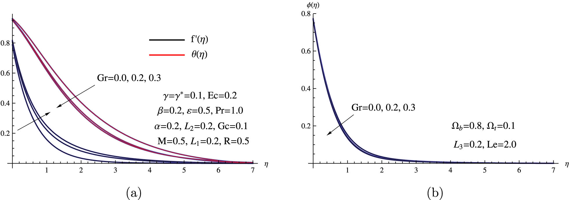
Figure 7 provides a visual representation of how the Grashof number Gr impacts the flow and heat mass characteristics under the condition where all other parameters are held constant. An observation drawn from Figure 7 is that the velocity of the nanofluid within the BL experiences an upsurge when the Grashof number is introduced. In contrast, as the Grashof number escalates, both the temperature and the concentration demonstrate a declining trend. Physically, the increase in nanofluid velocity with an elevation in Gr number can be ascribed to the intensified natural convection spurred by heightened buoyancy forces linked to higher Grashof numbers. Consequently, this results in a more rapid and accelerated fluid motion occurring in the vicinity of the BL.

$Figure 7 (a) f ′ ( η ) f^{\prime} \left(\eta ) and θ ( η ) \theta \left(\eta ) for various Gr and (b) ϕ ( η ) \phi \left(\eta ) for various Gr.$

Figure 7

(a) f ′ ( η ) and θ ( η ) for various Gr and (b) ϕ ( η ) for various Gr.

Figure 8 illustrates how alterations in the modified Grashof number Gc impact the distributions of nanoparticle ϕ ( η ) , f ′ ( η ) , and θ ( η ) in the flow of nanofluid and the associated heat mass transfer. This diagram illustrates that as Gc rises, the velocity of the nanofluid also increases. In practical terms, this escalation in the modified Gc leads to the development of a concentration gradient within the flow, which, in turn, diminishes the BL and amplifies the fluid’s velocity. Similarly, the depicted figure clarifies that the modified Grashof number has an impact on both the concentration and temperature, albeit in contrasting patterns. Physically, as the modified Grashof number rises, buoyancy forces take precedence over viscous forces, leading to increased fluid motion and enhanced convective HT. This intensified buoyancy-driven flow carries away more heat, resulting in a decrease in nanofluid temperature.

$Figure 8 (a) f ′ ( η ) f^{\prime} \left(\eta ) and θ ( η ) \theta \left(\eta ) for various Gc and (b) ϕ ( η ) \phi \left(\eta ) for various Gc.$

Figure 8

(a) f ′ ( η ) and θ ( η ) for various Gc and (b) ϕ ( η ) for various Gc.

Figure 9 depicts how the nanofluid temperature θ ( η ) is affected by variations in γ , γ * , and Ec. The observation made indicates that as both the γ , γ * , and Ec are elevated, there is a corresponding augmentation in the temperature distribution of the nanofluid. In simpler terms, increasing these parameters leads to a higher temperature profile within the nanofluid. Physically, an increase in the heat generation parameter means more heat is produced in the nanofluid, boosting its internal energy and, consequently, raising its temperature. This results in a higher temperature distribution within the nanofluid due to the generated energy. Furthermore, it is understood that the Ec is defined as the ratio of the flow’s kinetic energy (KE) to the enthalpy differences in the BL. In physical terms, this ratio represents the conversion of the KE into internal energy through work done against viscous forces.

$Figure 9 (a) θ ( η ) \theta \left(\eta ) for various γ , γ * \gamma ,{\gamma }^{* } , and (b) θ ( η ) \theta \left(\eta ) for various Ec.$

Figure 9

(a) θ ( η ) for various γ , γ * , and (b) θ ( η ) for various Ec.

Figure 10 illustrates how changes in the Ω b impact the distribution of θ ( η ) and ϕ ( η ) . Raising Ω b significantly increases temperature values across the entire range. Nanoparticles with smaller geometric sizes exhibit greater Brownian motion, which aids thermal diffusion in the BL by enhancing thermal conduction. In contrast, larger nanoparticles have reduced Brownian motion, which hinders thermal conduction. On the contrary, increased Brownian motion parameter values will inhibit the movement of nanoparticles from the surface into the fluid region. This will result in a reduction of nanoparticle concentration values within the boundary layer, as depicted in the corresponding figure. The arrangement of nanoparticles within the stretching sheet domain can be controlled through the Brownian motion mechanism, and cooling of the domain can likewise be attained by using lower Brownian motion parameter values.

$Figure 10 (a) θ ( η ) \theta \left(\eta ) for various Ω b {\Omega }_{b} and (b) ϕ ( η ) \phi \left(\eta ) for various Ω b {\Omega }_{b} .$

Figure 10

(a) θ ( η ) for various Ω b and (b) ϕ ( η ) for various Ω b .

Figure 11 illustrates how changes in the thermophoresis parameter Ω t affect the distribution of θ ( η ) and ϕ ( η ) within the domain. The thicknesses of both the thermal and concentration BLs increase as the Ω t is raised. Thermophoresis plays a dual role in the boundary layer by facilitating the diffusion of both thermal energy and species, such as nanoparticles. Physically, Ω t plays a pivotal role in facilitating the transfer of both temperature and particles within the boundary layer. When the system undergoes heating, a favorable consequence unfolds, wherein there is an improvement in the dispersion of nanoparticles. This refined distribution of nanoparticles is directly linked to the augmentation of the Ω t effect.

$Figure 11 (a) θ ( η ) \theta \left(\eta ) for various Ω t {\Omega }_{t} and (b) ϕ ( η ) \phi \left(\eta ) for various Ω t {\Omega }_{t} .$

Figure 11

(a) θ ( η ) for various Ω t and (b) ϕ ( η ) for various Ω t .

Figure 12(a) illustrates how changes in the thermal slip parameter L 2 impact the distribution of θ ( η ) . As the L 2 decreases, it signifies a scenario where the efficiency of HT between the solid surface and the fluid diminishes. This decline in efficiency, in turn, leads to a notable reduction in the temperature of the nanofluid. This decrease in nanofluid temperature is primarily attributed to the fact that there is less effective thermal conduction occurring across the boundary between the solid surface and the fluid. In simpler terms, a lower L 2 results in less-efficient heat exchange between the solid and the fluid, consequently causing a drop in the nanofluid’s temperature. Figure 12(b) shows how alterations in the concentration slip parameter L 3 affect the ϕ ( η ) of nanofluid. when the L 3 decreases, it means there is less variation in concentration at the solid–fluid interface. This results in a more even and consistent nanofluid concentration along the boundary. Consequently, the nanofluid concentration either remains relatively stable or experiences a slight decrease due to reduced mass transfer processes. In a physical sense, this occurs because an elevation in the concentration slip parameter indicates a reduction in the molecular diffusivity within the flow system. Consequently, there is a decline in the net flux of the species, leading to a substantial decrease in the ϕ ( η ) distribution of the nanofluid.

$Figure 12 (a) θ ( η ) \theta \left(\eta ) for various L 2 {L}_{2} and (b) ϕ ( η ) \phi \left(\eta ) for various L 3 {L}_{3} .$

Figure 12

(a) θ ( η ) for various L 2 and (b) ϕ ( η ) for various L 3 .

Table 2 presents data on the HT rate near the heated surface, represented by the Nusselt number Nu x Re x , the mass transfer rate close to the surface, indicated by the Sherwood number Sh x Re x , and the shear stress rate along the surface, expressed as the skin friction coefficient Cf x 2 Re x 1 2 . These values are provided for various combinations of the governing parameters. The table reveals that as the suction parameter and modified Gc, along with the Grashof number itself, increase, there is a significant rise in both the LNN and LSN. Furthermore, the skin friction coefficient values exhibit a rapid increase when β , M , and ε are raised, while the opposite trend is observed for the α , L 1 , and Gc, where the values of LSFC tend to decrease. On the other hand, the local mass transfer coefficient and shear stress rates experience an uptick as the Brownian diffusion parameter rises, whereas the opposite pattern is observed for the thermophoresis parameter, where these rates tend to decrease.

Table 2

Values of Nu x Re x , Cf x 2 Re x 1 2 , and Sh x Re x for various values of β , M , ε , α , L 1 , Gr, Gc, γ * , γ , Ec, Ω b , and Ω t with Pr = 1.0 , L 2 = L 3 = 0.2 , and Le = 2.0

β	M	ε	α	L 1	Gr	Gc	γ * , γ	Ec	Ω b	Ω t	Cf x 2 Re x 1 2	Nu x Re x	Sh x Re x
0.0	0.5	0.5	0.2	0.2	0.1	0.1	0.1	0.2	0.8	0.1	0.968025	0.226756	1.154150
0.5	0.5	0.5	0.2	0.2	0.1	0.1	0.1	0.2	0.8	0.1	1.064352	0.200846	1.136731
1.0	0.5	0.5	0.2	0.2	0.1	0.1	0.1	0.2	0.8	0.1	1.145847	0.180124	1.122253
0.2	0.0	0.5	0.2	0.2	0.1	0.1	0.1	0.2	0.8	0.1	0.879391	0.250044	1.169843
0.2	0.5	0.5	0.2	0.2	0.1	0.1	0.1	0.2	0.8	0.1	1.008742	0.215626	1.146752
0.2	1.0	0.5	0.2	0.2	0.1	0.1	0.1	0.2	0.8	0.1	1.113744	0.189129	1.128194
0.2	0.5	0.0	0.2	0.2	0.1	0.1	0.1	0.2	0.8	0.1	0.825238	0.063892	0.684554
0.2	0.5	0.5	0.2	0.2	0.1	0.1	0.1	0.2	0.8	0.1	1.008742	0.215626	1.146752
0.2	0.5	1.0	0.2	0.2	0.1	0.1	0.1	0.2	0.8	0.1	1.211126	0.407084	1.570501
0.2	0.5	0.5	0.0	0.2	0.1	0.1	0.1	0.2	0.8	0.1	1.072839	0.240241	1.150892
0.2	0.5	0.5	0.5	0.2	0.1	0.1	0.1	0.2	0.8	0.1	0.916164	0.167837	1.139733
0.2	0.5	0.5	1.0	0.2	0.1	0.1	0.1	0.2	0.8	0.1	0.768869	0.029460	1.129964
0.2	0.5	0.5	0.2	0.0	0.1	0.1	0.1	0.2	0.8	0.1	1.367451	0.217978	1.195710
0.2	0.5	0.5	0.2	0.2	0.1	0.1	0.1	0.2	0.8	0.1	1.008742	0.215626	1.146752
0.2	0.5	0.5	0.2	0.4	0.1	0.1	0.1	0.2	0.8	0.1	0.805785	0.208691	1.115460
0.2	0.5	0.5	0.2	0.2	0.0	0.1	0.1	0.2	0.8	0.1	1.060418	0.190407	1.134161
0.2	0.5	0.5	0.2	0.2	0.2	0.1	0.1	0.2	0.8	0.1	0.960962	0.235287	1.157450
0.2	0.5	0.5	0.2	0.2	0.3	0.1	0.1	0.2	0.8	0.1	0.914855	0.248687	1.166436
0.2	0.5	0.5	0.2	0.2	0.1	0.0	0.1	0.2	0.8	0.1	1.029501	0.210972	1.143291
0.2	0.5	0.5	0.2	0.2	0.1	0.4	0.1	0.2	0.8	0.1	0.947954	0.228542	1.156593
0.2	0.5	0.5	0.2	0.2	0.1	1.0	0.1	0.2	0.8	0.1	0.832106	0.250499	1.174175
0.2	0.5	0.5	0.2	0.2	0.1	0.1	0.0	0.2	0.8	0.1	1.019090	0.350663	1.133192
0.2	0.5	0.5	0.2	0.2	0.1	0.1	0.1	0.2	0.8	0.1	1.008742	0.215626	1.146752
0.2	0.5	0.5	0.2	0.2	0.1	0.1	0.2	0.2	0.8	0.1	0.993631	0.031714	1.165356
0.2	0.5	0.5	0.2	0.2	0.1	0.1	0.1	0.0	0.8	0.1	1.010741	0.258438	1.142671
0.2	0.5	0.5	0.2	0.2	0.1	0.1	0.1	0.2	0.8	0.1	1.008742	0.215626	1.146752
0.2	0.5	0.5	0.2	0.2	0.1	0.1	0.1	0.5	0.8	0.1	1.005763	0.151848	1.152858
0.2	0.5	0.5	0.2	0.2	0.1	0.1	0.1	0.2	0.5	0.1	1.010381	0.252388	1.134721
0.2	0.5	0.5	0.2	0.2	0.1	0.1	0.1	0.2	1.5	0.1	1.004602	0.144123	1.155886
0.2	0.5	0.5	0.2	0.2	0.1	0.1	0.1	0.2	0.8	0.0	1.010475	0.224273	1.157733
0.2	0.5	0.5	0.2	0.2	0.1	0.1	0.1	0.2	0.8	0.8	0.998134	0.160812	1.107932

Remark 1

Just as we mentioned earlier, the FDM is one of the numerical methods with more accuracy and high efficiency. It is also known that the error in each of the approximations of the first and second derivatives, which are defined in Eqs (28)–(29) is of the order o( ℏ 2 ). Therefore, we find that the convergence and stability of the used numerical scheme depend greatly on the size of the mesh step ℏ , i.e., if the value of ℏ decreases, then the value of the error decreases. So ℏ is the parameter that controls the stability of the resulting solutions. This is clear in light of the tabular or graphical results, as well as the comparisons made with a special case of the model under study and using another numerical method (Table 1).

7 Conclusions

The primary aim of this research is to examine the transfer of heat and mass in a situation where radiative and magnetic forces influence the flow of a nanofluid over an extending vertical and permeable surface through a porous medium. This analysis takes into account significant factors like nonuniform heat generation and viscous dissipation. Furthermore, the study delves deeply into the comprehensive assessment of heat and mass transfer efficiency, taking into consideration the cumulative influence of varying viscosity, L 1 , L 2 , and L 3 . The governing equations for the flow, initially expressed as partial derivatives, are reduced to a system of ODEs through the utilization of carefully designed similarity transformations. This system is then tackled numerically by employing the FDM. Several significant discrete findings that emerged while examining the influence of parameters on the flow include:

The Nusselt number shows an upward trend as both the Gr and Gc increase, but conversely, it decreases when M and β are raised.
The skin-friction coefficients exhibit an upward trend when the parameters β , M , and ε are increased, but they decrease when the viscosity parameter, slip velocity parameter, and Grashof number are raised.
Increased values were applied to both the parameters Ω b and Ω t , resulting in a significant elevation of the temperature distribution. Specifically, about the temperature distribution.
The velocity profile of the nanofluid flow decreases as the parameters M , L 1 , β , α , and ε are increased.
An increase in the suction parameter results in a reduction in temperature, concentration, velocity, and BL thickness.

Acknowledgments

This work was supported and funded by the Deanship of Scientific Research at Imam Mohammad Ibn Saud Islamic University (IMSIU) (grant number IMSIU-RG23003).

Funding information: This work was supported and funded by the Deanship of Scientific Research at Imam Mohammad Ibn Saud Islamic University (IMSIU) (grant number IMSIURG23003).
Author contributions: Conceptualization: A.A., M.M.K., and A.E.; methodology: A.A., M.M.K. and A.M.M.; software: M.M.K., A.M.M., and A.E.; validation: A.A., M.M.K., and A.M.M.; formal analysis: M.M.K., A.E., and A.M.M.; investigation: A.A., M.M.K., A.E., and A.M.M.; resources: A.A., M.M.K., and A.E.; data curation: A.A., M.M.K., and A.M.M.; writing–original draft preparation: A.A., M.M.K., A.M.M., and A.E.; writing–review and editing: M.M.K., A.E., and A.M.M.; visualization: A.A., M.M.K., A.M.M., and A.E.; supervision: M.M.K. and A.E.; project administration: A.A., M.M.K., and A.E. All authors have accepted responsibility for the entire content of this manuscript and approved its submission.
Conflict of interest: The authors state no conflict of interest.

References

[1] Sakiadis BC. Boundary-layer behavior on continuous solid surfaces: I. Boundary-layer equations for two-dimensional and axisymmetric flow. AIChE J. 1961;7:26–8. 10.1002/aic.690070108Search in Google Scholar

[2] Crane LJ. Flow past a stretching plate. J Appl Math Phys. 1970;21:645–7. 10.1007/BF01587695Search in Google Scholar

[3] Grubka L, Bobba K. Heat transfer characteristics of a continuous, stretching surface with variable temperature. ASME J. Heat Transfer 1985;107:248–50. 10.1115/1.3247387Search in Google Scholar

[4] Choi SUS. Enhancing thermal conductivity of fluid with nanoparticles, developments, and applications of non-Newtonian flow. ASME FED 1995;231:99–105. Search in Google Scholar

[5] Eastman JA, Choi SUS, Li S, Yu W, Tompson LJ. Anomalously increased effective thermal conductivities of ethylene glycol-based nanofluids containing copper nanoparticles. Appl Phys Lett. 2001;78:718–20. 10.1063/1.1341218Search in Google Scholar

[6] Hayat T, Khan MI, Waqas M, Alsaedi A, Khan MI. Radiative flow of micropolar nanofluid accounting thermophoresis and Brownian moment. Int J Hydrogen Energy 2017;42:16821–33. 10.1016/j.ijhydene.2017.05.006Search in Google Scholar

[7] Alotaibi H, Althubiti S, Eid MR, Mahny KL. Numerical treatment of MHD flow of Casson nanofluid via convectively heated non-linear extending surface with viscous dissipation and suction/injection effects. Comput Materials Continua. 2021;66:229–45. 10.32604/cmc.2020.012234Search in Google Scholar

[8] Yousef NS, Megahed AM, Ghoneim NI, Elsafi M, Fares E. Chemical reaction impact on MHD dissipative Casson-Williamson nanofluid flow over a slippery stretching sheet through a porous medium. Alexandr Eng J. 2022;61:10161–70. 10.1016/j.aej.2022.03.032Search in Google Scholar

[9] Elham A, Megahed AM. MHD dissipative Casson nanofluid liquid film flow due to an unsteady stretching sheet with radiation influence and slip velocity phenomenon. Nanotechnol Rev. 2022;11:463–72. 10.1515/ntrev-2022-0031Search in Google Scholar

[10] Nourhan IG, Megahed AM. Hydromagnetic nanofluid film flow over a stretching sheet with prescribed heat flux and viscous dissipation. Fluid Dyn Material Proces 2022;18:1373–88. 10.32604/fdmp.2022.020509Search in Google Scholar

[11] Sadighi S, Afshar H, Jabbari M, Ashtiani HAD. Heat and mass transfer for MHD nanofluid flow on a porous stretching sheet with prescribed boundary conditions. Case Stud Thermal Eng. 2023;49:103345. 10.1016/j.csite.2023.103345Search in Google Scholar

[12] Ahmad I, Ali I, Jan R, Idris SA, Mousa M. Solutions of a three-dimensional multi-term fractional anomalous solute transport model for contamination in groundwater. PLos One 2023;0294348:1–23. 10.1371/journal.pone.0294348Search in Google Scholar PubMed PubMed Central

[13] Ahmad I, Abu-Bakar A, Ali I, Haq S, Yussof S, Ali AH. Computational analysis of time-fractional models in energy infrastructure applications. Alexandr Eng J. 2023;8(21):426–36. 10.1016/j.aej.2023.09.057Search in Google Scholar

[14] Ahmad H, Khan MN, Ahmad I, Omri M, Alotaibi MF. A meshless method for numerical solutions of linear and nonlinear time-fractional Black-Scholes models. AIMS Math. 2023;8:19677–98. 10.3934/math.20231003Search in Google Scholar

[15] Pal D, Mandal G, Vajravelu K, Al-Kouz W. MHD thermo-radiative heat transfer characteristics of carbon nanotubes based nanofluid over a convective expanding sheet in a porous medium with variable thermal conductivity. Int J Model Simulat. 2023;5:1–22. 10.1080/02286203.2023.2237847Search in Google Scholar

[16] Mandal G. Entropy analysis on magneto-convective and chemically reactive nanofluids flow over a stretching cylinder in the presence of variable thermal conductivity and variable diffusivity. J Nanofluids. 2023;12:819–31. 10.1166/jon.2023.1977Search in Google Scholar

[17] Butcher JC. Numerical methods for ordinary differential equations. West Sussex, England: John Wiley & Sons; 2003. 10.1002/0470868279Search in Google Scholar

[18] Khader MM, Adel M. Numerical solutions of fractional wave equations using an efficient class of FDM based on Hermite formula. Adv Differ Equ. 2016;34:1–10. 10.1186/s13662-015-0731-0Search in Google Scholar

[19] Khader MM. Fourth-order predictor-corrector FDM for the effect of viscous dissipation and Joule heating on the Newtonian fluid flow. Comput Fluids. 2019;182:9–14. 10.1016/j.compfluid.2019.02.011Search in Google Scholar

[20] Khader MM, Ram PS. Evaluating the unsteady MHD micropolar fluid flow past stretching/shirking sheet with heat source and thermal radiation: Implementing fourth order predictor-corrector FDM. Math Comput Simulat. 2021;15:1–11. 10.1016/j.matcom.2020.09.014Search in Google Scholar

[21] Khader MM, On the numerical solutions for the fractional diffusion equation. Commun Nonlinear Sci Numer Simulat. 2011;16:2535–42. 10.1016/j.cnsns.2010.09.007Search in Google Scholar

[22] Sweilam NH, Khader MM, Nagy AM. Numerical solution of two-sided space fractional wave equation using FDM. J Comput Appl Maths. 2011;235:2832–41. 10.1016/j.cam.2010.12.002Search in Google Scholar

[23] Khader MM, Sweilam NH, Mahdy AMS. Numerical study for the fractional differential equations generated by optimization problem using the Chebyshev collocation method and FDM. Appl Math Inform Sci. 2013;75:2013–20. 10.12785/amis/070541Search in Google Scholar

[24] Johnston H, Liu JG. Finite difference schemes for incompressible flow based on local pressure boundary conditions. J Comput Phys. 2002;180:120–54. 10.1006/jcph.2002.7079Search in Google Scholar

[25] Liu IC, Megahed AM. Numerical study for the flow and heat transfer in a thin liquid film over an unsteady stretching sheet with variable fluid properties in the presence of thermal radiation. J Mechanics. 2012;28:291–7. 10.1017/jmech.2012.32Search in Google Scholar

[26] Kuznetsov AV, Nield DA. Natural convective boundary layer flow of a nanofluid past a vertical plate. Int J Therm Sci. 2010;49:243–7. 10.1016/j.ijthermalsci.2009.07.015Search in Google Scholar

[27] Awais M, Hayat T, Ali A, Irum S. Velocity, thermal and concentration slip effects on a magneto-hydrodynamic nanofluid flow. Alexandr Eng J. 2016;55:2107–14. 10.1016/j.aej.2016.06.027Search in Google Scholar

[28] Mahmoud MAA, Megahed AM. Non-uniform heat generation effects on heat transfer of a non-Newtonian fluid over a non-linearly stretching sheet. Meccanica 2012;47:1131–9. 10.1007/s11012-011-9499-9Search in Google Scholar

[29] Wang CY. Free convection on a vertical stretching surface. ZAMM. 1989;69:418–20. 10.1002/zamm.19890691115Search in Google Scholar

[30] Gorla RSR, Sidawi I. Free convection on a vertical stretching surface with suction and blowing. Appl Sci Res. 1994;52:247–57. 10.1007/BF00853952Search in Google Scholar

[31] Mandal G, Pal D. Dual solutions for magnetic-convective-quadratic radiative MoS2-SiO2/H2O hybrid nanofluid flow in Darcy-Fochheimer porous medium in presence of second-order slip velocity through a permeable shrinking surface: entropy and stability analysis. Int J Model Simulat. 2023;44:1–27. 10.1080/02286203.2023.2222464Search in Google Scholar

[32] Mandal G, Pal D. Mixed convective-quadratic radiative MoS2-SiO2/H2O hybrid nanofluid flow over an exponentially shrinking permeable Riga surface with slip velocity and convective boundary conditions: Entropy and stability analysis. Numer Heat Transfer Part A Appl. 2023;15:1–26. 10.1080/10407782.2023.2263155Search in Google Scholar

Received: 2023-11-28

Revised: 2024-02-03

Accepted: 2024-03-20

Published Online: 2024-06-04

This work is licensed under the Creative Commons Attribution 4.0 International License.

Articles in the same Issue

https://doi.org/10.1515/phys-2024-0028

Keywords for this article

Newtonian nanofluid; slip impacts; nonuniform heat generation; viscous dissipation; finite difference method

Creative Commons

BY 4.0