Equipping the integral approach with generalized least squares to reconstruct relict channel profile and its usage in the Shanxi Rift, northern China
-
Yarong Zhang
 ,
Yizhou Wang
,
Yizhou Wang

Abstract
Transient river profiles with slope-break knickpoints record past and present tectonic information. The channel upstream of a knickpoint represents a relict profile in equilibrium with previous tectonic forcing, while the downstream segment reflects current uplift rates. Relict profile reconstruction projects the paleo-channel across the knickpoint to estimate the minimum incision depth. Traditional methods, such as slope-area analysis and the integral approach, can introduce errors due to data smoothing, resampling, and residual autocorrelation in chi-elevation regressions. To address these limitations, we propose an improved integral approach equipped with generalized least squares to eliminate autocorrelated residuals and provide accurate estimates of channel concavity and steepness indices. These indices are then used to reconstruct the relict profile and estimate incision depth. We validate our method using a synthetic transient river profile generated by 1D numerical modeling and further apply it to rivers crossing the mountain ranges bounding the Taiyuan Basin in northern China. Our results identify slope-break knickpoints, reconstruct relict profiles, and estimate incision depths, which provide lower limits of fault throw since the late Miocene to early Pliocene. This improved method offers a robust approach to analyzing transient river profiles and quantifying tectonic deformation.
1 Introduction
In the field of tectonic geomorphology, one of the primary goals is to decode the coupling mechanisms between tectonic uplift, river incision, and landscape evolution over geological time scales [1,2,3]. As river network draining through active orogens sets the erosional baselevel for hillslope processes, changes in the shape and elevation of river long profile define the landscape evolution of mountain ranges [4,5,6]. For regions that are under steady-state (i.e. a balance between tectonic uplift and erosion) and uniform climatic and tectonic settings, a growing body of studies show that the river longitudinal profiles usually exhibit smooth, concave-up shape [7,8,9]. Along the river profile, local channel gradient decreases as drainage area increases, which can be expressed by a power-law scaling [10,11]:
where z is the elevation, x is the upstream distance, t is the time,
where
A sudden increase in the tectonic uplift rate drives the steepening of local channel segment at the river outlet, i.e. a knickpoint occurs [4,19]. The knickpoint is not stable but migrates upstream gradually, reshaping its downstream channel profile [20,21]. The positive coupling between tectonic uplift and knickpoint migration drives the river profile evolution to meet a balance between erosion and tectonic uplift at a new stage (Figure 1). Along the channel long profile, upstream and downstream reaches of the knickpoint are under steady-state with the previous and current tectonic forcing, respectively. The upstream reach, which contains information of the previous tectonic uplift rate, is called the relict (or paleo) channel profile [22,23,24]. Using equation (1), the shape of the relict profile can be modeled. If projecting this scaling formula out to the river outlet (mountain front, or the cross between river and active fault that sets the tectonic uplift boundary condition), the former shape of the river long profile can be re-constructed [9,25]. If assuming no significant long-wavelength tilting effects on the upstream channel segment, the difference between the current elevation at the river outlet and the reconstructed elevation represents the incision depth of the knickpoint and provides a minimum constraint on the magnitude of differential rock uplift or river incision [26,27]. Using the
where
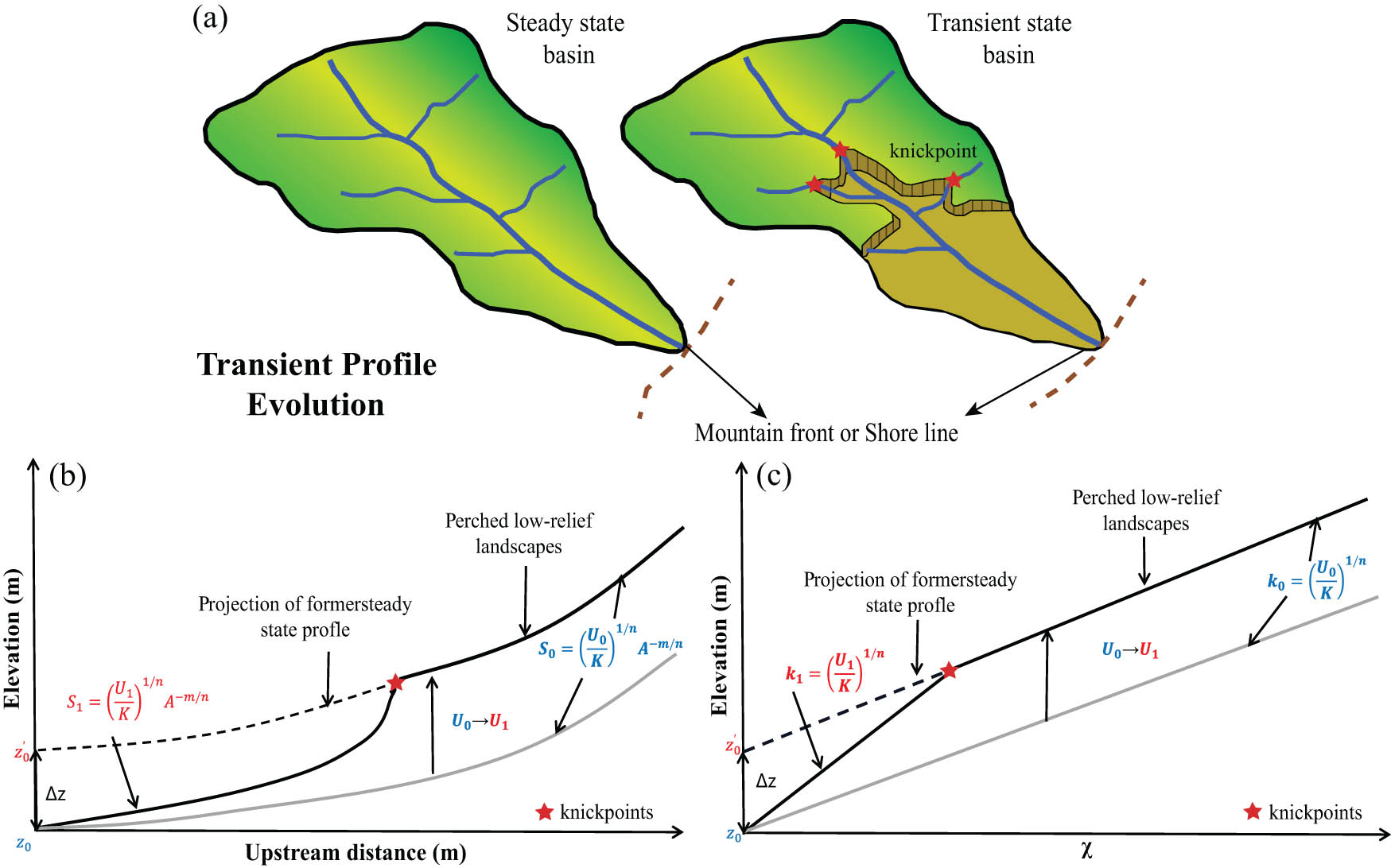
(a) Conceptual model for the evolution of a transient basin from a steady state basin(b) and (c). Schematic diagram of knickpoint trace migration. The present-day river outlet elevation is z
0
, elevation of the projected paleochannel at the outlet is
In this study, we proposed to equip the integral approach with the generalized least squares (GLS) to eliminate residual auto-correlation in the
2 Theoretical background
2.1 Equipping the integral approach with GLSs
We use the GLS method to perform
where
Multiplying equation (6) with ρ and replacing the subscript i with i − 1:
We defined
Compared with equation (6), we find that the slope of the linear fit of
Equation (10) is called the generalized difference equation. It is not in its original form, but rather regresses z on
This transformation is known as the Prais–Winsten transformation [28,29]. After the transformation,
3 Relict channel projection
Knickpoints along a channel profile can be distinguished into two end-member morphologies, i.e. vertical-step and slope-break types ([30]; Figure 2). The former type is defined by a local, discrete increase in channel gradients, which is recognized as a steep elevation drop in river long profile and spikes in slope-area plots (Figure 2a–c). Slope-break knickpoints, on the contrary, are recognized as markers that divide the river long profile into a series of reaches with different channel steepness (Figure 2d–f) [31].
![Figure 2
Classification of knickpoints based on channel profile, slope-area scaling, and Chi-z plot. (a)–(c) illustrate the characteristics of vertical-step knickpoints, while (d)–(f) illustrate the characteristics of slope-break knickpoints (adapted from [30].](/document/doi/10.1515/geo-2025-0900/asset/graphic/j_geo-2025-0900_fig_002.jpg)
Classification of knickpoints based on channel profile, slope-area scaling, and Chi-z plot. (a)–(c) illustrate the characteristics of vertical-step knickpoints, while (d)–(f) illustrate the characteristics of slope-break knickpoints (adapted from [30].
Paleochannel reconstruction deals with the mobile slope-break knickpoint, above which the channel segment is still under steady-state with the previous tectonic uplift rate [26]. We followed the integral approach by Perron and Royden [15], in which the
Using the relict channel concavity (
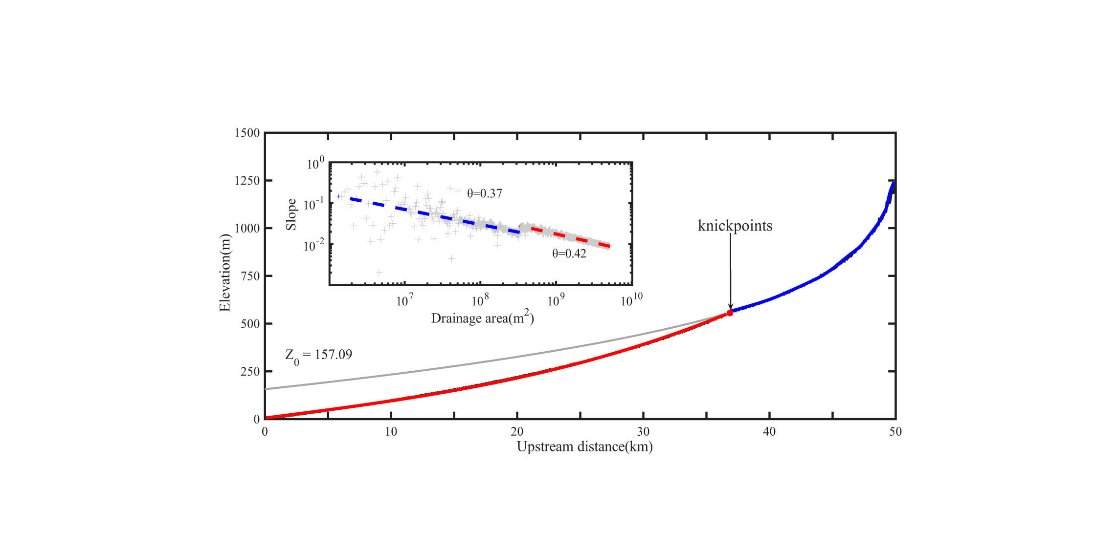
Numerical profile and slope-area data (inset). Parameters: set
4 Case studies
4.1 Numerical cases
We applied the new method to a numerical case to show the importance of using relict channel concavity rather than the reference concavity for re-constructing paleo channel profiles. We first generated a transient profile using the stream-power parameters of channel erodibility
where L is the river total length, x is the upstream distance, and k
a
and h are constants related to river morphology [32,33]. We assumed a steady-state river profile with
Then, we imported an uplift history with an increase in the uplift rates to be
We used both the slope-area analysis method and the integral approach to reconstruct the relict channel profile. The former method, via the smoothing window = 5 and sampling interval = 10 m, resulted in a concavity value of 0.37 and a knickpoint incision depth of about 157.1 m. However, for the noisy elevation data, the integral approach produced relict channel concavity of 0.46 (Figure 4a). Thus, the differences between the estimated and real parameter values may be more attributed to resampling and differentiating elevation data than to elevation noise itself.
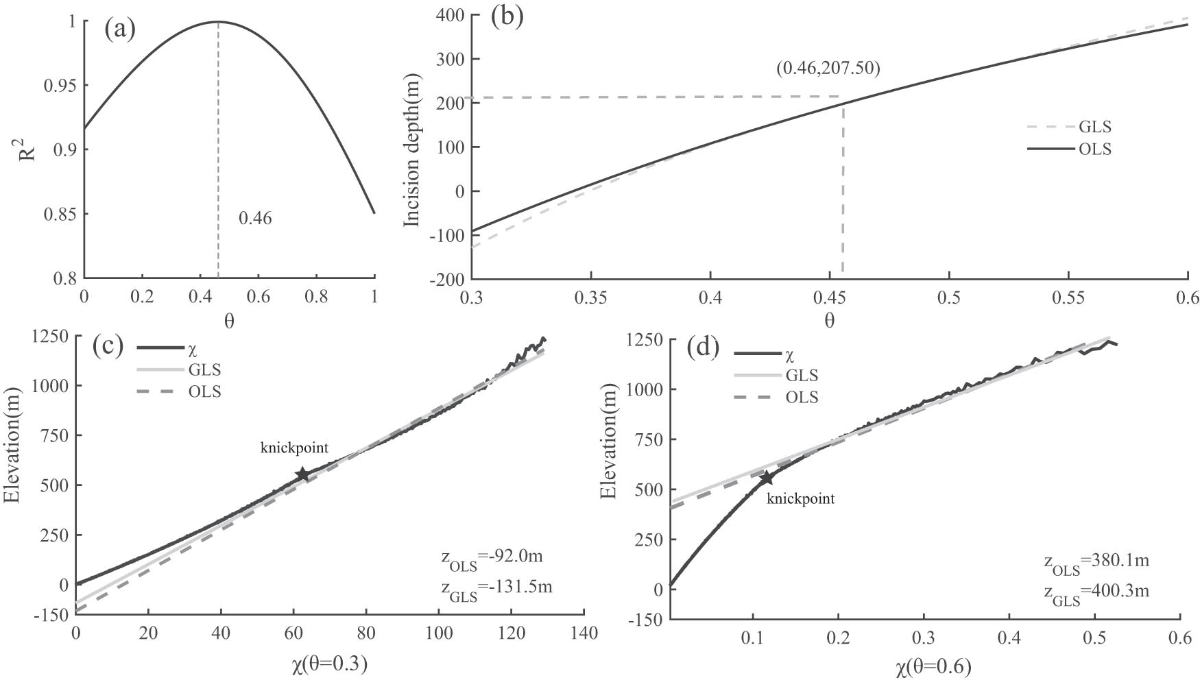
(a) Coefficient of determination (R 2) as a function of concavity, where the peak R² indicates the actual concavity of the river; (b) incision depths calculated by GLS and OLS as the reference concavity varies from 0.3 to 0.6; (c) comparison of chi-z projections of relict channels and calculated incision depths using OLS and GLS for a reference concavity of 0.3 and (d) of 0.6.
Then, based on the integral approach, we utilized a series of reference concavity indices (0.3 and 0.6) to reconstruct the relict profile. We utilized both
4.2 Natural case – mountains bounding the Taiyuan Basin
The Shanxi Rift, well known as the continental rift system, is located in the eastern margin of the Ordos Plateau and is adjacent to the N-S trending Taihang Mountains [34,35,36]. The Taiyuan Basin is situated in the central region of the Shanxi Rift, with the NNE-oriented Taiyue Shan in the east side and Taiyuanxi Shan in the west [37,38,39]. The Taiyuan basin is constrained by two high-angle normal faults, the Jiaocheng Fault in the west side and the Taigu Fault in the east (Figure 5b). The paleomagnetic chronology of the bottom sediment strata in Taiyuan Basin was dated to be about 8.1 Ma, indicating that the basin formed at the late Miocene [40,41]. Wang et al. extracted two transient river channels in the northern tip of the Taiyuanxi Shan and inferred a tectonic history with increases in the uplift rates since the late Miocene [42]. This previous work indicate that the profiles of rivers draining through the mountains bounding the Taiyuan basin can record a history of mountain growth or fault throw at the time scale of more than 106 year and even provide insights into the basin subsidence if considering the case of basin–mountain coupling mechanism. To minimize the influence of the Fenhe River formation and evolution on incision-depth estimates, we used the Fenhe River elevation as the reference base level for its tributaries. In this study, we analyzed 14 rivers in the Taiyuanxi Shan, 6 rivers in the Taiyue Shan, and 17 rivers in the Fenhe River drainage catchment (locations shown in Figure 5b). We analyzed 34 rivers, of which 20 are under steady-state and 14 are characterized by convex-up knickpoints (this analysis is based on the ALOS-12.5 m DEM data). The locations of the knickpoints and the river profiles are shown in Figure 5c. The concavity of the river channels was calculated using both slope-area method and the integral approach equipped with GLS (results are presented in Figure 6).
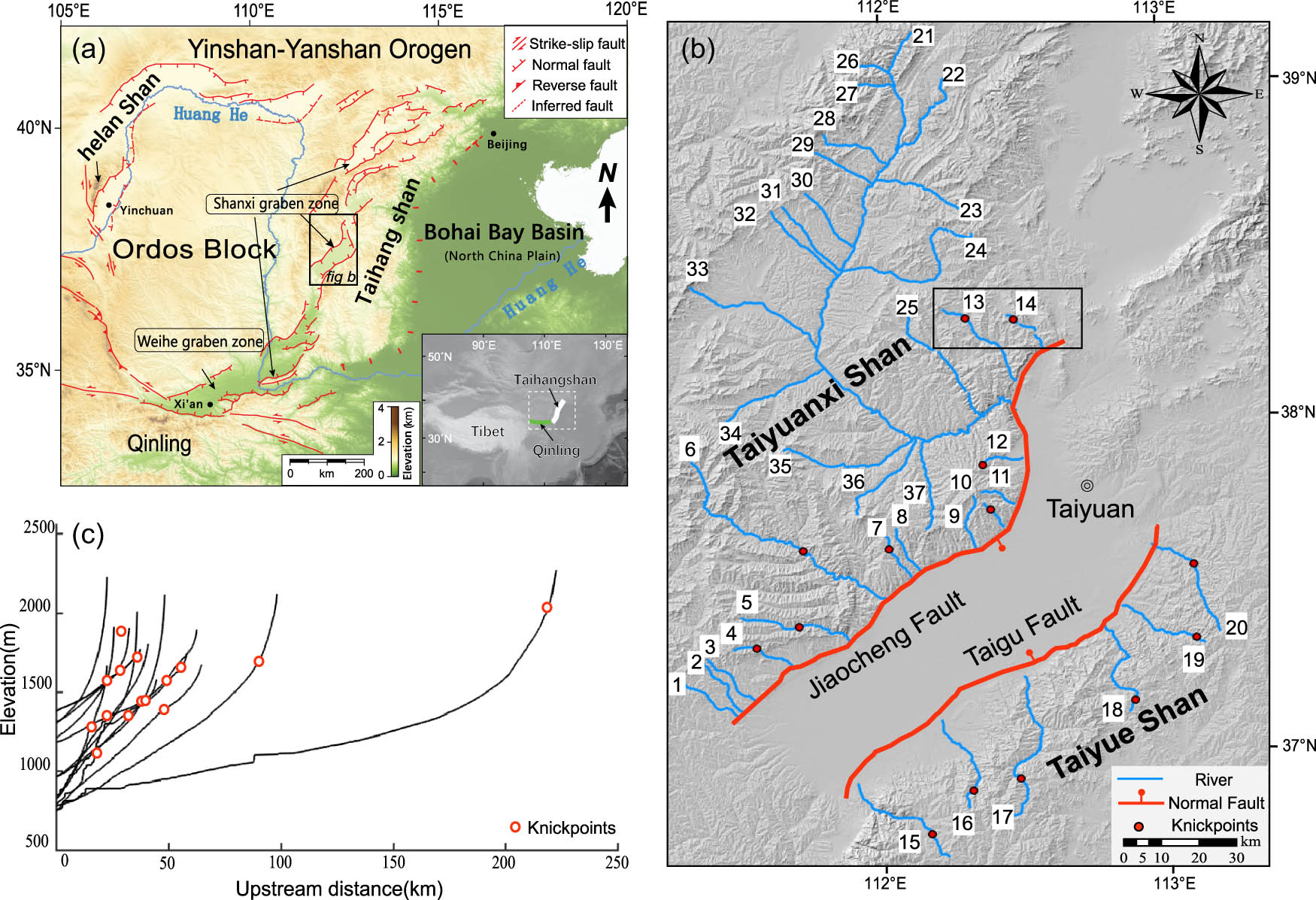
(a) Regional topographic and neotectonic map of North China. Black boxes show the location of the study areas; (b) landforms and rivers around Taiyuan Basin; and (c) river longitudinal profile and location of knickpoints.
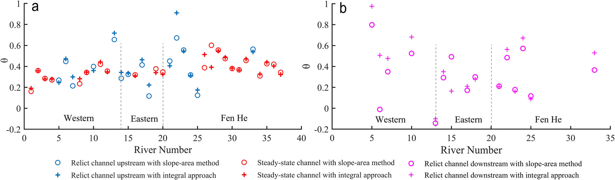
Comparison of results between slope-area analysis and integral approach. (a) Concavity of the steady state channel and the channel upstream of the knickpoint; and (b) the calculated results for the channel below the knickpoints.
Although both methods yield similar concavity index values for steady-state and relict channel profiles, differences are observed for some segments (Figures 6 and 7). Figure 7(a)–(c) shows that, for River 7 on the western side, slope-area analysis produces a concavity of 0.39 and an incision depth of 247.6 m, while our method presents a concavity of 0.3 and an incision depth of 130.5 m. Similarly, for River 17, the slope-area method yields a concavity of 0.42 and an incision depth of 377.4 m, while our method yields a concavity of 0.47 and an incision depth of 367.5 m (Figure 7(d)–(f)). In Figure 7(g)–(i), slope-area analysis on River No. 22 produces a concavity of 0.67 and an incision depth of 92.8 m, while the concavity and incision depth estimated by our method are 0.91 and 136.9 m, respectively.
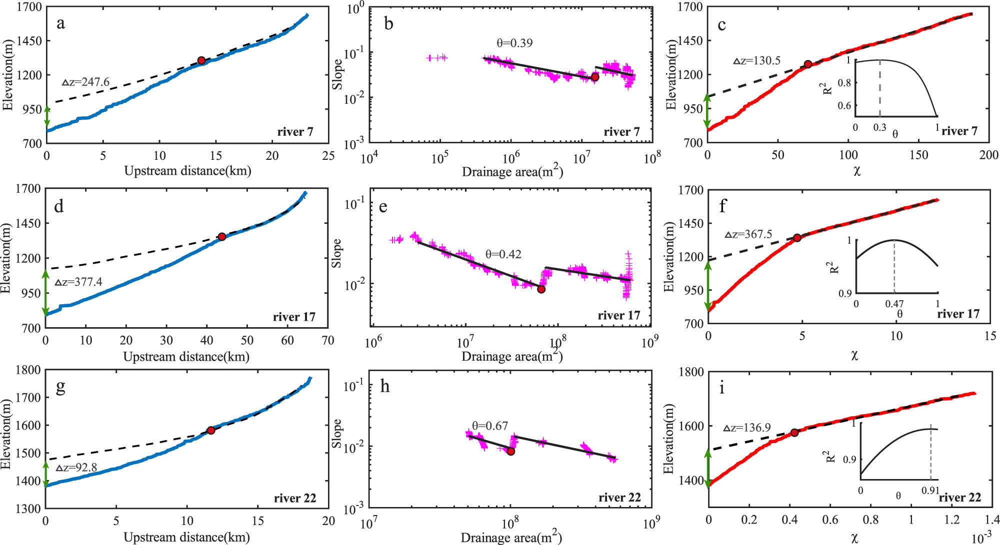
River elevation profile analysis. (a)–(c) Elevation profiles, log-transformed slope–area plot, Chi-plot plots with paleochannel projection for River 7, respectively, and concavity-determination coefficient R 2 plots for calculating the true concavity in the middle and lower panels of (c); (d)–(f) for River 17; (g)–(i) for river 22.
Figure 7 shows that knickpoints on river profiles can cause large scatters in the estimated channel gradients, leading to high uncertainties in the calculated concavity indices. When the slope values are with less scatters (Figure 7(d)–(f)), the slope-area method and the integral approach yield similar results. The integral approach is less influenced by noises in topographic data, which can bring results with higher accuracy relative to the slope-area method.
In addition to slope-break knickpoints, vertical-step types can also affect the concavity calculation when using the slope-area method. As shown in Figure 8a (River No. 27), vertical-step knickpoints cause spikes in the slope-area logarithmic plot. This also demonstrates the impact of DEM quality on concavity calculation, as low-precision DEMs tend to contain numerous similar knickpoints resulting from insufficient accuracy. In Figure 8b and c, we changed the elevation smoothing window and sampling interval to test this effect. The results indicate that the concavities derived from the slope-area method vary a lot as the smoothing window and sampling interval change.
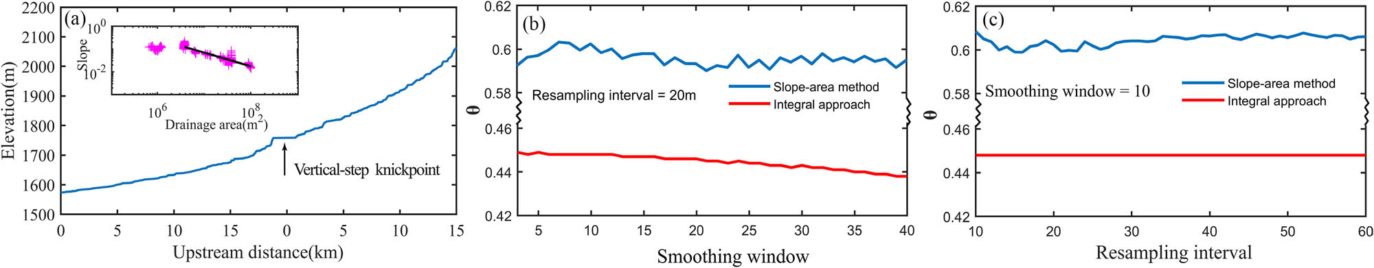
Concavity estimation for River 27, which contains vertical step-like knickpoints. (a) Elevation profile and slope-area logarithmic plot of the river; (b) effect of smoothing window size on concavity calculations using the slope-area method and the integral approach with a fixed resampling interval; and (c) effect of resampling interval on concavity calculations with a fixed smoothing window.
Via both the slope-area method and our
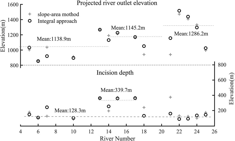
Knickpoint outlet elevation and incision depth in Taiyuan Basin.
5 Discussion
5.1 Influences of smoothing window and re-sampling elevation interval on slope-area analysis
Despite large scatters in the slope dots, the slope-area plot was emphasized for its unique usage in detecting the variations in channel concavity [16]. Theoretical predictions indicate that: (1) a steady-state river should exhibit a smooth concave shape; (2) in the absence of long-wavelength tilting, the concavity of river segments upstream and downstream of a knickpoint should be consistent. However, along real river channels, variations in lithology or landslides and debris flows can lead to departure from theoretical predictions. This is considered to be the reason of large scatters in slope-area plots. However, according to Section 3.1, even for very small elevation noise, resampling and smoothing elevation data can also cause large errors in calculating stream-power parameters. And, there is yet no standard window sizes for smooth and resampling river long profile.
Since in the theistic case, all the parameters can be preset, we used this case to discuss the influences of smoothing and re-sampling windows on calculating slope-area plots and concavity values. First, we fixed the resampling elevation interval at 20 m and changes the smoothing window. Subsequently, we fixed the smoothing window at 10 and varied the resampling interval, with concavity set at 0.46.
The results in Figure 10(a)–(d) show that smaller smoothing windows and resampling intervals lead to greater scatter in slope calculation values. Figure 10e and f further illustrate that parameter changes have a random effect on the concavity calculations, making it difficult to identify an optimal setting. Our conclusions are as follows: (1) resampling interval variations have a greater impact on
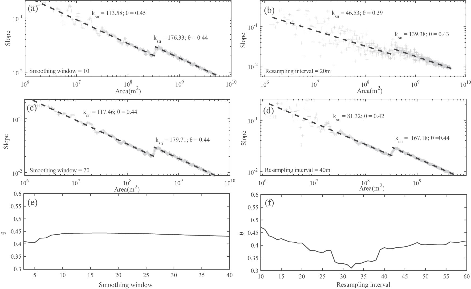
Comparison of results of the slope-area approach. (a) and (c) with no resampling in the plot and smoothing window of 10 and 20; (b) and (d) with no smoothing and resampling intervals of 20 and 40 m, respectively; (e) effect of the smoothing window on the results of concavity calculations; and (f) effect of the results of resampling intervals.
5.2 Residual autocorrelation of
χ
–
z regression
The
To compare the shape of the
![Figure 11
(a) Trend of chi values for the reference concavity, where chi values for all concavities are homogenized to [0, 1]; (b)–(e) effect of OLS versus GLS methods on the computed results, with (b) representing the difference in knickpoint incision depths; (c) the k
sn
ratio, and (e) the effect of the confidence intervals.](/document/doi/10.1515/geo-2025-0900/asset/graphic/j_geo-2025-0900_fig_011.jpg)
(a) Trend of chi values for the reference concavity, where chi values for all concavities are homogenized to [0, 1]; (b)–(e) effect of OLS versus GLS methods on the computed results, with (b) representing the difference in knickpoint incision depths; (c) the k sn ratio, and (e) the effect of the confidence intervals.
The integral approach chooses theta that best fits
Figure 11(e) shows concavity probability distributions with 95% confidence intervals, [0.18, 0.74] for OLS, and [0.27, 0.65] for GLS, indicating that GLS reduces the uncertainty and improves the accuracy of the estimated incision depth. By addressing serial autocorrelation inherent in the integral approach, GLS mitigates accuracy overestimation, resulting in narrower error intervals. Therefore, applying the GLS approach is essential for obtaining accurate estimates of channel concavity and knickpoint incision depth.
5.3 Implications for the subsidence of the Taiyuan Basin
Based on sediment dating from boreholes in the Taiyuan Basin, during the Pliocene (5.8 Ma), the Lvliang Mountains experienced rapid uplift, while the northern section of the Jiaocheng Fault began to activate [43,44]. The faults within the basin controlled much of the subsidence process, leading to a rapid expansion phase of the Taiyuan Basin. In the Early Pleistocene (2.2 Ma), a tectonic stress field transformation occurred, causing the basin’s extension direction to shift from NW-SE to NE-SW [45,46]. This change led to the rapid activity of the NW-SE-trending faults at the front of the Lingshi Uplift, resulting in renewed uplift of the underlying Lingshi Uplift.
We propose that basin subsidence led to the formation of river knickpoints, all of which occurred during the Pliocene. The results of paleochannel reconstruction indicate that the knickpoint incision depths of rivers surrounding the Taiyuan Basin range from 128.3 to 339.7 m, with rivers 13, 14, 15, and 17 having incision depths around 339.7 m. Rivers 13 and 14 are located in the northern Shilingguan Uplift, while rivers 15 and 17 are situated in the southern Lingshi Uplift. The knickpoint incision depth represents a minimum estimate of net surface uplift. Since these knickpoints formed in the early stages of basin formation during the Pliocene, and given that the overall erosion rate of the basin is likely uniform, it suggests that the uplift rate in the uplifted areas is significantly greater than in other regions. Importantly, the high-incision clusters do not coincide systematically with particular lithologic boundaries, implying that lithology exerts only a secondary, local influence on incision [44]. Instead, this finding aligns with structural analysis results, indicating that the Shilingguan and Lingshi uplifts are the areas with the highest regional uplift rates.
6 Conclusions
In this article, we equipped the integral approach with GLSs for relict channel profile re-construction. Via synthetic river profiles generated by numerical modeling, we demonstrate that (1) the difference between channel concavity and reference concavity, and the residual auto-correlation of the
Acknowledgments
We appreciated the Topographic Analysis Kit (TAK) for providing valuable references in analyzing river profiles.
-
Funding information: This study was supported by the National Natural Science Foundation of China (Grant No. 42361144839).
-
Author contributions: Yarong Zhang: writing – original draft, methodology, formal analysis. Yizhou Wang: writing – original draft, project administration, funding acquisition. Hao Xie: writing – original draft, investigation. Chaopeng Li: writing – review & editing, investigation. Huiping Zhang: writing – review & editing.
-
Conflict of interest: The authors declare no conflict of interest.
-
Data availability statement: The data used in this study are available upon reasonable request from the corresponding author. The manuscript has not been submitted to this or any other journal previously.
References
[1] Snyder NP, Whipple KX, Tucker GE, Merritts DJ. Landscape response to tectonic forcing: Digital elevation model analysis of stream profiles in the Mendocino triple junction region, northern California. GSA Bull. 2000;112(8):1250–63.10.1130/0016-7606(2000)112<1250:LRTTFD>2.3.CO;2Search in Google Scholar
[2] Burbank DW, Anderson RS. Tectonic geomorphology. 2nd edn. Environ Eng Geosci. 2013;19(2):198–200.10.2113/gseegeosci.19.2.198Search in Google Scholar
[3] Whipple KX. Bedrock rivers and the geomorphology of active orogens. Annu Rev Earth Planet Sci. 2004;32(1):151–85.10.1146/annurev.earth.32.101802.120356Search in Google Scholar
[4] Crosby BT, Whipple KX. Knickpoint initiation and distribution within fluvial networks: 236 waterfalls in the Waipaoa River, North Island, New Zealand. Geomorphology. 2006;82(1–2):16–38.10.1016/j.geomorph.2005.08.023Search in Google Scholar
[5] Berlin MM, Anderson RS. Modeling of knickpoint retreat on the Roan Plateau, western Colorado. J Geophys Res: Earth Surf. 2007;112(F3):F03S06.10.1029/2006JF000553Search in Google Scholar
[6] Willett SD, McCoy SW, Perron JT, Goren L, Chen C-Y. Dynamic reorganization of river basins. Science. 2014;343(6175):1248765.10.1126/science.1248765Search in Google Scholar
[7] Tarboton DG, Bras RL, Rodriguez-Iturbe I. Scaling and elevation in river networks. Water Resour Res. 1989;25(9):2037–51.10.1029/WR025i009p02037Search in Google Scholar
[8] Whipple KX, Hancock GS, Anderson RS. River incision into bedrock: Mechanics and relative efficacy of plucking, abrasion, and cavitation. GSA Bull. 2000;112(3):490–503.10.1130/0016-7606(2000)112<0490:RIIBMA>2.3.CO;2Search in Google Scholar
[9] Wobus C, Whipple KX, Kirby E, Snyder N, Johnson J, Spyropolou K, et al. Tectonics from topography: Procedures, promise, and pitfalls. Tectonics, climate, and landscape evolution. Vol. 398. Boulder, CO, USA: Geological Society of America; 2006.10.1130/2006.2398(04)Search in Google Scholar
[10] Flint JJ. Stream gradient as a function of order, magnitude, and discharge. Water Resour Res. 1974;10(5):969–73.10.1029/WR010i005p00969Search in Google Scholar
[11] Howard AD, Kerby G. Channel changes in badlands. GSA Bull. 1983;94(6):739–52.10.1130/0016-7606(1983)94<739:CCIB>2.0.CO;2Search in Google Scholar
[12] Howard AD, Dietrich WE, Seidl MA. Modeling fluvial erosion on regional to continental scales. J Geophys Res: Solid Earth. 1994;99(B7):13971–86.10.1029/94JB00744Search in Google Scholar
[13] Kirby E, Whipple K. Quantifying differential rock-uplift rates via stream profile analysis. Geology. 2001;29(5):415–8.10.1130/0091-7613(2001)029<0415:QDRURV>2.0.CO;2Search in Google Scholar
[14] Zhang H, Kirby E, Pitlick J, Anderson RS, Zhang P. Characterizing the transient geomorphic response to base‐level fall in the northeastern Tibetan Plateau. J Geophys Res: Earth Surf. 2017;122(2):546–72.10.1002/2015JF003715Search in Google Scholar
[15] Perron JT, Royden L. An integral approach to bedrock river profile analysis. Earth Surf Process Landf. 2013;38(6):570–6.10.1002/esp.3302Search in Google Scholar
[16] Wang Y, Zhang H, Zheng D, Yu J, Pang J, Ma Y. Coupling slope–area analysis, integral approach and statistic tests to steady-state bedrock river profile analysis. Earth Surf Dyn. 2017;5(1):145–60.10.5194/esurf-5-145-2017Search in Google Scholar
[17] Royden L, Clark M, Whipple K. Evolution of river elevation profiles by bedrock incision: Analytical solutions for transient river profiles related to changing uplift and precipitation rates. Eos Trans Am Geophys Union. 2000;81(48):T62F–09.Search in Google Scholar
[18] Sorby A, England P. Critical assessment of quantitative geomorphology in the footwall of active normal faults, Basin and Range province, western USA. EOS Trans Am Geophys Union. 2004;85:7866219.Search in Google Scholar
[19] Kirby E, Whipple KX. Expression of active tectonics in erosional landscapes. J Struct Geol. 2012;44:54–75.10.1016/j.jsg.2012.07.009Search in Google Scholar
[20] Korup O. Rock-slope failure and the river long profile. Geology. 2006;34(1):45–8.10.1130/G21959.1Search in Google Scholar
[21] Gallen SF, Wegmann KW, Bohnenstieh DR. Miocene rejuvenation of topographic relief in the southern Appalachians. GSA Today. 2013;23(2):4–10.10.1130/GSATG163A.1Search in Google Scholar
[22] Schoenbohm LM, Whipple KX, Burchfiel BC, Chen L. Geomorphic constraints on surface uplift, exhumation, and plateau growth in the Red River region, Yunnan Province, China. GSA Bull. 2004;116(7–8):895–909.10.1130/B25364.1Search in Google Scholar
[23] Clark MK, Mahéo G, Saleeby JB, Farley KA. The non-equilibrium landscape of the southern Sierra Nevada, California. GSA Today. 2005;15:4.10.1130/1052-5173(2005)15[4:TNLOTS]2.0.CO;2Search in Google Scholar
[24] Harkins N, Kirby E, Heimsath A, Robinson R, Reiser U. Transient fluvial incision in the headwaters of the Yellow River, northeastern Tibet, China. J Geophys Res: Earth Surf. 2007;112(F3):F03S04.10.1029/2006JF000570Search in Google Scholar
[25] Duvall A, Kirby E, Burbank D. Tectonic and lithologic controls on bedrock channel profiles and processes in coastal California. J Geophys Res: Earth Surf. 2004;109(F3):F03002.10.1029/2003JF000086Search in Google Scholar
[26] Niemann JD, Gasparini NM, Tucker GE, Bras R. Landforms. A quantitative evaluation of Playfair’s law and its use in testing long‐term stream erosion models. Earth Surf Process Landf. 2001;26(12)1317–32.10.1002/esp.272Search in Google Scholar
[27] Kirby E, Whipple KX, Tang W, Chen Z. Distribution of active rock uplift along the eastern margin of the Tibetan Plateau: Inferences from bedrock channel longitudinal profiles. J Geophys Res: Solid Earth. 2003;108(B4):2217.10.1029/2001JB000861Search in Google Scholar
[28] Prais SJ, Winsten CB. Trend estimators and serial correlation. Chicago, IL: Cowles Commission (Discussion Paper No. 383); 1954.Search in Google Scholar
[29] Hamilton JD. Chapter 50 State-space models. Handbook of econometrics. Vol. 4. Amsterdam, Netherlands: Elsevier; 1994. p. 3039–80.10.1016/S1573-4412(05)80019-4Search in Google Scholar
[30] Haviv I, Enzel Y, Whipple KX, Zilberman E, Matmon A, Stone J, et al. Evolution of vertical knickpoints (waterfalls) with resistant caprock: Insights from numerical modeling. J Geophys Res: Earth Surf. 2010;115(F3):F03028.10.1029/2008JF001187Search in Google Scholar
[31] Whipple KX. The influence of climate on the tectonic evolution of mountain belts. Nat Geosci. 2009;2(2):97–104.10.1038/ngeo413Search in Google Scholar
[32] Hack JT. Studies of longitudinal stream profiles in Virginia and Maryland. Washington, D.C.: U.S. Government Printing Office; Report. 1957. Report No.: 294B.10.3133/pp294BSearch in Google Scholar
[33] Sassolas-Serrayet T, Cattin R, Ferry M. The shape of watersheds. Nat Commun. 2018;9(1):3791.10.1038/s41467-018-06210-4Search in Google Scholar
[34] Chen G. On the geotectonic nature of the Fen-Wei rift system. Tectonophysics. 1987;143(1):217–23.10.1016/0040-1951(87)90091-6Search in Google Scholar
[35] Xu X, Ma X, Deng Q. Neotectonic activity along the Shanxi rift system, China. Tectonophysics. 1993;219(4):305–25.10.1016/0040-1951(93)90180-RSearch in Google Scholar
[36] Clinkscales C, Kapp PA, Wang H. Exhumation history of the north-central Shanxi Rift, North China, revealed by low-temperature thermochronology. Earth Planet Sci Lett. 2020;536:116146.10.1016/j.epsl.2020.116146Search in Google Scholar
[37] Xu Y, Yue L, Yue L, Li J, Li J, Sun L, et al. An 11-Ma-old red clay sequence on the Eastern Chinese Loess Plateau. Palaeogeogr, Palaeoclimatol, Palaeoecol. 2009;284:383–91.10.1016/j.palaeo.2009.10.023Search in Google Scholar
[38] Shi W, Dong S, Hu J. Neotectonics around the Ordos Block, North China: A review and new insights. Earth-Sci Rev. 2020;200:102969.10.1016/j.earscirev.2019.102969Search in Google Scholar
[39] Chen X, Dong S, Shi W, Zuza AV, Li Z, Chen P, et al. Magnetostratigraphic ages of the Cenozoic Weihe and Shanxi Grabens in North China and their tectonic implications. Tectonophysics. 2021;813:228914.10.1016/j.tecto.2021.228914Search in Google Scholar
[40] Yin A. Cenozoic tectonic evolution of Asia: A preliminary synthesis. Tectonophysics. 2010;488(1–4):293–325.10.1016/j.tecto.2009.06.002Search in Google Scholar
[41] Wei R, Zhuang Q, Yan J, Wei Y, Du Y, Fan J. Late Cenozoic stratigraphic division and sedimentary environment of Jinzhong Basin in Shanxi Province, with the climate and lake evolution since the pre-Qin period (2500 years ago). Geol China. 2022;49(3):912–28.Search in Google Scholar
[42] Wang Y, Zheng D, Zhang H. The methods and program implementation for river longitudinal profile analysis—RiverProAnalysis, a set of open-source functions based on the Matlab platform. Sci China Earth Sci. 2022;65(9):1788–809.10.1007/s11430-021-9938-xSearch in Google Scholar
[43] Pan F, Li J, Xu Y, Wingate MTD, Yue L, Li Y, et al. Uplift of the lüliang mountains at ca. 5.7 Ma: Insights from provenance of the Neogene eolian red clay of the eastern Chinese Loess Plateau. Palaeogeogr Palaeoclimatol Palaeoecol. 2018;502:63–73.10.1016/j.palaeo.2018.04.024Search in Google Scholar
[44] Zhuang Q, Wei R, He H. Depositional record and geochemistry constraints on the late miocene–quaternary evolution of the taiyuan basin in shanxi rift system, China. Front Earth Sci. 2022;10:833585.10.3389/feart.2022.833585Search in Google Scholar
[45] Wang M, Shen Z-K. Present-day crustal deformation of continental china derived from GPS and its tectonic implications. J Geophys Res: Solid Earth. 2020;125(2):e2019JB018774.10.1029/2019JB018774Search in Google Scholar
[46] Ao H, Rohling EJ, Zhang R, Roberts AP, Holbourn AE, Ladant J-B, et al. Global warming-induced Asian hydrological climate transition across the Miocene–Pliocene boundary. Nat Commun. 2021;12(1):6935.10.1038/s41467-021-27054-5Search in Google Scholar PubMed PubMed Central
© 2025 the author(s), published by De Gruyter
This work is licensed under the Creative Commons Attribution 4.0 International License.
Articles in the same Issue
- Research Articles
- Seismic response and damage model analysis of rocky slopes with weak interlayers
- Multi-scenario simulation and eco-environmental effect analysis of “Production–Living–Ecological space” based on PLUS model: A case study of Anyang City
- Remote sensing estimation of chlorophyll content in rape leaves in Weibei dryland region of China
- GIS-based frequency ratio and Shannon entropy modeling for landslide susceptibility mapping: A case study in Kundah Taluk, Nilgiris District, India
- Natural gas origin and accumulation of the Changxing–Feixianguan Formation in the Puguang area, China
- Spatial variations of shear-wave velocity anomaly derived from Love wave ambient noise seismic tomography along Lembang Fault (West Java, Indonesia)
- Evaluation of cumulative rainfall and rainfall event–duration threshold based on triggering and non-triggering rainfalls: Northern Thailand case
- Pixel and region-oriented classification of Sentinel-2 imagery to assess LULC dynamics and their climate impact in Nowshera, Pakistan
- The use of radar-optical remote sensing data and geographic information system–analytical hierarchy process–multicriteria decision analysis techniques for revealing groundwater recharge prospective zones in arid-semi arid lands
- Effect of pore throats on the reservoir quality of tight sandstone: A case study of the Yanchang Formation in the Zhidan area, Ordos Basin
- Hydroelectric simulation of the phreatic water response of mining cracked soil based on microbial solidification
- Spatial-temporal evolution of habitat quality in tropical monsoon climate region based on “pattern–process–quality” – a case study of Cambodia
- Early Permian to Middle Triassic Formation petroleum potentials of Sydney Basin, Australia: A geochemical analysis
- Micro-mechanism analysis of Zhongchuan loess liquefaction disaster induced by Jishishan M6.2 earthquake in 2023
- Prediction method of S-wave velocities in tight sandstone reservoirs – a case study of CO2 geological storage area in Ordos Basin
- Ecological restoration in valley area of semiarid region damaged by shallow buried coal seam mining
- Hydrocarbon-generating characteristics of Xujiahe coal-bearing source rocks in the continuous sedimentary environment of the Southwest Sichuan
- Hazard analysis of future surface displacements on active faults based on the recurrence interval of strong earthquakes
- Structural characterization of the Zalm district, West Saudi Arabia, using aeromagnetic data: An approach for gold mineral exploration
- Research on the variation in the Shields curve of silt initiation
- Reuse of agricultural drainage water and wastewater for crop irrigation in southeastern Algeria
- Assessing the effectiveness of utilizing low-cost inertial measurement unit sensors for producing as-built plans
- Analysis of the formation process of a natural fertilizer in the loess area
- Machine learning methods for landslide mapping studies: A comparative study of SVM and RF algorithms in the Oued Aoulai watershed (Morocco)
- Chemical dissolution and the source of salt efflorescence in weathering of sandstone cultural relics
- Molecular simulation of methane adsorption capacity in transitional shale – a case study of Longtan Formation shale in Southern Sichuan Basin, SW China
- Evolution characteristics of extreme maximum temperature events in Central China and adaptation strategies under different future warming scenarios
- Estimating Bowen ratio in local environment based on satellite imagery
- 3D fusion modeling of multi-scale geological structures based on subdivision-NURBS surfaces and stratigraphic sequence formalization
- Comparative analysis of machine learning algorithms in Google Earth Engine for urban land use dynamics in rapidly urbanizing South Asian cities
- Study on the mechanism of plant root influence on soil properties in expansive soil areas
- Simulation of seismic hazard parameters and earthquakes source mechanisms along the Red Sea rift, western Saudi Arabia
- Tectonics vs sedimentation in foredeep basins: A tale from the Oligo-Miocene Monte Falterona Formation (Northern Apennines, Italy)
- Investigation of landslide areas in Tokat-Almus road between Bakımlı-Almus by the PS-InSAR method (Türkiye)
- Predicting coastal variations in non-storm conditions with machine learning
- Cross-dimensional adaptivity research on a 3D earth observation data cube model
- Geochronology and geochemistry of late Paleozoic volcanic rocks in eastern Inner Mongolia and their geological significance
- Spatial and temporal evolution of land use and habitat quality in arid regions – a case of Northwest China
- Ground-penetrating radar imaging of subsurface karst features controlling water leakage across Wadi Namar dam, south Riyadh, Saudi Arabia
- Rayleigh wave dispersion inversion via modified sine cosine algorithm: Application to Hangzhou, China passive surface wave data
- Fractal insights into permeability control by pore structure in tight sandstone reservoirs, Heshui area, Ordos Basin
- Debris flow hazard characteristic and mitigation in Yusitong Gully, Hengduan Mountainous Region
- Research on community characteristics of vegetation restoration in hilly power engineering based on multi temporal remote sensing technology
- Identification of radial drainage networks based on topographic and geometric features
- Trace elements and melt inclusion in zircon within the Qunji porphyry Cu deposit: Application to the metallogenic potential of the reduced magma-hydrothermal system
- Pore, fracture characteristics and diagenetic evolution of medium-maturity marine shales from the Silurian Longmaxi Formation, NE Sichuan Basin, China
- Study of the earthquakes source parameters, site response, and path attenuation using P and S-waves spectral inversion, Aswan region, south Egypt
- Source of contamination and assessment of potential health risks of potentially toxic metal(loid)s in agricultural soil from Al Lith, Saudi Arabia
- Regional spatiotemporal evolution and influencing factors of rural construction areas in the Nanxi River Basin via GIS
- An efficient network for object detection in scale-imbalanced remote sensing images
- Effect of microscopic pore–throat structure heterogeneity on waterflooding seepage characteristics of tight sandstone reservoirs
- Environmental health risk assessment of Zn, Cd, Pb, Fe, and Co in coastal sediments of the southeastern Gulf of Aqaba
- A modified Hoek–Brown model considering softening effects and its applications
- Evaluation of engineering properties of soil for sustainable urban development
- The spatio-temporal characteristics and influencing factors of sustainable development in China’s provincial areas
- Application of a mixed additive and multiplicative random error model to generate DTM products from LiDAR data
- Gold vein mineralogy and oxygen isotopes of Wadi Abu Khusheiba, Jordan
- Prediction of surface deformation time series in closed mines based on LSTM and optimization algorithms
- 2D–3D Geological features collaborative identification of surrounding rock structural planes in hydraulic adit based on OC-AINet
- Spatiotemporal patterns and drivers of Chl-a in Chinese lakes between 1986 and 2023
- Land use classification through fusion of remote sensing images and multi-source data
- Nexus between renewable energy, technological innovation, and carbon dioxide emissions in Saudi Arabia
- Analysis of the spillover effects of green organic transformation on sustainable development in ethnic regions’ agriculture and animal husbandry
- Factors impacting spatial distribution of black and odorous water bodies in Hebei
- Large-scale shaking table tests on the liquefaction and deformation responses of an ultra-deep overburden
- Impacts of climate change and sea-level rise on the coastal geological environment of Quang Nam province, Vietnam
- Reservoir characterization and exploration potential of shale reservoir near denudation area: A case study of Ordovician–Silurian marine shale, China
- Seismic prediction of Permian volcanic rock reservoirs in Southwest Sichuan Basin
- Application of CBERS-04 IRS data to land surface temperature inversion: A case study based on Minqin arid area
- Geological characteristics and prospecting direction of Sanjiaoding gold mine in Saishiteng area
- Research on the deformation prediction model of surrounding rock based on SSA-VMD-GRU
- Geochronology, geochemical characteristics, and tectonic significance of the granites, Menghewula, Southern Great Xing’an range
- Hazard classification of active faults in Yunnan base on probabilistic seismic hazard assessment
- Characteristics analysis of hydrate reservoirs with different geological structures developed by vertical well depressurization
- Estimating the travel distance of channelized rock avalanches using genetic programming method
- Landscape preferences of hikers in Three Parallel Rivers Region and its adjacent regions by content analysis of user-generated photography
- New age constraints of the LGM onset in the Bohemian Forest – Central Europe
- Characteristics of geological evolution based on the multifractal singularity theory: A case study of Heyu granite and Mesozoic tectonics
- Soil water content and longitudinal microbiota distribution in disturbed areas of tower foundations of power transmission and transformation projects
- Oil accumulation process of the Kongdian reservoir in the deep subsag zone of the Cangdong Sag, Bohai Bay Basin, China
- Investigation of velocity profile in rock–ice avalanche by particle image velocimetry measurement
- Optimizing 3D seismic survey geometries using ray tracing and illumination modeling: A case study from Penobscot field
- Sedimentology of the Phra That and Pha Daeng Formations: A preliminary evaluation of geological CO2 storage potential in the Lampang Basin, Thailand
- Improved classification algorithm for hyperspectral remote sensing images based on the hybrid spectral network model
- Map analysis of soil erodibility rates and gully erosion sites in Anambra State, South Eastern Nigeria
- Identification and driving mechanism of land use conflict in China’s South-North transition zone: A case study of Huaihe River Basin
- Evaluation of the impact of land-use change on earthquake risk distribution in different periods: An empirical analysis from Sichuan Province
- A test site case study on the long-term behavior of geotextile tubes
- An experimental investigation into carbon dioxide flooding and rock dissolution in low-permeability reservoirs of the South China Sea
- Detection and semi-quantitative analysis of naphthenic acids in coal and gangue from mining areas in China
- Comparative effects of olivine and sand on KOH-treated clayey soil
- YOLO-MC: An algorithm for early forest fire recognition based on drone image
- Earthquake building damage classification based on full suite of Sentinel-1 features
- Potential landslide detection and influencing factors analysis in the upper Yellow River based on SBAS-InSAR technology
- Assessing green area changes in Najran City, Saudi Arabia (2013–2022) using hybrid deep learning techniques
- An advanced approach integrating methods to estimate hydraulic conductivity of different soil types supported by a machine learning model
- Hybrid methods for land use and land cover classification using remote sensing and combined spectral feature extraction: A case study of Najran City, KSA
- Streamlining digital elevation model construction from historical aerial photographs: The impact of reference elevation data on spatial accuracy
- Analysis of urban expansion patterns in the Yangtze River Delta based on the fusion impervious surfaces dataset
- A metaverse-based visual analysis approach for 3D reservoir models
- Late Quaternary record of 100 ka depositional cycles on the Larache shelf (NW Morocco)
- Integrated well-seismic analysis of sedimentary facies distribution: A case study from the Mesoproterozoic, Ordos Basin, China
- Study on the spatial equilibrium of cultural and tourism resources in Macao, China
- Urban road surface condition detecting and integrating based on the mobile sensing framework with multi-modal sensors
- Application of improved sine cosine algorithm with chaotic mapping and novel updating methods for joint inversion of resistivity and surface wave data
- The synergistic use of AHP and GIS to assess factors driving forest fire potential in a peat swamp forest in Thailand
- Dynamic response analysis and comprehensive evaluation of cement-improved aeolian sand roadbed
- Rock control on evolution of Khorat Cuesta, Khorat UNESCO Geopark, Northeastern Thailand
- Gradient response mechanism of carbon storage: Spatiotemporal analysis of economic-ecological dimensions based on hybrid machine learning
- Comparison of several seismic active earth pressure calculation methods for retaining structures
- Mantle dynamics and petrogenesis of Gomer basalts in the Northwestern Ethiopia: A geochemical perspective
- Study on ground deformation monitoring in Xiong’an New Area from 2021 to 2023 based on DS-InSAR
- Paleoenvironmental characteristics of continental shale and its significance to organic matter enrichment: Taking the fifth member of Xujiahe Formation in Tianfu area of Sichuan Basin as an example
- Equipping the integral approach with generalized least squares to reconstruct relict channel profile and its usage in the Shanxi Rift, northern China
- InSAR-driven landslide hazard assessment along highways in hilly regions: A case-based validation approach
- Attribution analysis of multi-temporal scale surface streamflow changes in the Ganjiang River based on a multi-temporal Budyko framework
- Review Articles
- Humic substances influence on the distribution of dissolved iron in seawater: A review of electrochemical methods and other techniques
- Applications of physics-informed neural networks in geosciences: From basic seismology to comprehensive environmental studies
- Ore-controlling structures of granite-related uranium deposits in South China: A review
- Shallow geological structure features in Balikpapan Bay East Kalimantan Province – Indonesia
- A review on the tectonic affinity of microcontinents and evolution of the Proto-Tethys Ocean in Northeastern Tibet
- Special Issue: Natural Resources and Environmental Risks: Towards a Sustainable Future - Part II
- Depopulation in the Visok micro-region: Toward demographic and economic revitalization
- Special Issue: Geospatial and Environmental Dynamics - Part II
- Advancing urban sustainability: Applying GIS technologies to assess SDG indicators – a case study of Podgorica (Montenegro)
- Spatiotemporal and trend analysis of common cancers in men in Central Serbia (1999–2021)
- Minerals for the green agenda, implications, stalemates, and alternatives
- Spatiotemporal water quality analysis of Vrana Lake, Croatia
- Functional transformation of settlements in coal exploitation zones: A case study of the municipality of Stanari in Republic of Srpska (Bosnia and Herzegovina)
- Hypertension in AP Vojvodina (Northern Serbia): A spatio-temporal analysis of patients at the Institute for Cardiovascular Diseases of Vojvodina
- Regional patterns in cause-specific mortality in Montenegro, 1991–2019
- Spatio-temporal analysis of flood events using GIS and remote sensing-based approach in the Ukrina River Basin, Bosnia and Herzegovina
- Flash flood susceptibility mapping using LiDAR-Derived DEM and machine learning algorithms: Ljuboviđa case study, Serbia
- Geocultural heritage as a basis for geotourism development: Banjska Monastery, Zvečan (Serbia)
- Assessment of groundwater potential zones using GIS and AHP techniques – A case study of the zone of influence of Kolubara Mining Basin
- Impact of the agri-geographical transformation of rural settlements on the geospatial dynamics of soil erosion intensity in municipalities of Central Serbia
- Where faith meets geomorphology: The cultural and religious significance of geodiversity explored through geospatial technologies
- Applications of local climate zone classification in European cities: A review of in situ and mobile monitoring methods in urban climate studies
- Complex multivariate water quality impact assessment on Krivaja River
- Ionization hotspots near waterfalls in Eastern Serbia’s Stara Planina Mountain
- Shift in landscape use strategies during the transition from the Bronze age to Iron age in Northwest Serbia
- Assessing the geotourism potential of glacial lakes in Plav, Montenegro: A multi-criteria assessment by using the M-GAM model
- Flash flood potential index at national scale: Susceptibility assessment within catchments