Gradient response mechanism of carbon storage: Spatiotemporal analysis of economic-ecological dimensions based on hybrid machine learning
-
Xuankai Huang
 ,
Binjie Zhou
,
Binjie Zhou

Abstract
To explore the mechanisms of spatiotemporal changes in carbon storage (CS) and identify optimal pathways for achieving carbon neutrality. Existing studies have revealed the intrinsic relationship between land use changes and carbon storage. However, research gaps remain regarding the spatiotemporal driving mechanisms of CS in urban agglomerations from an economic-ecological gradient perspective. This study integrates a hybrid machine learning framework (coupling Categorical boosting-Shapley Additive exPlanations and GeoDetector based on optimal parameters-Wavelet analysis) to construct a tripartite CS assessment system encompassing “gradient analysis-scenario simulation-mechanism identification.” Based on the Technique for Order Preference by Similarity to Ideal Solution method, multi-gradient spatial units in the Yangtze River Delta were delineated. The PLUS-InVEST model was employed to simulate the spatiotemporal evolution of CS under business as usual, cultivated-land protection, and ecological protection (ELC) scenarios from 2030 to 2060, thereby revealing the gradient response mechanisms in ecological governance of territorial space. The findings indicate that (1) from the gradient difference dimension, the expansion of built land from 2000 to 2020 led to a continuous decline in CS, with the decline intensity in high-economic-gradient zones exceeding that in high-ecological-gradient zones, primarily due to significant reductions in forest and arable land in high-economic-gradient areas. (2) Spatiotemporal coupling characteristics revealed an increasing coastal-inland gradient and a decreasing north-south gradient. The fluctuation coefficient of CS in high-economic-gradient zones was 50% higher than in ecological zones. (3) Mechanism analysis demonstrated that natural factors (digital elevation model, slope) exerted decisive explanatory power over CS changes within gradient zones, while the nighttime light index exhibited a secondary driving effect in high-economic-gradient zones. Multi-model validation indicated that ecological governance policies could effectively trigger “gradient transitions” in CS by enhancing the interaction effects between net primary productivity and topographic factors. The proposed multi-gradient machine learning analytical framework provides a decision-making pathway of “gradient diagnosis-process simulation-policy response” for coordinated CS management in urban agglomerations and ecological governance of territorial space.
1 Introduction
Global climate change has emerged as one of the most severe challenges of the twenty-first century [1]. The IPCC Sixth Assessment Report unequivocally states that the increase in atmospheric greenhouse gas concentrations caused by human activities is the primary driver of climate change, emphasizing that reducing carbon emissions and enhancing carbon sequestration capacity are critical measures for climate change mitigation [2]. Urbanization is a major driver of global land use changes and carbon (LUCC) and carbon emissions, with continuous urban expansion leading to catastrophic losses in terrestrial ecosystems [3]. Research indicates that terrestrial ecosystems offset approximately 30% of global carbon emissions [4], making their protection and restoration indispensable for achieving carbon neutrality targets. As the world’s largest developing country in terms of carbon emissions, China accounts for over 27% of global emissions. In response, China has actively addressed the challenges of global climate change, pledging to peak carbon emissions before 2030 and achieve carbon neutrality by 2060 [5]. It is evident that increasing carbon storage (CS) in Earth’s ecosystems and reducing carbon emissions have become a global consensus for sustainable development [6].
China needs to balance ecological and socio-economic sustainable development, exploring pathways to achieve the “Dual Carbon Goals” at low cost [7,8,9]. In previous studies, researchers have investigated the spatial characteristics, driving mechanisms, and management approaches of ecological CS across multiple scales, including administrative regions, economic belts, watersheds, and grids [10,11]. Additionally, some scholars have examined the impact patterns of CS changes during the development of typical cities [12]. Concurrently, field surveys and model simulations have been conducted to explore the dynamic variations in CS and their driving factors in different ecosystems [13]. Various natural and anthropogenic drivers exert significant influences on terrestrial CS. Natural factors include climate [14] and geographical environment [15], while anthropogenic factors encompass socio-economic development [16] and restoration management [17]. These factors interact to form a complex network affecting CS [18]. Such research has enhanced the understanding of the impacts of natural and anthropogenic factors on CS, which is crucial for avoiding conflicts between economic development and ecosystem services [19,20]. Studies on CS within ecosystems often leverage established correlations between LUCC types and their respective carbon densities [21], focusing on how land conversion influences CS trends [22]. These correlations are particularly significant when applied to simulate CS across different scales and temporal dimensions [23,24]. Based on this, researchers have developed and coupled various models for LUCC and CS prediction and assessment, addressing diverse scales and perspectives.
Exploring the dynamic relationship between urbanization and the ecological environment is essential for understanding CS. Existing studies have analyzed the impacts of climate change, LUCC, and human activities on regional CS [25]. China is the fastest urbanizing country in the world, and the Yangtze River Delta (YRD) region is one of the key areas of urbanization in China, exhibiting significant spatial gradient differences in ecological and socio-economic foundations [26,27]. The development of urban agglomerations greatly influences CS changes, and CS may also display high spatial heterogeneity along urban agglomeration gradients [24,28]. On one hand, human activities such as urban expansion and infrastructure construction lead to the reduction and fragmentation of natural ecosystems, diminishing ecosystem service functions [29]. On the other hand, increasing energy consumption and carbon emissions, coupled with insufficient carbon sequestration capacity, have intensified the trilemma of “ecological protection-economic development-carbon neutrality [30,31].” Regional coordinated development policies, such as those for urban agglomerations, metropolitan areas, and economic belts, have been implemented as critical national strategies in China [32], emphasizing collaborative management of economic development and territorial ecological protection. Similarly, CS management should also be conducted at a regional scale, aligned with economic development and ecological conservation efforts [33]. Therefore, it is necessary to break through the traditional research on spatial heterogeneity from the perspective of regional gradient differentiation of typical urban agglomerations, and construct a comprehensive evaluation framework that takes into account social economy, CS and ecological protection based on the “gradient theory” [34,35], to clarify the changes and driving mechanisms of CS in different economic and ecological gradient zones, and to deeply study the gradient response mechanism of CS.
This study addresses unresolved research questions based on recent findings. (1) How do the fluctuations in LUCC and CS across the study area and its gradient zones differ between the period of rapid economic development (2000–2020) and the Dual Carbon Goals years (2030 and 2060)? (2) Within the gradient zones, how do driving factors influence the spatiotemporal dynamics of CS? What are the driving characteristics and mechanisms? (3) How does gradient zone differentiation affect the spatial heterogeneity of CS? (4) What are the development priorities for each gradient zone, and what is the synergistic development model for economy, ecology, and CS? This study takes the Yangtze River Delta (YRD) region as a research case, introduces Forman’s landscape gradient theory [36], incorporates the social and economic index system based on its ecological assessment indicators, divides the economic and ecological gradient zones of the YRD region through the Technique for Order Preference by Similarity to Ideal Solution (TOPSIS) method, and constructs a “multi-scale-gradient” composite analysis framework. The PLUS-InVEST model was applied to predict LUCC and CS under multiple scenarios for 2030 and 2060. Additionally, the Categorical boosting (CatBoost)-Shapley Additive exPlanations (SHAP) and GeoDetector based on optimal parameters (OPGD)-WA models were utilized to analyze the driving characteristics and spatial heterogeneity of CS changes from 2020 to 2060 across the entire region and gradient zones under three scenarios: Business as usual (BAU), cultivated-land protection (CP), and ELC. The study proposes a gradient-based collaborative optimization pathway to reconcile conflicts among the dual carbon goals, national territorial spatial ecological governance, and socioeconomic development. It offers novel insights into achieving a low-carbon ecology for sustainable development.
2 Study area and data
2.1 Study area
The YRD (27°02′N–35°20′N, 114°25′E–121°57′E) encompasses Shanghai, Jiangsu, Zhejiang, and Anhui provinces, comprising 41 cities (Figure 1). Spanning 35.80 × 10⁴ km2. This region features dense river networks, intricate coastlines, and a subtropical monsoon climate, with terrain sloping westward and southward. Its abundant lakes, rivers, and high forest coverage establish it as a critical ecological security barrier [27]. In 2019, the region generated a gross domestic product (GDP) of 23.72 trillion yuan (24% of China’s total) with 71.1% urbanization, ranking as the world’s sixth-largest urban agglomeration and a pivotal economic hub. Despite its national strategic status in regional integration, rapid growth has intensified environmental pollution and carbon emissions typical of megacity clusters [37]. Addressing declining ecological quality and carrying capacity, analyzing CS dynamics and drivers is urgently needed. Such efforts can optimize socioeconomic, ecological, and land resource allocation, enhance gradient-based coordination between development and CS conservation, and promote sustainable socio-ecological balance, key to achieving low-carbon transitions.
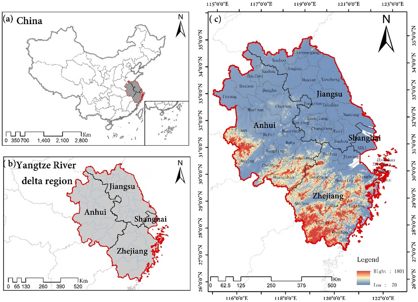
Geographic location of YRD City. (a) Administrative regions of China; (b) provincial administrative units in the Yangtze River Delta; and (c) study the municipal-level units and basic geographical features of the research area.
2.2 Data source and processing
The LUCC data have a resolution of 30 m, and the LUCC data for the years 2000, 2010, and 2020 in the study area were selected. Based on the primary land classification standard, the land types in the YRD region were categorized into six classes: cultivated land (CL), woodland (WL), grassland (GL), water (W), unused land (UL), and built land. The YRD region is vast, with significant spatial heterogeneity in natural ecological environments and socio-economic development across local areas. Therefore, 24 change-driving factors were selected from three dimensions: surface, meteorology, and human activities. Additionally, five key ecological constraint factors were chosen, totaling 29 factor datasets. The specific information and sources of the data are provided in Table 1 and Figure 2. To ensure consistency in the resolution and scale of the factor data, all datasets were uniformly resampled to a resolution of 90 m × 90 m and projected using the WGS_1984_UTM_Zone_50N coordinate system to maintain data correspondence.
Basic data information
| Data type | Data name | Year | Precision (m) | Data source |
|---|---|---|---|---|
| LUCC data | LUCC | 2000, 2010, and 2020 | 30 | (https://www.resdc.cn/) |
| Natural environment data | Digital elevation model (DEM) | 2020 | 30 | (http://soil.geodata.cn/) |
| Slope | 2020 | 30 | (http://data.cma.cn/) | |
| Average annual temperature | 2005–2020 | 30 | (http://data.cma.cn/) | |
| Average annual precipitation | 2005–2020 | 30 | (https://www.gscloud.cn) | |
| Soil type | 2020 | 30 | Spatial processing | |
| Soil erosion | 2020 | 500 | (https://www.resdc.cn/) | |
| Net primary productivity (NPP) | 2020 | 500 | (https://www.resdc.cn/) | |
| Socio-economic data | Normalized difference vegetation index (NDVI) | 2020 | 1,000 | (https://www.resdc.cn/) |
| Fractional vegetation cover (FVC) | 2020 | 1,000 | (https://www.resdc.cn/) | |
| Vegetation type | 2020 | 1,000 | (https://www.resdc.cn/) | |
| Aspect | 2020 | 100 | (https://www.resdc.cn/) | |
| Distance to the river | 2020 | 1,000 | Spatial processing | |
| Distance to the railway | 2020 | 30 | Spatial processing | |
| Distance to highways | 2020 | 30 | Spatial processing | |
| Distance to trunk road | 2020 | 30 | Spatial processing | |
| Distance to expressway | 2020 | 30 | Spatial processing | |
| Distance to primary road | 2020 | 30 | Spatial processing | |
| Distance to the secondary main road | 2020 | 30 | Spatial processing | |
| Distance to the three-stage road | 2020 | 30 | Spatial processing | |
| Distance to city hall | 2020 | 30 | Spatial processing | |
| Distance to county administration | 2020 | 30 | Spatial processing | |
| GDP | 2020 | 30 | (https://www.resdc.cn/) | |
| With time lighting index | 2020 | 1,000 | (https://www.resdc.cn/) | |
| Population density | 2020 | 1,000 | (https://www.resdc.cn/) | |
| Limiting factor | Water | 2020 | 30 | (https://www.gscloud.cn) |
| Soil and water conservation | 2020 | 30 | (https://www.gscloud.cn) | |
| Water conservation | 2020 | 30 | (https://www.gscloud.cn) | |
| Flood storage | 2020 | 30 | (https://www.gscloud.cn) | |
| Ecological protection area | 2020 | 1,000 | (https://www.gscloud.cn) |
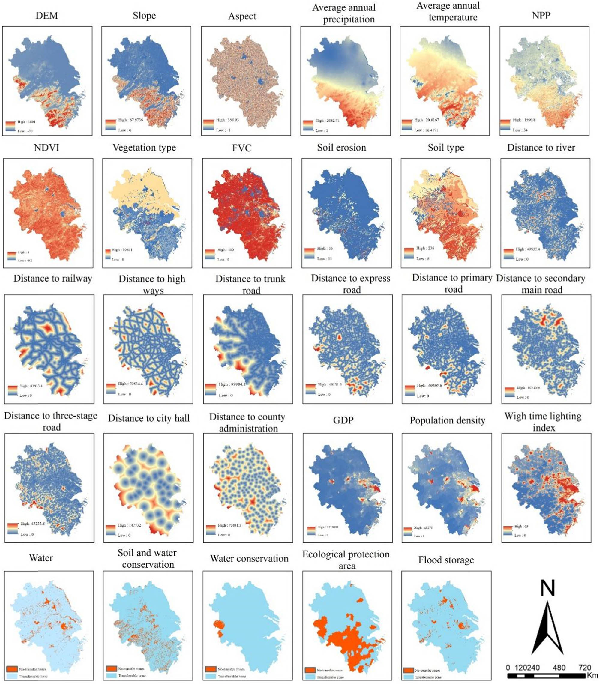
Spatial distribution of drivers and constraints.
3 Methods
3.1 Theoretical framework and Scenario design
Figure 3 illustrates the research framework of this study, encompassing LUCC prediction, CS estimation, gradient zone delineation, driving force characteristic analysis, and heterogeneity testing. First, the PLUS model was employed to simulate LUCC under various scenarios in the YRD region for 2030 and 2060, constructing an LUCC dataset spanning from 2000 to 2060 to provide data support for the spatiotemporal analysis of long-term CS variations. Second, the InVEST model was applied to evaluate CS under different development periods and scenarios from 2000 to 2060, generating data to identify the driving factors influencing CS changes. Based on socioeconomic and critical ecological data from the YRD region, the TOPSIS method was utilized to delineate economic and ecological gradients. For all the study areas and gradient zones, the CatBoost-SHAP and OPGD models were respectively utilized to construct the relationship analysis framework between natural factors, socio-economic factors, and CS. The CS prediction data and driving factor data of PLUS-InVEST were input to quantify the driving force of CS changes and reveal the driving force characteristics of CS. Finally, the WA model was applied to analyze regional gradient heterogeneity in the relationships among urban economy, ecology, and CS across different latitudinal and longitudinal zones.
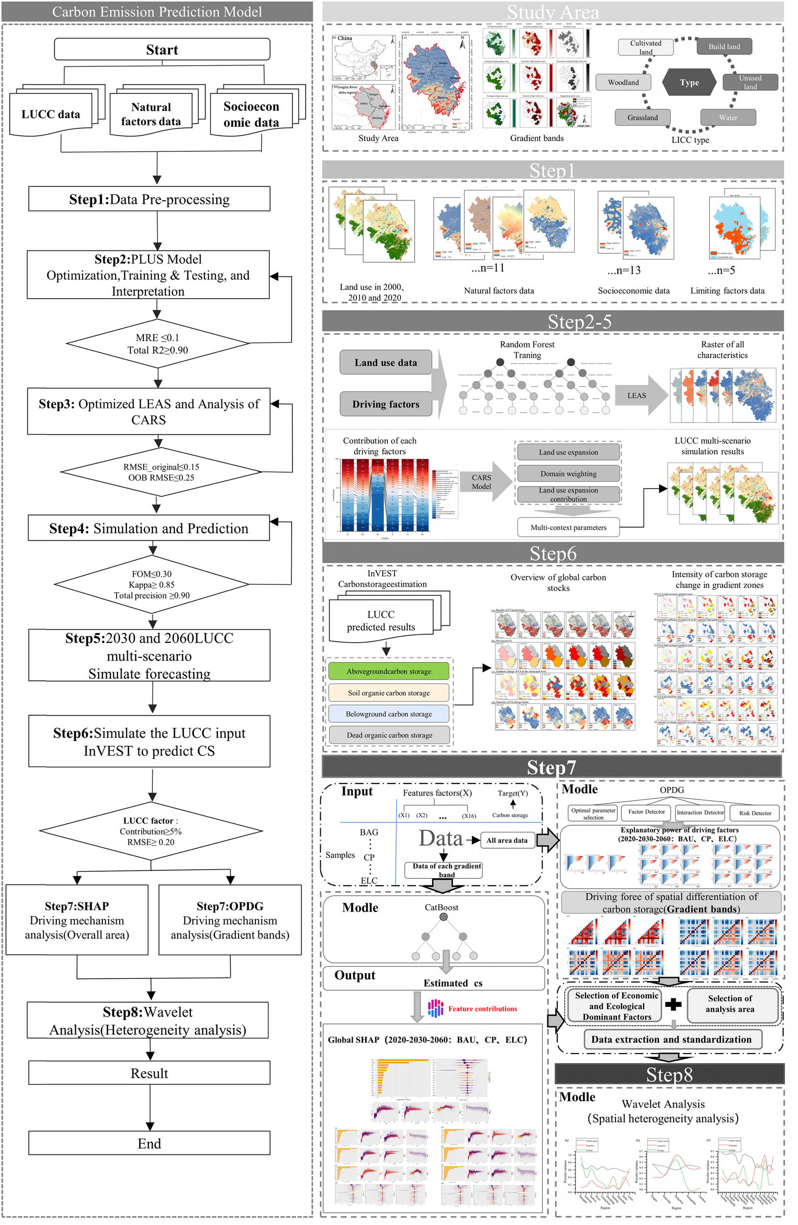
Research framework.
3.2 PLUS-InVEST models chain
3.2.1 Scenario design based on PLUS
The Patch generation land simulation (PLUS) model, developed by Liang Xun et al. at China University of Geosciences, integrates ecological conservation and planned development zones to simulate LUCC [38]. This study applied PLUS to predict LUCC in the YRD for 2030 and 2060. Using the Land Expansion Analysis Strategy (LEAS), development probabilities for LUCC types were derived via the Random Forest algorithm. The model was calibrated using 2000–2020 LUCC data, incorporating transition probability matrices, neighborhood weights, and multi-seed CARS simulations (Table 2) [39,40]. Validation achieved high accuracy (Kappa = 0.9267, FoM = 0.2586), confirming model reliability. This study selected three scenarios: BAU, CP, and ecological protection (ELC).
Multi-scenario land transfer matrix
| LUCC | BAU | CP | ELC | |||||||||||||||
|---|---|---|---|---|---|---|---|---|---|---|---|---|---|---|---|---|---|---|
| CL | WL | GL | W | UL | BL | CL | WL | GL | W | UL | BL | CL | WL | GL | W | UL | BL | |
| CL | 1 | 1 | 1 | 1 | 1 | 1 | 1 | 0 | 0 | 0 | 0 | 0 | 1 | 1 | 1 | 1 | 0 | 1 |
| WL | 1 | 1 | 1 | 0 | 0 | 1 | 1 | 1 | 1 | 0 | 1 | 1 | 0 | 1 | 0 | 0 | 0 | 0 |
| GL | 1 | 1 | 1 | 1 | 1 | 1 | 1 | 1 | 1 | 1 | 1 | 1 | 0 | 1 | 1 | 1 | 0 | 0 |
| W | 1 | 0 | 1 | 1 | 1 | 1 | 1 | 0 | 1 | 1 | 1 | 1 | 1 | 1 | 0 | 1 | 0 | 0 |
| UL | 1 | 0 | 1 | 1 | 1 | 1 | 1 | 1 | 1 | 1 | 1 | 1 | 1 | 0 | 1 | 1 | 1 | 1 |
| BL | 1 | 0 | 1 | 1 | 1 | 1 | 0 | 0 | 0 | 0 | 0 | 1 | 1 | 0 | 1 | 1 | 0 | 1 |
Note: CL (cultivated land), WL (woodland), GL (grassland), W(Water), UL (unused land), BL (building land).
Scenario 1 (BAU): Changes occur in accordance with natural principles, the historical progress of the area, and prevailing market dynamics without the introduction of any targeted policy measures. Based on LUCC alteration trends from 2000 to 2020, factors like LUCC transition likelihoods and neighborhood influence weights were preserved.
Scenario 2 (CP): Within the LUCC change categories in the YRD region, CL accounts for a significant portion. The CP scenario aims to either sustain or rehabilitate agricultural land to enhance food security and foster the vitality of agroecosystems. It limits non-agricultural development from encroaching upon CL for its protection, thereby decreasing the conversion of CL into other LUCC categories.
Scenario 3 (ELC): The ecological service framework emphasizes ecological protection and rehabilitation, ensuring the health of ecosystems and biodiversity by refining the arrangement of ecological spatial resources. Factors related to ecological conservation and restoration are incorporated as limitations to protect ecological service areas. Essential ecological conservation spaces, including forests, grasslands, and aquatic environments, are classified as non-conversion zones.
3.2.2 InVEST model
Developed by the Natural Capital Project in the United States, the Integrated Valuation of Ecosystem Services and Trade-offs (InVEST) model enables the quantitative assessment of ecosystem services with spatial visualization capabilities [41]. The InVEST model’s CS module divides ecosystem CS into four fundamental carbon pools: aboveground biomass carbon, belowground biomass carbon, soil carbon, and dead organic matter carbon [42]. The calculation formula is as follows:
where
where
Data on carbon density, essential for the CS and sequestration module within the InVEST model, were thoroughly cited from the “2010 China Terrestrial Ecosystem Carbon Density Dataset” as well as pertinent research documents. Given the variability in carbon density values reported by various researchers’ studies indicate that differences in carbon density among land types within the same climate zone are generally minimal. Therefore, drawing on previous research, data from the southeastern coast and the YRD region were utilized as references [43,44]. The soil carbon density was calculated by averaging the findings of earlier investigations, with adjustments made to the carbon density values from studies in adjacent regions based on the annual average precipitation and temperature of the study area [15,45]. The core formula is as follows (4)–(10):
where
Carbon density of different land use types in the YRD urban agglomeration/t·hm-2
| LUCC type | C_above | C_below | C_soil | C_dead |
|---|---|---|---|---|
| CL | 18.873 | 12.458 | 86.635 | 2.411 |
| WL | 36.339 | 7.368 | 121.572 | 3.341 |
| GL | 17.464 | 20.849 | 104.701 | 2.879 |
| W | 0.675 | 0 | 81.962 | 0 |
| UL | 24.295 | 4.848 | 80.719 | 2.252 |
| CL | 16.353 | 3.231 | 72.925 | 0 |
Note: CL (cultivated land), WL (woodland), GL (grassland), W (water), UL (unused land), BL (built land).
3.3 TOPSIS: Gradient band division
TOPSIS is a method for analyzing multi-attribute decisions, first introduced by C.L. Huang and Y.K. Oon in 1981. Fausto and Pan et al. ranked the alternatives by comparing their proximity to the positive ideal solution and the negative ideal solution, ultimately selecting the alternative closest to the positive ideal solution and farthest from the negative ideal solution as the optimal solution [46,47]. The formulas are as follows:
where
3.4 Gradient-multiscale coupling analysis
3.4.1 CatBoost-SHAP coupling: CS-driven analysis
3.4.1.1 CatBoost
As shown in Figure 4, we compared the performance of mainstream machine learning models including CatBoost, k-nearest neighbors (KNN), support vector machine (SVM), extreme gradient boosting (XGBoost), multilayer perceptron (MLP), and random survival forest (RSF). The CatBoost algorithm demonstrated significant advantages. A CatBoost model with an R 2 ranging from 0.8 to 1 in both training and testing results was selected. CatBoost is a highly efficient machine learning algorithm particularly well-suited for analyzing datasets with categorical features. It effectively manages high-dimensional spaces and complex nonlinear interactions among features [53], demonstrating significant strengths in capturing intricate nonlinear relationships among variables while exhibiting considerable resistance to overfitting [54]. In research related to LUCC and CS, CatBoost can be employed to develop models that connect driving factors to CS, as well as to evaluate the driving forces behind changes in CS across various scenarios [6,40]. This study integrates CatBoost with SHAP to investigate the relationship between the driving factors of CS and the variations in CS across multiple scenarios within the YRD region.
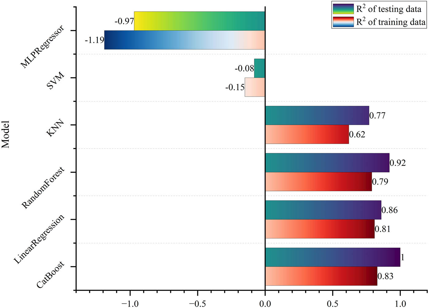
Evaluate the R 2 of the machine learning model.
3.4.1.2 SHAP
SHAP is a method for interpreting the output of any machine learning model [55], derived from the concept of Shapley values in game theory [56]. The SHAP method evaluates the importance of each feature by calculating the sum of its marginal contributions to the model output across all possible permutations. This concept has been applied in machine learning to assess how each feature contributes to the model’s predictions. The formula for calculating SHAP values is as follows:
where
where
3.4.2 OPGD
According to OPGD, the model’s accuracy and interpretability were enhanced through the incorporation of parameter optimization mechanisms and multifactor analysis, which revealed the spatial relationships among various variables. In this research, four detectors – Factor Detector, Optimal Parameter Detector, Interaction Detector, and Risk Detector – were selected from the GD package in R. These detectors were employed to discretize the driving factors of CS and conduct optimal parameter analysis, aiming to identify the most effective categories of driving factors. A higher q value (0–1) indicates an improved explanatory capacity for the spatial variability of CS, as illustrated in the following formulas:
where
3.5 Spatial heterogeneity analysis
Wavelet Variance (WV) is a powerful tool for analyzing the intensity of variation across spatial scales, particularly in identifying spatial hierarchies and characteristic scales. By decomposing data into different scales, it can reveal multi-scale patterns hidden within the data [58,59]. In this study, based on the extensive geographical span of the YRD region, samples were collected across three latitudinal belts and one longitudinal belt, spanning various gradient zones. Socioeconomic, ecological, and CS data were extracted from these sample belts. The WV method was applied to discretize the correlated data, and the root mean square error of each sample was calculated to examine the heterogeneity of spatial variations in CS across gradient zones in the YRD. This process was executed using the wavelet analyzer toolkit in MATLAB R2023b, computing wavelet coefficients, modes, mode squares, and variances for the combinations of socioeconomic, ecological, and CS data across different cross-sections. The WV formula is given as follows:
where
where
4 Results and analysis
4.1 Differentiation of gradient bands
This study applied the TOPSIS method to delineate ecological and economic gradient zones in the YRD using socioeconomic-ecological data, with integrated gradient zones derived from combined coefficients ( Figure 5). Ecological gradients exhibited significant disparity (high: 0.632; low: 0.011), reflecting spatial differentiation in ecological sensitivity and conservation intensity. High ecological gradients clustered in critical service zones, notably western Zhejiang and Anhui. Economic gradients showed extreme polarization (high: 0.960; low: 0.004), dominated by urban cores like Shanghai and provincial capitals, with peripheral areas displaying gradient decline. Transition zones, balancing economic (0.190–0.275) and ecological coefficients, functioned as buffer areas between development and conservation. Special zones (e.g., Hangzhou, Suzhou, Lianyungang) demonstrated dual high ecological-economic gradients, representing sustainable synergy hotspots.
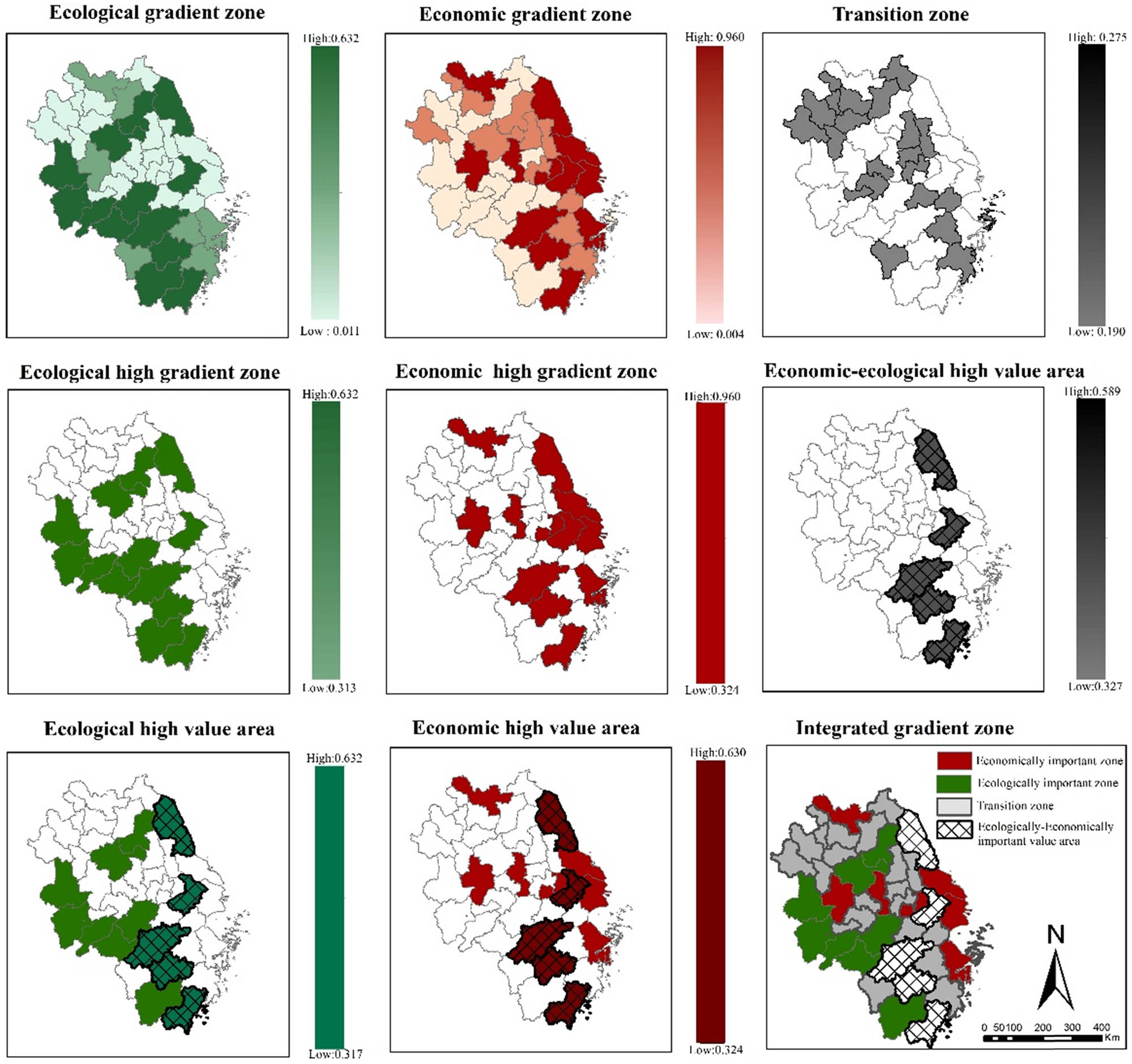
Gradient band partition results.
4.2 Evolution and prediction results of LUCC under the gradient pattern
4.2.1 Gradient zone LUCC transition differentiation from 2000 to 2020
The comparison of the simulation results with the real data of 2020 shows that the error between the simulation data and the real data is less than 10%, and mostly within 5%. The accuracy of the simulation results is relatively high (Table 4). From 2000 to 2020, CL and WL dominated LUCC patterns in the YRD (Figure 6). Combined, these land types accounted for 93.50, 93.70, and 94.12% of total LUCC area in 2000, 2010, and 2020, respectively. CL remained predominant but exhibited a persistent decline, decreasing from 56.08% (2000) to 52.99% (2020). WL, the second-largest category, showed a “decline-recovery” trend, dropping from 30.56% (2000) to 28.65% (2020). Built-up land expanded continuously, with a cumulative increase of 5.83% by 2020, while other land types diminished. Significant LUCC conversions occurred during this period, accompanied by notable shifts in spatial distribution (Figure 7). Among them, the one with the largest expansion is BL, and the one with the largest reduction is CL. BL and CL are concentrated in the eastern coastal and inland economic high-gradient zones (HGZ) of the YRD region. In this area, the transformation of CL and built land has dominated, resulting in the fragmentation of ecological service land in the northern part of the YRD region and within the economic HGZ. The intensity of change is large in Jiangsu Province and Anhui Province, among which Suzhou, Wuxi, Nanjing, Xuzhou, and Hefei are the most significant. WL and GL are mainly distributed in the mountainous areas in the southwest of Anhui Province and Zhejiang Province. In Anhui province, they are concentrated in Lu’an, Anqing, Chizhou, Huangshan, and Xuancheng. In Zhejiang province, they are mainly concentrated in Hangzhou, Quzhou, Jinhua, Lishui, Taizhou, and Wenzhou. 95% of them are within the ecological HGZ, and the variation range of LUCC in this area is smaller compared with that in the economic HGZ. It prompts the focus of important ecological land, such as WL and GL, to shift southward. Zhejiang Province and the southern part of Anhui Province are the ecological core areas of the entire YRD region, and high-CS land is fully concentrated in the ecological high-gradient area in the southwest.
LUCC prediction accuracy (km2)
| Year | CL | WL | GL | W | UL | CL |
|---|---|---|---|---|---|---|
| 2020 True (km2) | 182326.229 | 105014.040 | 56.7486 | 22167.93 | 4.3497 | 43566.547 |
| 2020 Forecast (km2) | 176437.092 | 103596.348 | 52.748 | 21112.733 | 3.972 | 40669.371 |
| Error (%) | 3.23 | −1.35 | 7.05 | 4.76 | −8.69 | 6.65 |
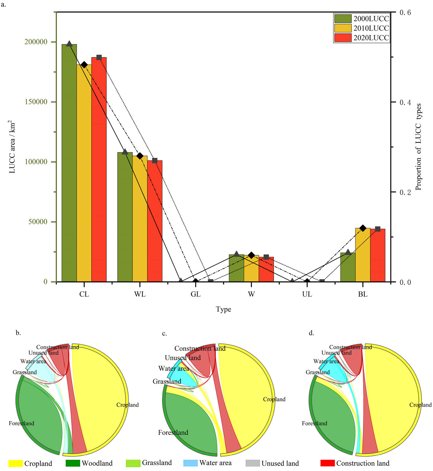
Overview of land use structure change and transfer from 2000 to 2020; (a) 2000–2020 LUCC utilization overview, (b), 2000–2010, (c) 2010–2020, and (d) 2000–2020. CL (cultivated land), WL (woodland), GL (grassland), W (water), UL (unused land), BL (built land).
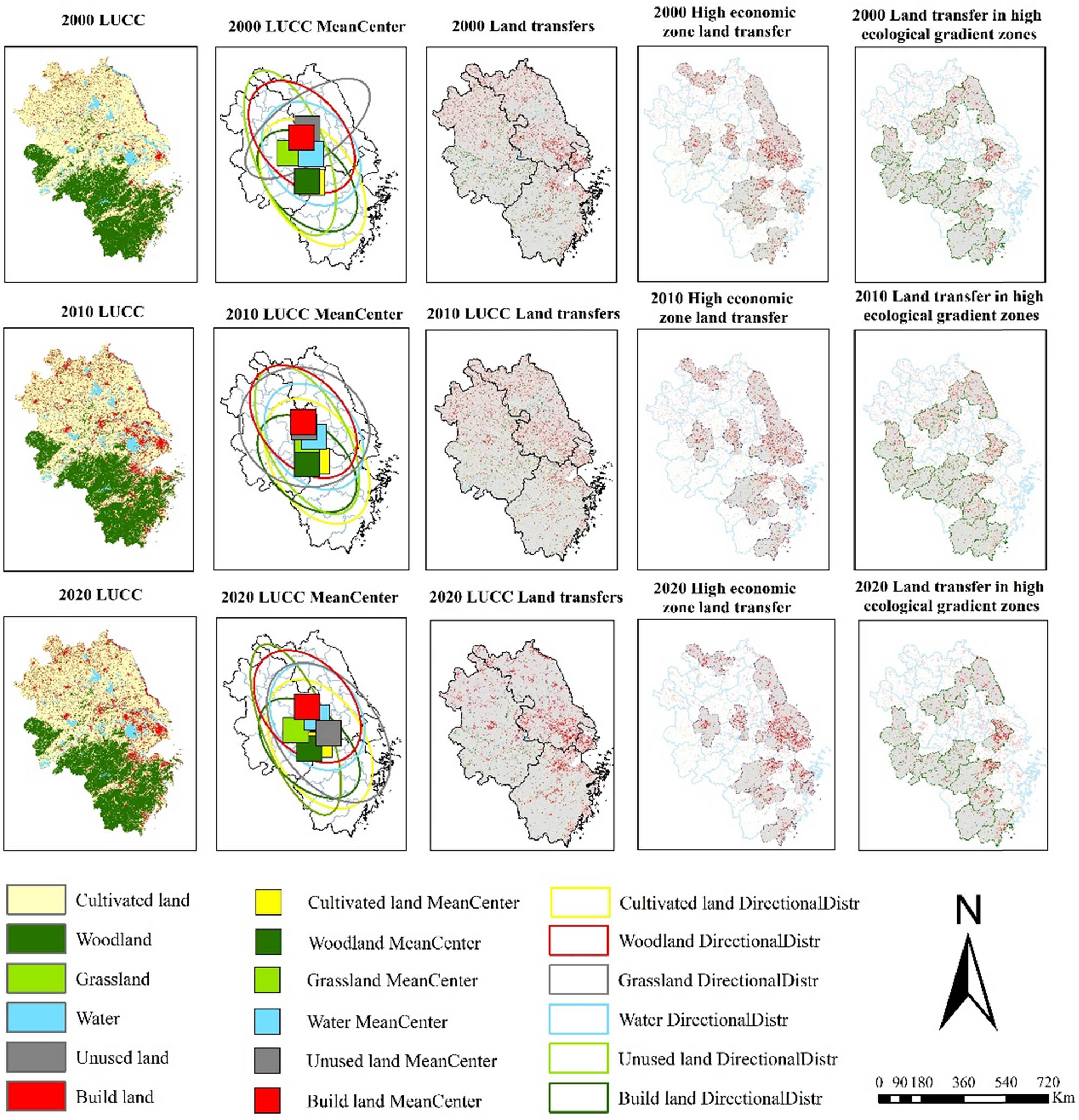
Spatial variation characteristics of LUCC.
4.2.2 LUCC multi-scenario simulation comparison
The PLUS model simulated LUCC in the YRD under three scenarios (BAU, CP, ELC) for 2030 and 2060 (Figure 8). The most intensive changes occurred in high-economic-gradient zones centered on Shanghai and provincial capitals, characterized by urban agglomerations, while minimal changes persisted in high-ecological-gradient zones (western Anhui and Zhejiang), which retained over 80% of ecological carbon sinks.
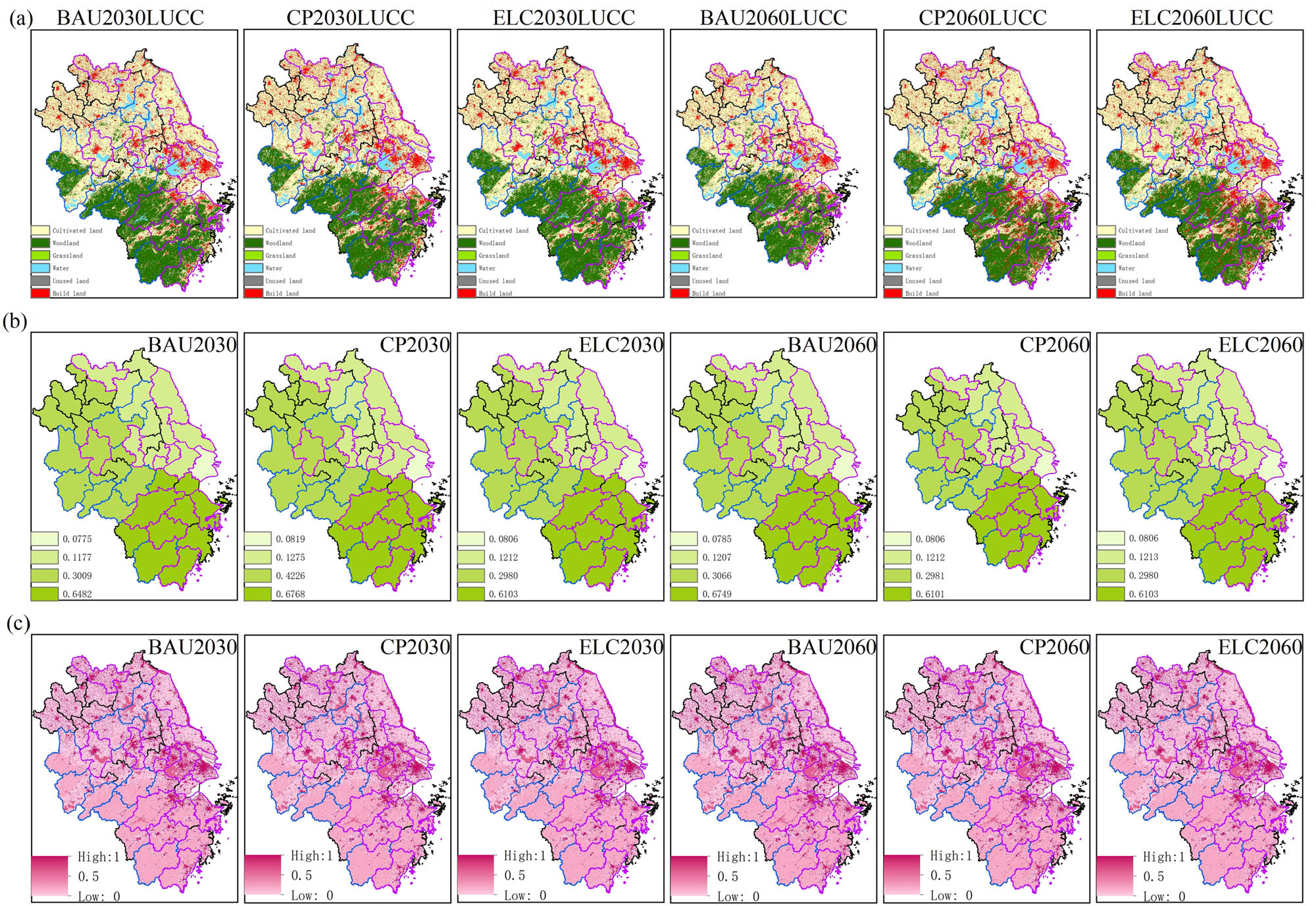
Spatial intensity characteristics of multi-scenario LUCC in 2030 and 2060. (a) LUCC spatial distribution map under multi-scenario development model. (b) Percentage of ecological land by providence (2030–2060), (c) LUCC expansion potential (2030–2060).
Significant variations in LUCC were observed in 2030 and 2060 under different scenarios (Figure 9). Among the three scenarios, the most pronounced changes occurred in CL, WL, and BL. Under the BAU scenario, compared with 2030 and 2020, the BL in 2060 increased by 17.06% and 18.98%, respectively, with a cumulative increase of 1.01 × 10⁴ km2. Zhejiang Province and Anhui Province had the greatest changes. The growth intensity of BL in Jiaxing, Hangzhou, Shaoxing, Ningbo, Jinhua, Taizhou, Wenzhou, Anqing, Fuyang, Bozhou, Huaibei, Suzhou, and Bengbu is significant. The area of WL decreased by 2.96 and 4.53%, respectively, with a cumulative reduction of 4.82 × 10³ km2. The intensity of the decline in the area of WL was the greatest in Hangzhou, Shaoxing, Ningbo, Jinhua, and Wenzhou of Zhejiang Province. The area of CL decreased by 6.01 and 4.17%, respectively, with a cumulative reduction of 4.22 × 10³ km2. The reduction areas were concentrated in Anhui Province and Jiangsu Province, which occupy approximately 90% of the CL in the YRD. The rapid expansion of cities occupied a large amount of CL. Under the CP scenario, the areas with a relatively large intensity of Land use change are concentrated in the underdeveloped central and western regions of Zhejiang Province and Anhui Province. The UL changes most significantly, decreasing by 49.19 and 46.00%, respectively in 2030 and 2060. BL followed, increasing by 11.34 and 14.77%, with a cumulative growth of 6.51 × 10⁴ km2. CL remained relatively stable from 2030 to 2060. In the ELC scenario, UL decreased sharply by 73.78 and 95.18% in 2030 and 2060, respectively, while BL expanded by 6.11 and 11.09%. Ecological service lands such as WL, GL, and W experienced minor fluctuations, showing a slow upward trend.
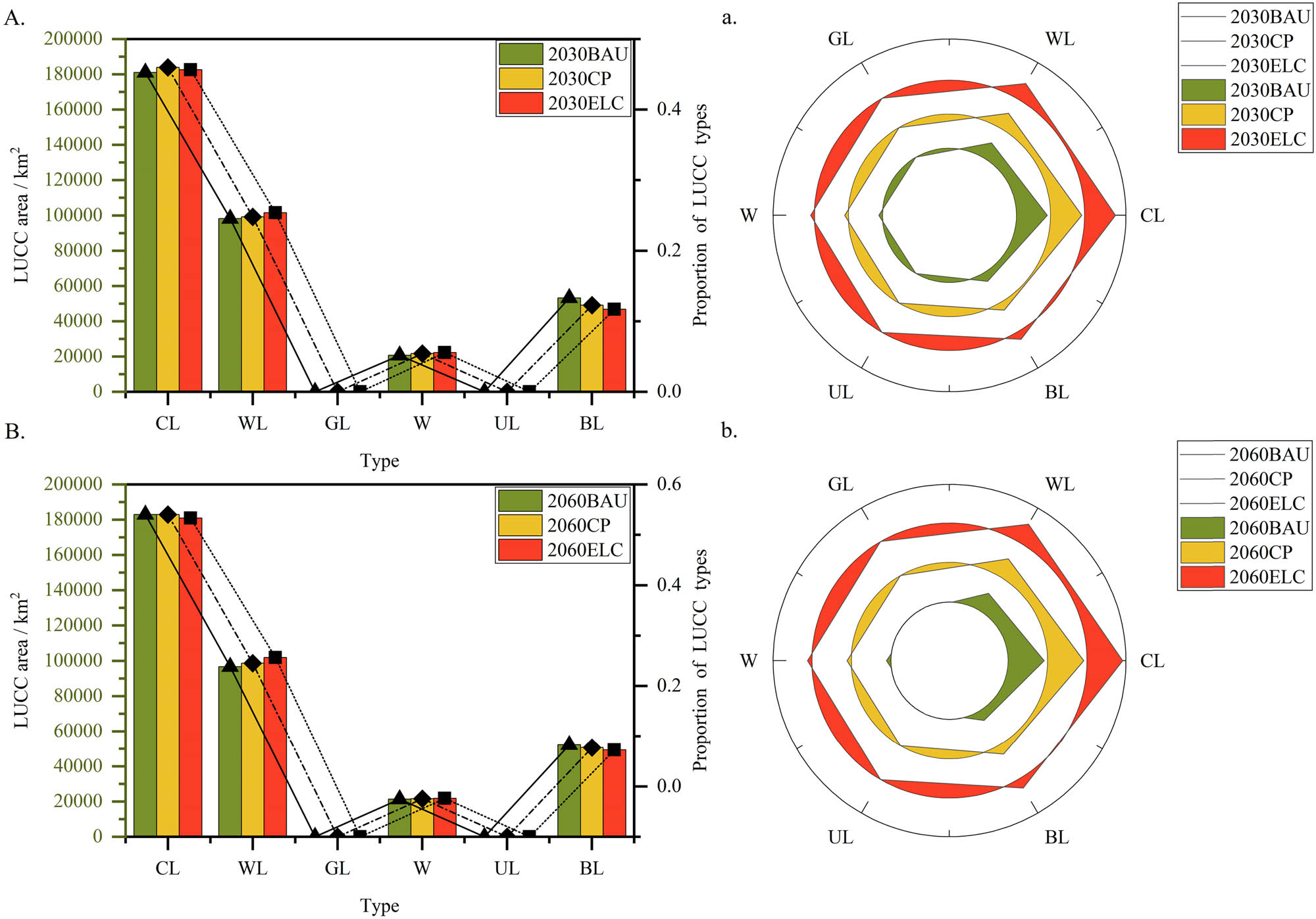
Structure and variation characteristics of 2030 and 2060 LUCC, CL, WL, GL, W, UL, and BL. (A) 2030, (a) 2030), (B) 2060, (b) 2060.
4.3 Spatiotemporal evolution and threshold of gradient CS
4.3.1 Multi-scenario CS forecasting
The CS from 2000 to 2060 was assessed using the InVEST model. From 2000 to 2020, CS decreased from 4618.95 × 106 t in 2000 to 4592.31 × 106 t in 2010 and further to 4552.63 × 106 t in 2020, with a cumulative decline of 66.32 × 10⁶ t over the 20 years. During this period, significant changes in CS were observed for CL, WL, and BL land. Specifically, CS in CL and WL decreased by 189.04 × 10⁶ t and 49.49 × 10⁶ t, respectively, while CS in BL land increased by 178.98 × 10⁶ t. The remaining three land-use types also exhibited declining CS trends, albeit with smaller magnitudes of change (Table 5).
CS by land type (106 t)
| Type | Year and scene | ||||||||
|---|---|---|---|---|---|---|---|---|---|
| 2000 | 2010 | 2020 | 2030BAU | 2030CP | 2030ELC | 2060BAU | 2060CP | 2060ELC | |
| CL | 2383.83 | 2237.00 | 2194.79 | 2183.52 | 2187.63 | 2182.52 | 2180.87 | 2185.87 | 2181.87 |
| WL | 1820.24 | 1840.29 | 1770.75 | 1735.68 | 1751.68 | 1781.28 | 1715.30 | 1767.52 | 1801.41 |
| GL | 2.86 | 2.49 | 0.83 | 0.61 | 0.61 | 0.80 | 0.74 | 0.81 | 0.91 |
| W | 187.76 | 200.78 | 183.19 | 161.08 | 171.08 | 179.57 | 169.40 | 176.70 | 182.58 |
| UL | 0.22 | 0.08 | 0.05 | 0.04 | 0.02 | 0.02 | 0.02 | 0.01 | 0.01 |
| BL | 224.05 | 311.66 | 403.03 | 464.15 | 457.97 | 451.40 | 494.97 | 483.02 | 481.21 |
| SUM | 4618.95 | 4592.31 | 4552.63 | 4545.08 | 4568.99 | 4595.59 | 4561.3 | 4613.93 | 4647.99 |
Note: CL (cultivated land), WL (woodland), GL (grassland), W (water), UL (unused land), BL (built land).
By 2030, the CS values are projected to be 4545.08 × 106 t, 4568.99 × 106 t, and 4595.59 × 106 t, respectively, showing an overall declining trend, though the decrease is relatively modest compared to the period from 2000 to 2020. The CS for built-up land continues to rise, with values of 464.15 × 10⁶ t, 457.97 × 10⁶ t, and 451.40 × 10⁶ t under the three development scenarios. The BAU scenario exhibits the largest increase in CS, while the CP and ELC scenarios show similar increments, with the ELC scenario having the smallest CS. From 2020 to 2030, the WL CS values under the three scenarios are 1735.68 × 106 t, 1751.68 × 106 t, and 1781.28 × 106 t, respectively. The CS under BAU and CP scenarios decreases slightly, whereas the ELC scenario shows a minor increase of 10.53 × 10⁶ t. Changes in CS for other land-use types are relatively minor Table 5). By 2060, the CS values under BAU, CP, and ELC scenarios are projected to be 4561.3 × 106 t, 4613.93 × 106 t, and 4647.99 × 106 t, respectively. Under CP and ELC scenarios, the CS in 2060 exceeds that of 2020 and 2030, with increases of 61.30 × 10⁶ t and 95.36 × 10⁶ t compared to 2020. In contrast, the BAU scenario shows a declining trend in CS relative to 2020 and 2030. Spatially, the CS distribution in the YRD region exhibits significant north-south disparities. High-CS areas are concentrated in Zhejiang and Anhui, while Jiangsu and Shanghai have relatively lower CS values (Figure 10). Regions with drastic CS changes are primarily located in Zhejiang, which is characterized by mountainous terrain and dense ecological land use. The rapid economic growth in Zhejiang makes its ecological CS more sensitive to impacts. In contrast, ecological zones in Jiangsu and Anhui are more dispersed and smaller in scale, resulting in lower sensitivity to economic development and urban expansion, with correspondingly smaller changes in CS intensity.
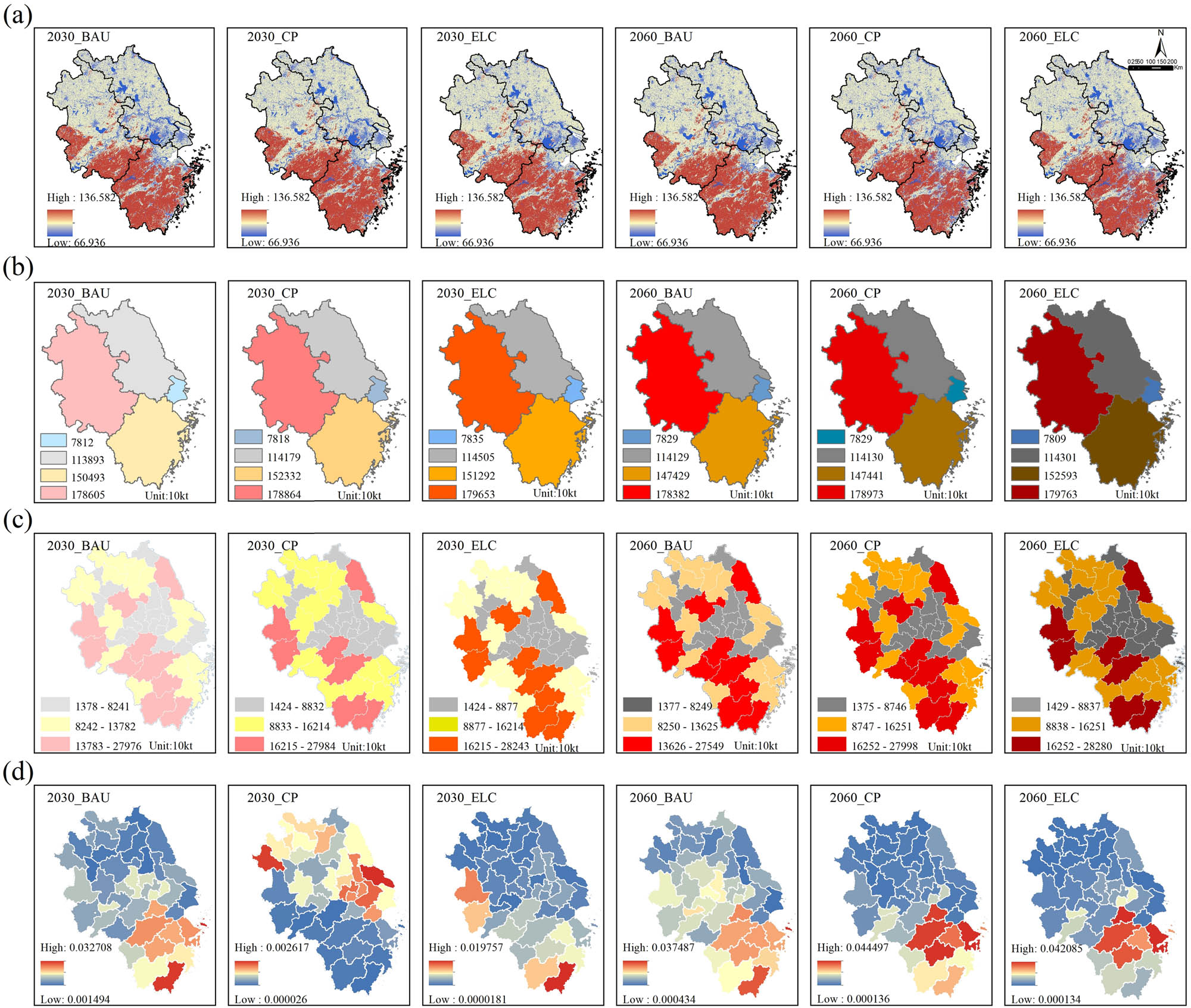
Spatiotemporal characteristics of multi-scale CS. (a) Results of CS projections, (b) Provincial CS, (c) Gradient change in CS at the municipal level, and (d) CS change intensity.
4.3.2 CS gradient variation characteristics and thresholds
From 2000 to 2060, the CS in the high ecological gradient zone remained stable at 2246.98 × 106 t to 2316.44 × 106 t, while that in the high economic gradient zone ranged from 1529.47 × 106 t to 1574.96 × 106 t. The CS in the high ecological gradient zone consistently maintained a level 1.5 times higher than that in the high economic gradient zone. The CS in the transitional zone fell between these two regions, ranging from 1576.81 × 106 t to 1614.98 × 106 t, still showing a significant gap compared to the high ecological gradient zone, with relatively minor fluctuations (Table 6).
CS in each gradient zone (106 t)
| Type | Year and scene | ||||||||
|---|---|---|---|---|---|---|---|---|---|
| 2000 | 2010 | 2020 | 2030BAU | 2030CP | 2030ELC | 2060BAU | 2060CP | 2060ELC | |
| Intensity coefficient of CS | 1574.96 | 1558.45 | 1543.73 | 1529.47 | 1538.92 | 1546.23 | 1543.76 | 1553.05 | 1566.14 |
| Ecological HGZ | 2285.94 | 2283.95 | 2264.59 | 2246.98 | 2251.37 | 2263.88 | 2268.84 | 2305.42 | 2316.44 |
| Transition Z | 1614.98 | 1600.57 | 1586.17 | 1576.81 | 1584.75 | 1594.55 | 1587.58 | 1599.69 | 1611.72 |
Note: CL (cultivated land), WL (woodland), GL (grassland), W (water), UL (unused land), BL (built land), HGZ (high-gradient zone).
From 2000 to 2020, the cumulative CS in the high ecological gradient zone decreased by 21.35 × 10⁶ t. Under the BAU scenario from 2020 to 2030, CS continued to decline, reaching a minimum value of 2246.98 × 106 t. By 2060, the CS values in the high ecological gradient zone under the BAU, CP, and ELC scenarios were 2268.84 × 106 t, 2305.42 × 106 t, and 2316.44 × 106 t, respectively. Within the high ecological gradient zone, the extremely high CS values ranged from 8,242 × 104 t to 13,411 × 104 t. This region is an intensive ecological service area where LUCC structural changes exhibit high sensitivity to ecological CS, primarily distributed in Anhui and Zhejiang provinces. From 2000 to 2020, CS in the high economic gradient zone decreased by 31.23 × 10⁶ t. Under the BAU and CP scenarios from 2020 to 2030, CS in the high economic gradient zone continued to decline. By 2060, CS under all three scenarios showed a sustained increasing trend, peaking at 1566.14 × 106 t. The extremely high CS zones and areas with significant fluctuations were mainly concentrated in prefecture-level cities of Zhejiang and Anhui (Figure 11).
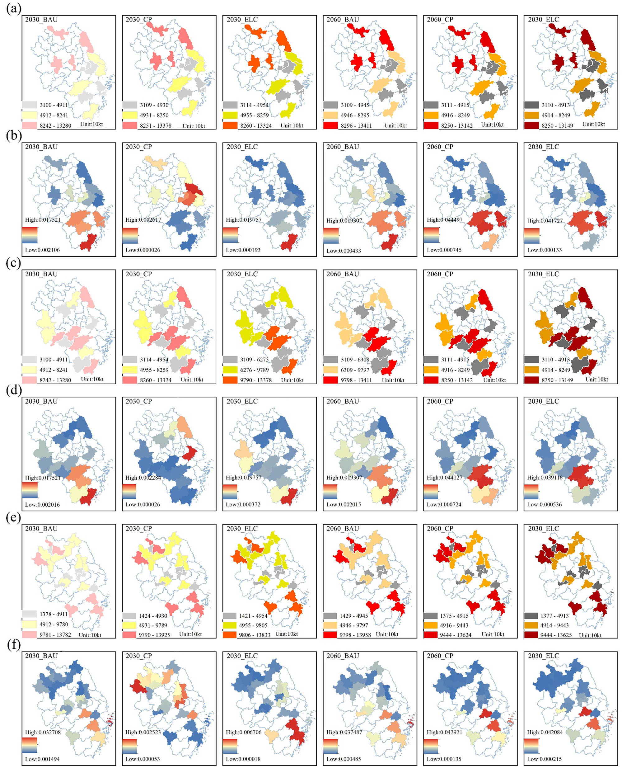
Spatial variation intensity and distribution characteristics of CS in gradient bands. (a) CS in high economic gradient zones, (b) intensity coefficient of CS in the economic HGZ, (c) CS in high ecological gradient zones, (d) intensity coefficient of CS change in ecologically HGZs, (e) CZ in the transition zone, and (f) intensity coefficient of CS change in the transition zone.
4.4 Scale feature detection of CS in gradient bands
4.4.1 CS feature detection factor selection
This study investigates spatial gradient characteristics and driving mechanisms of CS in the YRD through ecological-economic gradient analysis. CS spatiotemporal heterogeneity arises from synergistic interactions between natural and socioeconomic factors (Figure 12). Natural factors determine ecosystem CS potential, while socioeconomic drivers directly influence CS via LUCC restructuring and human activity intensity. Thirteen key drivers and three constraints were selected for CS analysis: X1 (GDP), X2 (population density), X3 (nighttime lighting index), X4 (slope), X5 (precipitation), X6 (temperature), X7 (NPP), X8 (NDVI), X9 (river proximity), X10 (DEM), X11 (FVC), X12 (vegetation type), X13 (soil type), X14 (soil-water conservation), X15 (water conservation), and X16 (ecological protection areas). This framework elucidates gradient-specific CS responses to coupled human-natural systems.
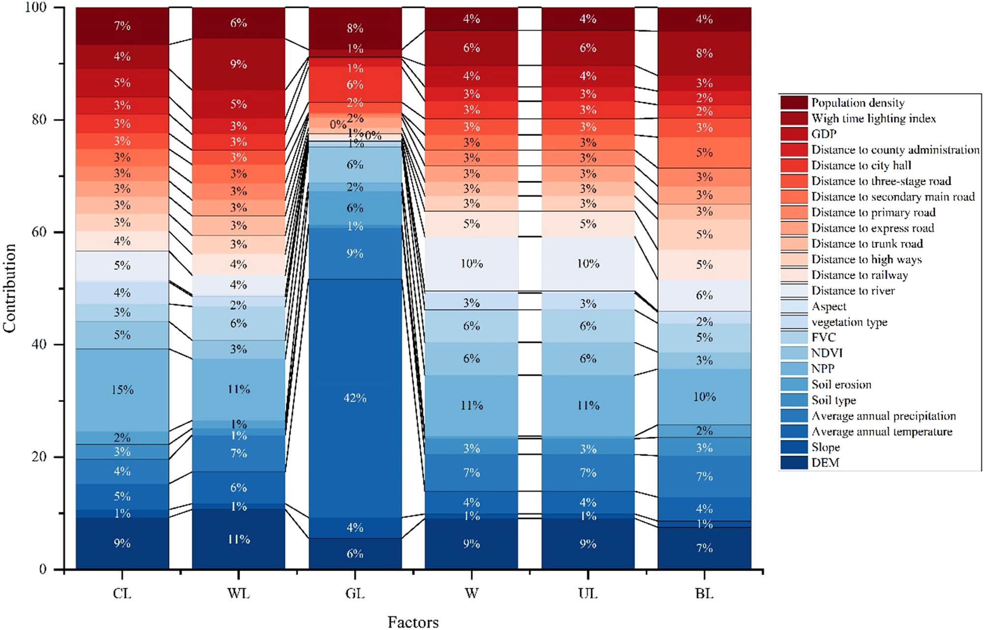
Driver contribution profile.
4.4.2 Characteristics of CS change drivers in all regions were detected
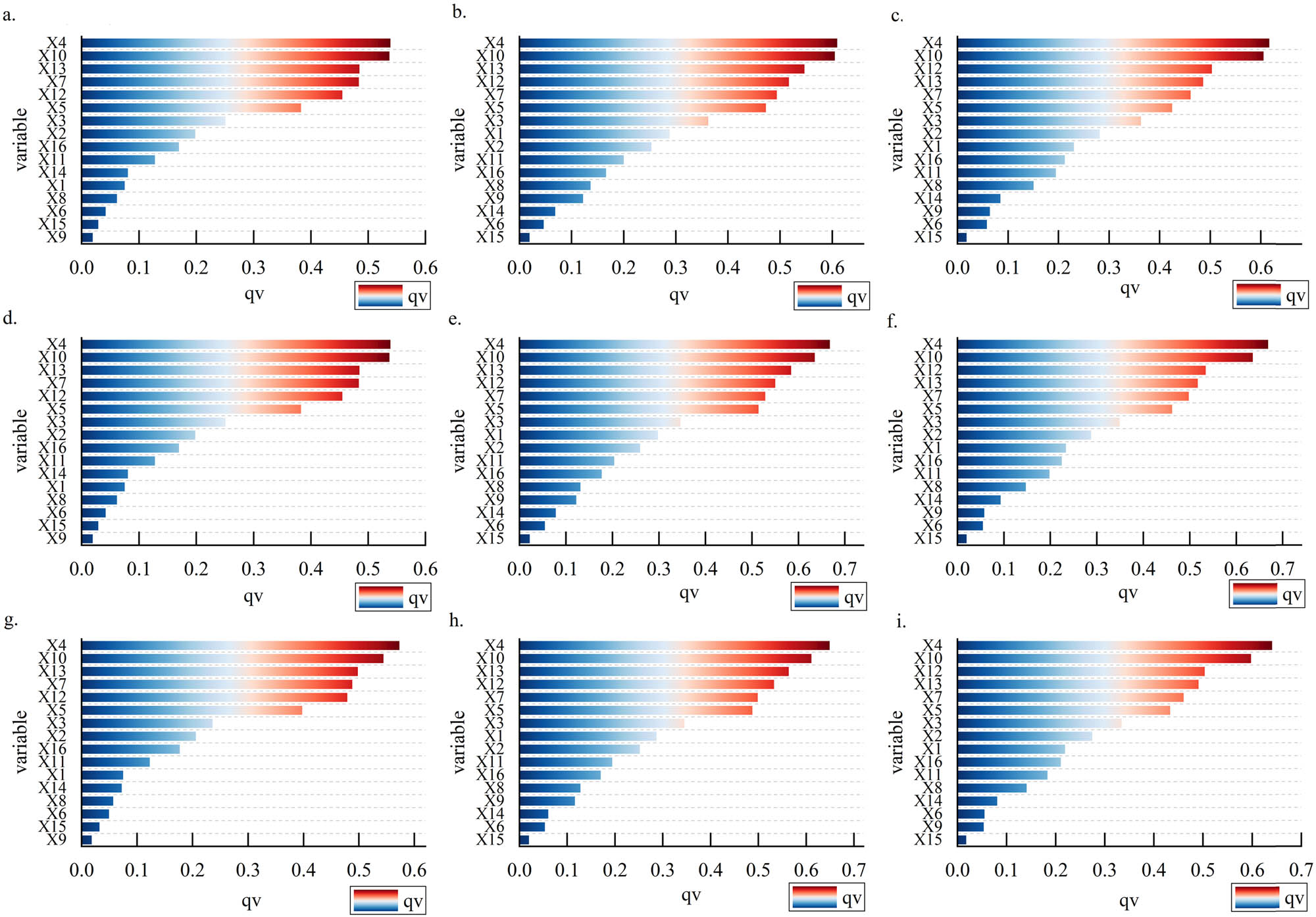
This study employed CatBoost-SHAP to assess the global and local importance of CS drivers across multiple scenarios (2020, 2030, and 2060) in the YRD (Figures 13–15). Global importance, derived from mean absolute SHAP values, identified key drivers, while local importance visualized individual SHAP values (y-axis: features; x-axis: SHAP scores; colors: feature magnitudes, yellow: high, purple: low). Positive/negative SHAP values denote factors increasing/decreasing CS predictions. Interaction mechanisms between high-impact drivers were analyzed via SHAP scatterplots, where axes represent interacting variables and point colors reflect SHAP gradients (bright: high, dark: low). This approach clarifies how terrain, vegetation, and urbanization jointly shape CS dynamics through nonlinear pathways.
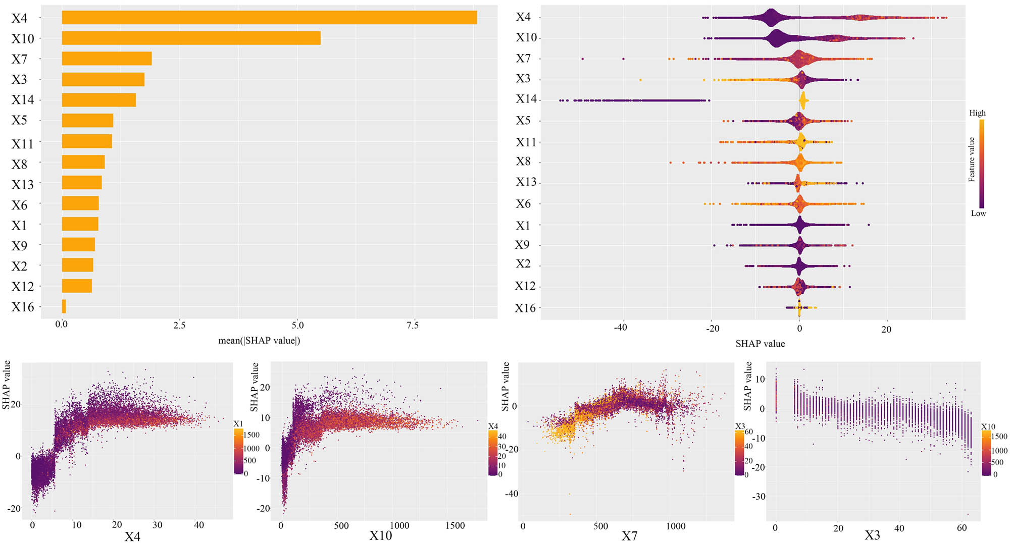
Relative importance of socioeconomic and natural ecological variables to CS in 2020.
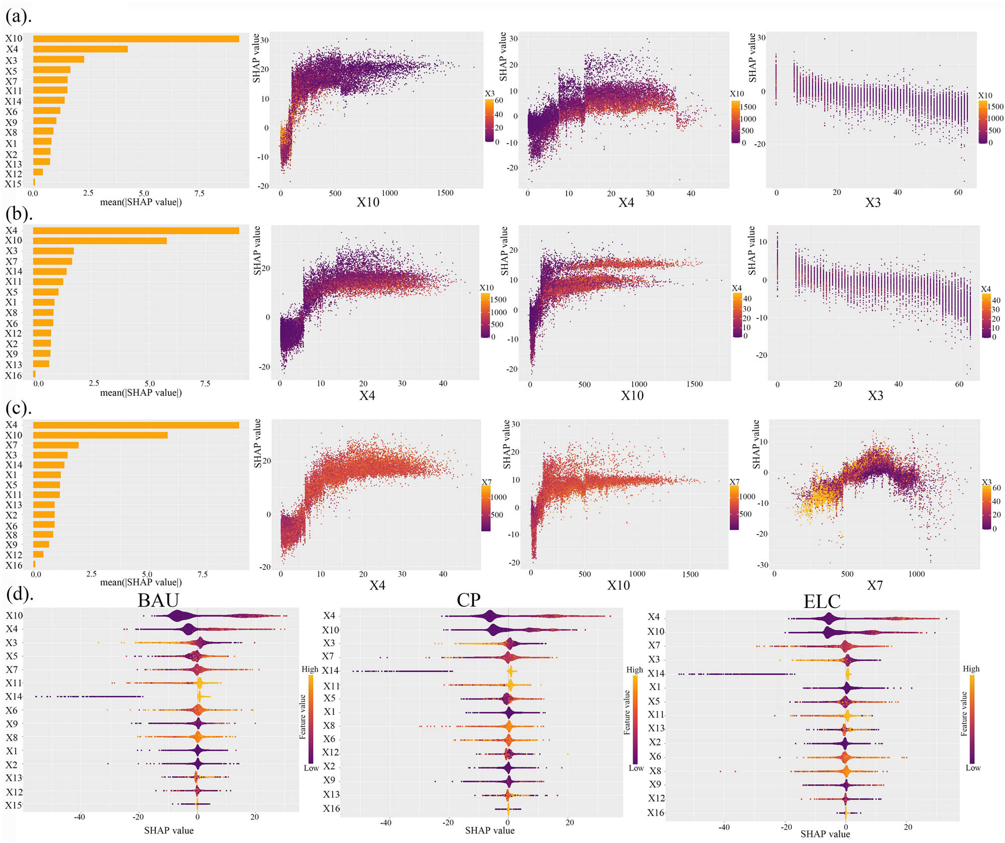
Relative importance of socioeconomic and natural ecological variables to CS in 2030. (a) 2030 BAU, (b) 2030 CP, (c) 2030 ELC, and (d) BAU.
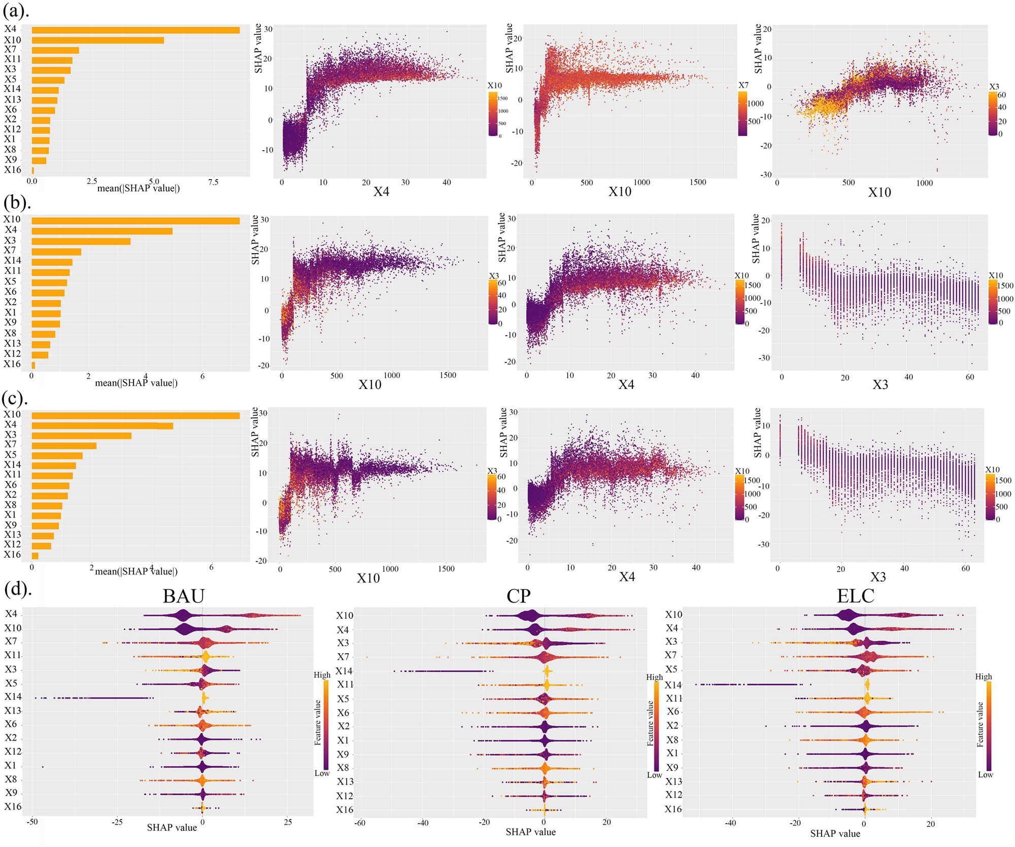
Relative importance of socioeconomic and natural ecological variables to CS in 2060. (a) 2060 BAU, (b) 2060 CP, (c) 2060 ELC, and (d) BAU.
Figure 13 demonstrates that X4 (importance: 8.7) and X10 (importance: 5.3) exhibit the strongest positive correlations with CS, consistent with linear model results. X3 significantly reduces CS, while X7 shows a moderate positive influence. Natural ecological factors dominate CS patterns due to their inherent carbon sequestration capacity, outperforming socioeconomic drivers. This is primarily because CS levels depend more on the carbon sequestration capacity of fundamental natural ecological environments, such as topographic features, natural vegetation, and soil types. The influence of the interaction of slope, DEM, NPP, and weight time lighting index on CS indicates that when X4 is 10–40 and X10 is 0–1,000, the SHAP value is 10–30. The increase in CS in the YRD region is extremely significant. The growth rate of CS is fast, and the retention quantity is large. When X3 is 20–60 and X7 is 500–1,500, the SHAP value is 10–20, which has a significant impact on CS, but the total amount of CS is relatively low, and the growth rate is slow. When X3 is 10–60 and X10 is 0–1,000, the SHAP value is 0–15, the growth of CS is relatively stable, and the total amount of CS is relatively low.
Figure 14 illustrates the importance of impact variables on CS in the YRD region by 2030. Under the BAU scenario, X10 and X4 exhibit the most significant influence on CS, with importance levels of 8.8 and 4.0, respectively. Both variables show a positive correlation with CS. In the CP and ELC scenarios, X4 and X10 remain the top two influential factors, but X4 demonstrates greater explanatory power than X10, with importance levels of 8.3 and 5.6, respectively. Across all three development modes, X14 also exerts a notable impact on CS, though its positive influence is spatially limited, primarily due to the uneven spatial distribution of soil and water conservation areas in the YRD region.
Under the BAU scenario, the influence of the interaction among X10, X4, and X3 on CS indicates that when X10 is 100–1,500 and X3 is 0–20, the SHAP value is 10–30, and CS increases significantly, but the upper limit of the total amount of CS is relatively low. In the CP scenario, when X4 is 5–60 and X10 is 0–500, the SHAP value is 0–15. The change in CS is relatively significant, and the total holding of CS is at a relatively low level. When X10 is 125–1,500 and X4 is 20–40, the SHAP value is 10–40, which has a significant impact on CS, with a high upper limit of the total amount of CS and a large overall possession of CS. In the ELC scenario, when X4 is 5–60 and X7 is 500–1,000, the SHAP value is 10–40, which has a significant impact on the growth of CS. The upper limit of CS is extremely high, and the total amount of CS is at a high level. When X10 is 250–1,500 and X7 is 500–1,000, the SHAP value is 10–30, which has a significant impact on the change in CS. The growth rate is relatively small, but it can still support the total amount of CS to remain at a relatively high level. In 2030, ecological CS will have a stronger dependence on X4 and X10. Under the CP and ELC scenarios, CS will have the strongest dependence on X4, which is better than that on X10.
Figure 15 illustrates the importance of CS impact variables in the YRD region by 2060. Under the BAU scenario, X4 and X10 exhibit the greatest influence on CS, with importance levels of 8.8 and 5.5, respectively. In both the CP and ELC scenarios, X4 and X10 remain the top two influential factors, though X10 demonstrates higher explanatory power than X4. Under the CP scenario, the importance levels of X4 and X10 are 7.5 and 5.0, respectively, while under the ELC scenario, they are 7.2 and 4.8. Under the BAU scenario, when X4 is 10–50 and X10 500–1,000, the SHAP value exceeds 10, indicating a highly significant improvement in CS. In the CP scenario, when X4 is 5–60) and X3 is 0–20, the impact on CS is relatively significant, with SHAP at 15–30. Similarly, when X4 is 10–50 and X10 0–500, the effect on CS is notable, with SHAP 15–30. Under the ELC scenario, when X10 is 100–1,500 and X3 is 0–40, the SHAP is 10–20, indicating a moderately significant influence on CS. By 2060, the enhancement of CS remains predominantly driven by X4 and X10. Under the CP and ELC development models, CS exhibits the strongest dependence on X10, surpassing that on X4.
4.4.3 Characteristic detection of CS change drivers in gradient bands
The OPGD model was employed to analyze the factors influencing CS within the economic and ecological gradient zones of the YRD region from 2020 to 2060. The detection results of driving factors at different stages are presented in Table 6.
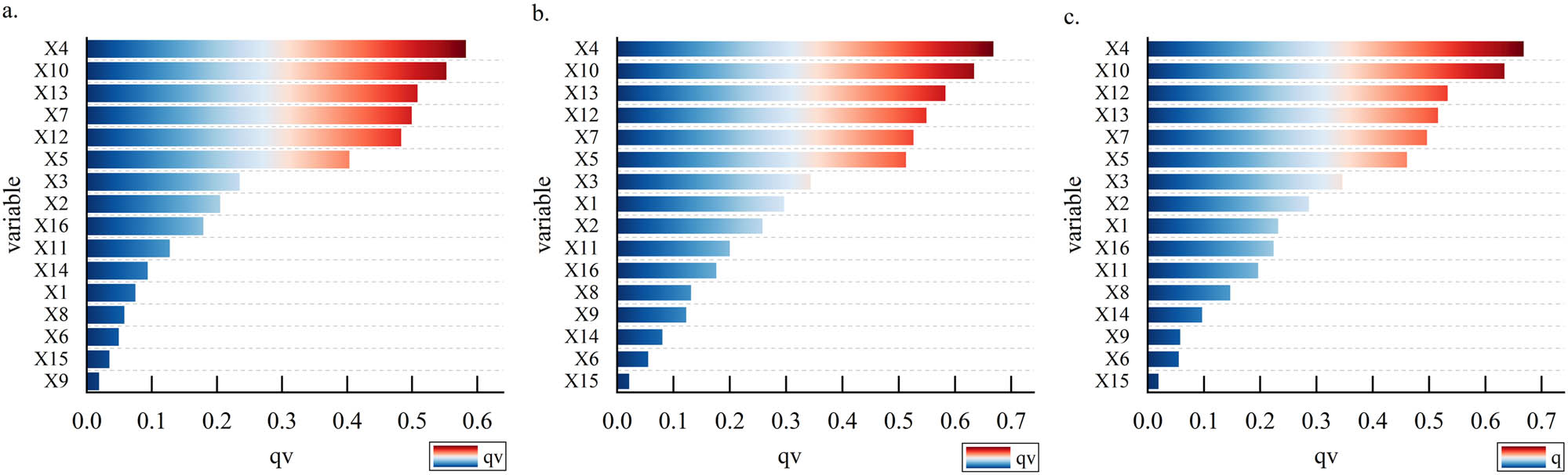
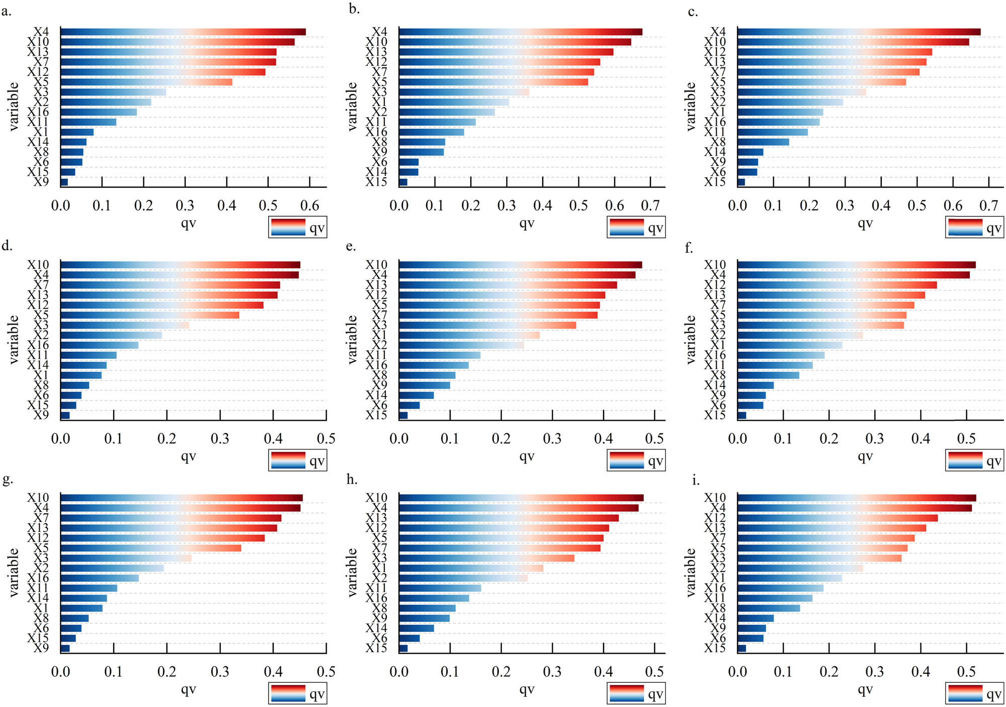
As shown in Figure 16, the factors influencing CS in the transition zone, economic HGZ, and ecological HGZ in 2020 are presented. The primary factors affecting CS in the transition zone are, in descending order, X4 (0.58), X10 (0.55), X13 (0.51), and X7 (0.50), all of which exhibit positive effects. For the economic HGZ, the main influencing factors of CS are X4 (0.67), X10 (0.63), X13 (0.58), X12 (0.55), X7 (0.53), and X5 (0.51), all demonstrating significant positive impacts. In the ecological HGZ, the dominant factors affecting CS are X4 (0.67), X10 (0.63), X12 (0.53), X13 (0.52), and X7 (0.50), all of which show significant positive influences.
The relative importance and dependence of factors affecting CS in the gradient band in 2020. (a) 2020 transition zones, (b) 2020 high economic gradient zones, and (c) high ecological gradient zones.
As shown in Figure 17, these illustrate the factors influencing CS across different gradient zones in 2030. Under the three scenarios, the primary factors affecting CS in gradient zones are X4 and X10, with their influence coefficients exceeding 0.60. In the CP and ELC scenarios, X4 and X10 reach their highest values of 0.67 and 0.63, respectively, in the high ecological-economic gradient zones. This is followed by X13, X12, and X7, which exhibit significant positive influences ranging between 0.50 and 0.60 in the high economic-ecological gradient zones, while their influence diminishes to 0.40–0.50 in the transitional zones. Under the CP and ELC scenarios, the impact of factors X4, X10, X13, X12, and X7 on CS in the high economic-ecological gradient zones is greater than that under the BAU scenario. Notably, in the CP and ELC scenarios, X13 (0.56, 0.58) exerts a stronger influence than X12 (0.55, 0.53) in the high ecological gradient zones, whereas X12 (0.53, 0.50) has a greater impact than X13 (0.52, 0.49) in the high economic gradient zones. This discrepancy arises primarily because the CP and ELC development scenarios emphasize different priorities in LUCC and ecological conservation, leading to variations in their effects on CS.
The relative importance and dependence of factors affecting CS in the gradient band in 2030. (a) 2030 (BAU) Transition zones, (b) 2030 (BAU) High economic gradient zones, (c) 2030 (BAU) High ecological gradient zones, (d) 2030 (CP) Transition zones, (e) 2030 (CP) High economic gradient zones, (f) 2030 (CP) High ecological gradient zones, (g) 2030 (ELC) Transition zones, (h) 2030 (ECL) High economic gradient zones, and (i) 2030 (ECL) High ecological gradient zones.
As shown in Figure 18, the factors influencing CS across different gradient zones in 2060 are presented. Under the three development scenarios, the explanatory power of dominant factors for CS in each gradient zone follows the order: high ecological gradient zone > high economic gradient zone > transition zone. Under the BAU scenario, the primary factors affecting CS in gradient zones are X4 and X10, with their influence ranging from 0.59 to 0.70 in both high ecological and economic gradient zones, indicating significant impacts. Under the CP and ELC scenarios, the influence of X4 and X10 in high ecological and economic gradient zones ranges between 0.45 and 0.55, with X10 exhibiting greater influence than X4. Additionally, X13, X12, and X7, as critical ecological factors, show significant positive effects across all gradient zones, with influence values ranging from 0.45 to 0.60. In the high ecological gradient zone, the influence of X12 exceeds that of X13, as this zone is predominantly covered by WL and GL, with limited economic development and urban expansion, making vegetation type (X12) the primary factor affecting CS. Conversely, in high economic gradient zones and transition zones, X13 exerts greater influence than X12, as these areas are dominated by CL and BL, where LUCC structural changes lead to shifts in soil type (X13), thereby exerting a more substantial impact on CS.
The relative importance and dependence of factors affecting CS in the gradient band in 2060. (a) 2060 (BAU) Transition zones, (b) 2060 (BAU) High economic gradient zones, (c) 2060 (BAU) High ecological gradient zones, (d) 2060 (CP) Transition zones, (e) 2060 (CP) High economic gradient zones, (f) 2060 (CP) High ecological gradient zones, (g) 2060 (ELC) Transition zones, (h) 2060 (ECL) High economic gradient zones, and (i) 2060 (ECL) High ecological gradient zones.
4.4.4 Interaction analysis of gradient bands with CS driving forces
Figure 19 reveals that drivers differentially influenced CS differentiation across years (2020–2060), with two-factor nonlinear interactions exhibiting stronger effects than single factor. In 2020, interactions between Slope (X4) and other drivers (X3, X7, X10, X13, X14) showed higher impacts in high economic (0.60–0.75) and high-ecological gradients (0.60–0.75) vs transition zones (0.59–0.65). This disparity stems from more extreme policy-driven synergies between economic/ecological factors and dominant driver combinations in these zones, resulting in heightened significance.
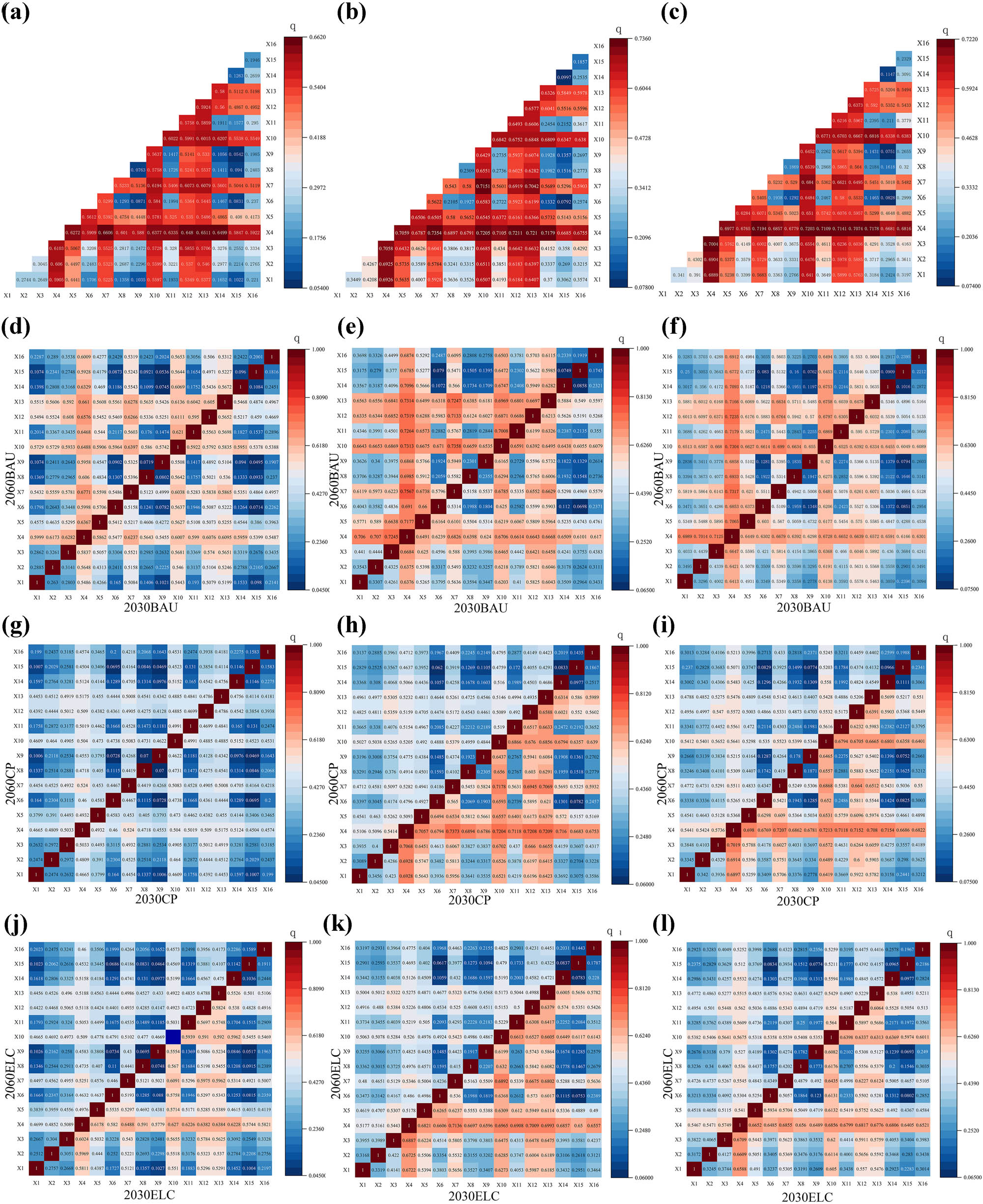
Interactivedetection of driving forces of each gradient band under sentimentality in 2030 and 2060; (d–l) is 2030 in the lower right corner and 2060 in the upper left corner. (a) 2020 Transition zones, (b) 2020, High ecological gradient zones, (c) 2020 High economic gradient zones, (d) (BAU) Transition zones, (e) (BAU) High ecological gradient zones, (f) (BAU) High economic gradient zones, (g) (CP) Transition zones, (h) (CP) High ecological gradient zones, (i) (CP) High economic gradient zones, (j) (ELC) Transition zones, (k) (ECL) High ecological gradient zones, and (l) (ECL) High economic gradient zones.
From 2030 to 2060, under both CP and ELC scenarios, the interactive effects of factors within each gradient zone on CS exhibited greater influence in 2030 compared to 2060. In 2030, under the CP scenario, the interactions of X4 with X5, X7, X10, X12, and X13 in the high economic and ecological gradient zones exerted a substantial influence on CS (0.70–0.75), while the transitional zone showed a moderate influence (0.50–0.55). Under the ELC scenario, the interactions of X4 with X7, X10, X12, and X13 demonstrated more pronounced effects on CS: high economic gradient zone (0.66–0.72) > high ecological gradient zone (0.66–0.69) > transitional zone (0.61–0.65). The interactive effects of factors X4, X7, and X10 on CS were higher in the high economic and ecological gradient zones (0.50–0.58) than in the transitional zone (0.47–0.52). Under the BAU scenario, the interactive effects of factors within each gradient zone on CS were greater in 2060 than in 2030. Additionally, the interactions of factors X4, X10, X12, and X13 in the high economic and ecological gradient zones (0.63–0.75) had a stronger influence than those in the transitional zone (0.60–0.67). This is because, under the BAU scenario, ecological and LUCC policy interventions were relatively limited, and the sustained advancement of urban economies exerted more pronounced cascading effects on ecological factors, thereby amplifying the impact on CS.
4.5 Heterogeneity of gradient space CS
This study calculated the root mean square deviations of economy, ecology, and CS for prefecture-level cities along three latitudinal-longitudinal belts in the YRD region in 2020. Wavelet variance analysis using the Morlet complex wavelet function revealed characteristic scales (Figure 20). The selection of analysis belts considered multidimensional factors, including north-south disparities, key economic-ecological interaction zones, and gradient transition belts, enabling more intuitive analysis of CS spatial heterogeneity from perspectives of geographical spatial variation, socioeconomics, and ecological value. Notably, in the Shanghai-Liuan (SL) belt, CS exhibited two distinct peaks with dominant periods in Suzhou and Changzhou, showing wavelet variances of 0.65–0.70. Economically, three prominent peaks appeared with dominant periods in Suzhou, Nanjing, and Hefei, displaying wavelet variances of 0.45–0.65. Ecologically, two peaks were observed with dominant periods in Suzhou and Nanjing, having wavelet variances of 0.25–0.35. Along the SL belt, CS exhibited varying fluctuation amplitudes in response to spatial heterogeneity between economy and ecology, demonstrating significant spatial heterogeneity. In the Zhoushan-Chizhou (ZC) belt, CS fluctuations were relatively minor without distinct peaks, with maximum values distributed in Ningbo and Huangshan (wavelet variance: 0.45). Economically, two significant peaks emerged, with dominant periods primarily in Ningbo and Hangzhou, showing wavelet variances of approximately 0.50–0.60, both representing high economic gradient zones along the ZC belt. Ecologically, a single prominent peak appeared with a dominant period in Hangzhou (wavelet variance: 0.65). The Xuzhou-Lishui (XL) belt spans the entire YRD region in a north-south direction. Along this belt, CS, economic, and ecological variances exhibited larger fluctuation amplitudes. CS displayed four distinct peaks with dominant periods in Suqian, Nanjing, Huangshan, and Quzhou. Economically, two prominent peaks emerged with dominant periods in Nanjing and Hangzhou, showing wavelet variances of 0.45 and 0.55, respectively, both representing critical high economic gradient zones. Ecologically, four significant peaks were observed with dominant periods in Huaian, Nanjing, Xuancheng, and Hangzhou, displaying notable variance differences (Huaian and Hangzhou wavelet variances: 0.35 and 0.67), indicating the most pronounced heterogeneity compared to surrounding regions.
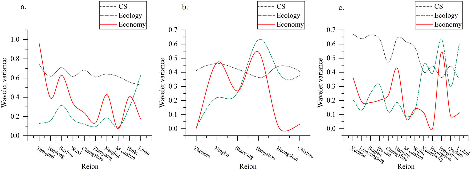
Feature detection for economic, ecological, and CS spatial heterogeneity. (a) SL, (b) ZC, and (c) XL.
5 Discussion
5.1 Effect of regional gradient differences on LUCC and CS
The YRD region covers a vast area and serves as the economic hub of China, characterized by a dense concentration of cities. Significant disparities exist in ecological environments and economic development, exhibiting gradient differentiation, with notable variations in LUCC within each gradient zone. The primary driver of CS changes is the alteration in LUCC types, as terrestrial surface conditions depend on LUCC, which subsequently induces ecological and environmental changes [61]. These changes ultimately affect the carbon cycle in ecosystem processes, leading to variations in CS. Over the past few decades, China has undergone rapid economic development, resulting in extensive vegetation destruction and ecosystem degradation [62]. As an economically advanced region, the YRD has experienced rapid urbanization, where urban expansion directly contributes to LUCC changes, accompanied by increased carbon emissions and carbon footprints [63]. During urban development in this region, the direction of urban sprawl also differentially impacts ecological corridors [64], habitat quality, and ecosystem services, leading to a reduction in ecological CS land and a significant decline in CS. Research indicates that from 2000 to 2020, the total CS in the YRD exhibited a declining trend, decreasing by 66.32 × 10⁶ t. The CS within the economic HGZ, ecological HGZ, and transition zone in the YRD region all show a downward trend to varying degrees, which is consistent with previous related studies on the changes in CS in the YRD region [65,66]. Projections suggest that this downward trend will persist from 2030 to 2060, albeit with a gradually diminishing rate of decline.
5.2 Driving force of CS spatial heterogeneity under gradient bands
Using the CatBoost-SHAP and OPGD models, this study analyzed the driving force characteristics of spatial heterogeneity in CS across the entire YRD region and its gradient zones. Previous studies have concluded that GDP and population are the primary factors contributing to the spatiotemporal differences in regional CS [67,68], which differs from the findings of this research. Single-factor analysis revealed that DEM and slope are the most significant drivers of CS variation in the YRD region, both at the regional level and within each gradient zone. Natural factors play a decisive role in the spatial heterogeneity of CS across the entire region and its gradient zones, particularly DEM, slope, NPP, vegetation type, and soil type. DEM and slope are the key determinants of regional CS changes. Significant differences in LUCC types exist at different elevations, directly influencing the CS of terrestrial ecosystems, which is consistent with previous research results [69]. In topographically complex areas with higher elevation and slope, human disturbance is relatively limited, vegetation coverage is favorable, and LUCC patterns remain relatively stable, creating an environment conducive to enhanced CS [70]. Due to the substantial differences in topography between the high economic gradient zone and the high ecological gradient zone – where the former is concentrated in low-altitude plains of Anhui and northern Jiangsu, while the latter is predominantly mountainous in western Anhui and Zhejiang – the influence of key driving factors such as DEM, slope, NPP, vegetation type, and soil type on CS exhibits minor fluctuations across the entire region and gradient zones, yet ecological factors remain dominant. Nighttime light, as an important socioeconomic factor, significantly impacts CS in the entire YRD region and the high economic gradient zone. GDP levels show a negative correlation with CS, as socioeconomic activities often entail excessive resource exploitation and environmental degradation, further leading to a decline in CS [71].
The analysis of driving factor interactions revealed that the combinations of DEM, slope, NPP, vegetation type, soil type, and soil-water conservation zones exerted highly significant impacts on CS across the entire region and within individual gradient zones. Since the distribution of vegetation types and soil types both depend on the changes in DEM and slope, and NPP depends on the distribution changes in vegetation and soil, DEM and slope are regarded as the ultimate dependent factors, which is consistent with the previous research results [72,73]. The interaction and combination with other factors have the most significant influence in each gradient zone. From 2000 to 2020, particularly from 2000 to 2010, the YRD region underwent rapid development. The high economic and ecological gradient zones occupied substantial areas of ecological land, such as forests and grasslands, leading to a weakened interactive effect between slope and DEM as primary factors and other driving factors, resulting in severe CS loss. In the 2030 and 2060 scenarios, with the further strengthening of spatial planning to enforce the protection of ecological land and CL, the interactions among DEM, slope, NPP, vegetation type, and soil type under the CP and ELC development scenarios will continue to mitigate the decline in CS in high economic gradient zones while promoting CS increases in high ecological gradient zones. In contrast, the high ecological gradient zone, located in the southwestern part of the YRD, is predominantly mountainous with lower population density, slower urban expansion, and better ecological conservation, generally maintaining more stable CS [74]. Therefore, from 2030 to 2060, further efforts should be made to enhance ecological and environmental protection.
Natural factors are the primary drivers influencing the heterogeneity of CS in the YRD region and its gradient zones, but the impact of anthropogenic factors should not be overlooked. The interactions among these factors exert complex and variable effects on the spatial heterogeneity of CS. This further underscores the necessity of prioritizing LUCC and ecological conservation policies in the formulation of National Territorial Spatial Planning, with full consideration given to the synergistic effects of different driving forces on CS enhancement.
5.3 Enlightenment of ecological protection and spatial planning in the YRD
This study reveals significant economic and ecological gradient variations in the YRD driven by socioeconomic and environmental heterogeneity. Notably, high economic gradient zones and high ecological gradient zones exhibit distinct LUCC patterns and CS distributions, with spatially imbalanced CS hindering regional carbon neutrality and ecological governance goals. Urbanization and land development are identified as primary drivers of CS decline. To enhance sustainable CS management, optimize LUCC planning, and strengthen ecosystem services, the following policy recommendations are proposed:
5.3.1 Gradient zoning control
Integrate gradient theory with multi-scale governance using territorial spatial information platforms, big data monitoring systems, and GIS to overcome administrative barriers in ecological and carbon management. Implement standardized dynamic zoning and scientific boundary delineation across the YRD to coordinate CS, ecological, and economic factors [75]. Develop differentiated policies for regional, intra-gradient, and provincial governance based on scenario-specific LUCC structures and gradient characteristics.
5.3.2 Strengthen the construction and management of key ecological service zones
The mountainous areas in the western and southern YRD, characterized by high ecological gradients and dense CS distribution, remain relatively undeveloped due to complex terrain. To safeguard these critical carbon sinks, we recommend enhancing ecological conservation in the southwestern mountainous regions by expanding key ecological protection zones and soil-water conservation areas while minimizing anthropogenic disturbances. Existing protected areas should undergo refined management to ensure long-term ecosystem stability and CS maintenance.
5.3.3 Strengthening the ecological and economic transformation and development of gradient zones
High economic gradient and transition zones: Strengthen CL protection by enforcing strict red lines in territorial spatial planning to curb urban encroachment. Improve agricultural eco-compensation mechanisms to encourage eco-friendly practices (e.g., organic farming, ecological agriculture), optimizing LUCC efficiency and mitigating CS loss from land conversion. Additionally, emphasize ecological civilization development by adhering to the “Two Mountains” theory (lucid waters and lush mountains are invaluable assets), promoting green industries to reduce pollution and emissions while ensuring CS stability [9]. High ecological gradient zones: Foster low-carbon, green economic transitions through sustainable models like eco-agriculture and ecotourism. These approaches can generate funding for ecological restoration while maintaining CS integrity.
5.3.4 Comprehensively promote sustainable urbanization in the YRD region
The eastern urban agglomerations, experiencing rapid urbanization and land development, exhibit relatively low CS levels. To balance low-carbon economic growth with CS preservation, we propose implementing a green urbanization strategy. Territorial spatial planning should prioritize green space optimization, expanding urban greenbelts, and ecological corridors to enhance carbon sequestration. Concurrently, ecological restoration projects along rivers, lakes, and coastal areas – particularly wetlands and forests – should be intensified to leverage natural ecosystems for CS improvement [76].
5.4 Research limitations and future themes
This study employed a coupled modeling approach (PLUS-InVEST, CatBoost-SHAP, and OPGD-WA) to analyze spatiotemporal patterns and driving forces of CS across gradient zones in the YRD under different development scenarios, providing new perspectives for regional CS assessment. PLUS model’s land transition rules, based on historical data, may not reflect long-term future changes – future studies should refine parameters for improved LUCC simulation accuracy [74]. InVEST’s CS module uses static LUCC-based estimates without considering carbon cycle dynamics or inter-pool transfers [77]. Static carbon density values in InVEST ignore detailed land-use types’ sequestration capacity and vegetation growth/seasonal variations [78]. Finally, no further research was conducted on the risk prediction and assessment of CS losses. In future research, the carbon sequestration capacity of detailed land use types should be incorporated. Second, attention should be paid to the changes in CS caused by the growth variations in plants and seasonal changes. Meanwhile, the impact of geological disasters and meteorological disasters on CS can be introduced to further enhance the comprehensive risk assessment of CS losses and establish a complete risk assessment system for CS vulnerability [79]. Our goal is to provide more realistic, accurate, and comprehensive assessment results.
6 Conclusion
This study integrates the PLUS-InVEST and CatBoost-SHAP-Geodetector-WV models. From the perspective of regional economic and ecological gradient variations, it elucidates the driving mechanisms and spatial heterogeneity affecting CS changes in economic-ecological gradient zones under different scenarios. The results indicate that
From 2000 to 2020, WL and CL decreased significantly, while BL area increased substantially. The overall CS exhibited a fluctuating downward trend, with the most pronounced decline occurring in high economic gradient zones, reaching its minimum value by 2020.
From 2020 to 2060, under the BAU scenario, CS exhibits a declining trend, with the rate of decline slowing across the entire region. The CS reduction in high economic gradient zones is more pronounced than in high ecological gradient zones. Under the CP and ELC scenarios, CS demonstrates a “decrease followed by an increase” trend, reaching its lowest point in 2030. From 2030 to 2060, CS gradually increases, with the growth rate under the ELC scenario surpassing that of the CP scenario. The most significant CS increase occurs in high ecological gradient zones.
The fluctuations of CS within the gradient zone show significant spatial heterogeneity. The fluctuation changes in CS correspond to the economic and ecological fluctuation changes in the region. They are not only constrained by the natural background but also closely related to the integrated development policy of the YRD region. The economic HGZ fluctuates the most, while the ecological HGZ is relatively stable. CS generally shows a state of increasing from the coast to the inland and a decrease from south to north. In terms of total volume, the CS in the ecological HGZ has always been 50% higher than that in the economic HGZ. Essentially, it is the result of the transformation of China’s regional development strategy from unbalanced development to coordinated development. The policy of the integration of the YRD has reshaped the regional development dynamic mechanism by systematically optimizing resource allocation, directly influencing the evolution direction of the economic and ecological gradients. The economic ecology of the special areas is at a relatively high level, with a large CS and a low fluctuation coefficient. In the future, it will be the first to become a carbon neutrality area in the YRD region.
DEM, slope, NPP, vegetation type, soil type, and nighttime light exhibited the most significant impacts on CS. Under the CP and ELC scenarios, the interaction of DEM, slope, and NPP exerted the strongest driving force on CS growth. Slope and DEM demonstrated the highest explanatory power for CS within gradient zones.
This research framework provides a new management direction for regional ecological CS and National Territorial Spatial Ecological Governance. Breaking through the traditional research on spatial heterogeneity, it integrates socio-economic indicators based on the “landscape gradient theory,” and constructs a comprehensive evaluation framework that takes into account socio-economic, CS, and ecological protection. In the future, the entire “identification – diagnosis – optimization” process of gradient LUCC and CS should be incorporated into the decision-making for regional ecological environment governance and CS management, based on the "gradient transition" characteristics of regional CS loss.
-
Funding information: This work was supported by the Open Fund of Zhejiang Provincial Key Laboratory of Resource and Environment Information System (Grant No. ZJGIS-KFJJ-20230301) and the Open Fund of Wenzhou Future City Research Institute (Grant No. WL2023012).
-
Author contributions: Xuankai Huang: Writing the original draft, visualization, validation, methodology, and formal analysis. Xiaomin Jiang: Writing – review and editing, supervision, project administration, funding acquisition, and conceptualization. Binjie Zhou: Data curation, resources and methodology. Ling Yang: Investigation, software, writing – review and editing.
-
Conflict of interest: Authors state no conflict of interest.
References
[1] Zhang YJ, Liu Z, Zhang H, Tan TD. The impact of economic growth, industrial structure, and urbanization on carbon emission intensity in China. Nat Hazards. 2014;73:579–95. 10.1007/s11069-014-1091-x.Search in Google Scholar
[2] Fox-Kemper B, Hewitt HT, Xiao C, Aðalgeirsdóttir G, Drijfhout SS, Edwards TL, et al. Climate change 2021: The physical science basis. Contribution of working group I to the sixth assessment report of the intergovernmental panel on climate change. Berlin, Germany: Cambridge University Press; 2021.Search in Google Scholar
[3] Chen G, Li X, Liu X, Chen Y, Liang X, Leng J, et al. Global projections of future urban land expansion under shared socioeconomic pathways. Nat Commun. 2020;11:537. 10.1038/s41467-020-14386-x.Search in Google Scholar PubMed PubMed Central
[4] Yang P, Tang KW, Yang H, Tong C, Yang N, Lai DYF, et al. Insights into the farming-season carbon budget of coastal earthen aquaculture ponds in southeastern China. Agric Ecosyst Environ. 2022;335:107995. 10.1016/j.agee.2022.107995.Search in Google Scholar
[5] Tian Z, Mu X. Towards China’s dual-carbon target: Energy efficiency analysis of cities in the Yellow River Basin based on a “geography and high-quality development” heterogeneity framework. Energy. 2024;306:132396. 10.1016/j.energy.2024.132396.Search in Google Scholar
[6] Wang N, Chen X, Zhang Y, Pang J, Long Z, Chen Y, et al. Integrated effects of land use and land cover change on carbon metabolism: Based on ecological network analysis. Environ Impact Assess Rev. 2024;104:107320. 10.1016/j.eiar.2023.107320.Search in Google Scholar
[7] Kafy AA, Abdullah-Al-Faisal AF, Rahman MS, Islam M, Al Rakib A, Islam MA, et al. Prediction of seasonal urban thermal field variance index using machine learning algorithms in Cumilla, Bangladesh. Sustain Cities Soc. 2021;64:102542. 10.1016/j.scs.2020.102542.Search in Google Scholar
[8] García-Ontiyuelo M, Acuña-Alonso C, Valero E, Álvarez X. Geospatial mapping of carbon estimates for forested areas using the InVEST model and Sentinel-2: A case study in Galicia (NW Spain). Sci Total Environ. 2024;922:171297. 10.1016/j.scitotenv.2024.171297.Search in Google Scholar PubMed
[9] Wu Q, Wang L, Wang T, Ruan Z, Du P. Spatial–temporal evolution analysis of multi-scenario land use and carbon storage based on PLUS-InVEST model: A case study in Dalian, China. Ecol Indic. 2024;166:112448. 10.1016/j.ecolind.2024.112448.Search in Google Scholar
[10] Zhong Q, Ma J, Zhao B, Wang X, Zong J, Xiao X. Assessing spatial-temporal dynamics of urban expansion, vegetation greenness and photosynthesis in megacity Shanghai, China during 2000–2016. Remote Sens Environ. 2019;233:111374. 10.1016/j.rse.2019.111374.Search in Google Scholar
[11] Peng X, Jiang S, Liu S, Valbuena R, Smith A, Zhan Y, et al. Long-term satellite observations show continuous increase of vegetation growth enhancement in urban environment. Sci Total Environ. 2023;898:165515. 10.1016/j.scitotenv.2023.165515.Search in Google Scholar PubMed
[12] Xu Y, Zhao X, Huang P, Pu J, Ran Y, Zhou S, et al. A new framework for multi-level territorial spatial zoning management: Integrating ecosystem services supply-demand balance and land use structure. J Clean Prod. 2024;441:141053. 10.1016/j.jclepro.2024.141053.Search in Google Scholar
[13] Sha ZY, Bai YF, Li RR, Lan H, Zhang XL, Li J, et al. The global carbon sink potential of terrestrial vegetation can be increased substantially by optimal land management. Commun Earth Environ. 2022;3:1–10. 10.1038/s43247-021-00333-1.Search in Google Scholar
[14] Piao S, Fang J, Ciais P, Peylin P, Huang Y, Sitch S, et al. The carbon balance of terrestrial ecosystems in China. Nature. 2009;458:1009–13. 10.1038/nature07944.Search in Google Scholar PubMed
[15] Tang X, Zhao X, Bai Y, Tang Z, Wang W, Zhao Y, et al. Carbon pools in China’s terrestrial ecosystems: New estimates based on an intensive field survey. Proc Natl Acad Sci U S A. 2018;115:4021–6. 10.1073/pnas.1700291115.Search in Google Scholar PubMed PubMed Central
[16] Wang A, Kafy AA, Rahaman ZA, Rahman MT, Faisal AA, Afroz F. Investigating drivers impacting vegetation carbon sequestration capacity on the terrestrial environment in 127 Chinese cities. Environ Sustain Indic. 2022;16:100213. 10.1016/j.indic.2022.100213.Search in Google Scholar
[17] Viña A, McConnell WJ, Yang H, Xu Z, Liu J. Effects of conservation policy on China’s forest recovery. Sci Adv. 2016;2:1500965. 10.1126/sciadv.1500965.Search in Google Scholar PubMed PubMed Central
[18] Kong L, Zheng H, Rao E, Xiao Y, Ouyang Z, Li C. Evaluating indirect and direct effects of eco-restoration policy on soil conservation service in the Yangtze River Basin. Sci Total Environ. 2018;631–632:887–94. 10.1016/j.scitotenv.2018.03.117.Search in Google Scholar PubMed
[19] Yu P, Zhang S, Yung EHK, Chan EHW, Luan B, Chen Y. On the urban compactness to ecosystem services in a rapidly urbanising metropolitan area: Highlighting scale effects and spatial non–stationary. Environ Impact Assess Rev. 2023;98:106975. 10.1016/j.eiar.2022.106975.Search in Google Scholar
[20] Nie Q, Wu G, Li L, Man W, Ma J, Bao Z, et al. Exploring scaling differences and spatial heterogeneity in drivers of carbon storage Changes: A comprehensive geographic analysis framework. Ecol Indic. 2024;165:112193. 10.1016/j.ecolind.2024.112193.Search in Google Scholar
[21] Madigan AP, Zimmermann J, Krol DJ, Williams M, Jones MB. Full Inversion Tillage (FIT) during pasture renewal as a potential management strategy for enhanced carbon sequestration and storage in Irish grassland soils. Sci Total Environ. 2022;805:150342. 10.1016/j.scitotenv.2021.150342.Search in Google Scholar PubMed
[22] Fryer J, Williams ID. Regional carbon stock assessment and the potential effects of land cover change. Sci Total Environ. 2021;775:145815. 10.1016/j.scitotenv.2021.145815.Search in Google Scholar PubMed
[23] Li L, Song Y, Wei XH, Dong J. Exploring the impacts of urban growth on carbon storage under integrated spatial regulation: A case study of Wuhan, China. Ecol Indic. 2020;111:106064. 10.1016/j.ecolind.2020.106064.Search in Google Scholar
[24] Wu W, Xu L, Zheng H, Zhang X. How much carbon storage will the ecological space leave in a rapid urbanization area? Scenario analysis from Beijing-Tianjin-Hebei Urban Agglomeration. Resour Conserv Recycl. 2023;189:106774. 10.1016/j.resconrec.2022.106774.Search in Google Scholar
[25] Jia L, Yu K, Li Z, Li P, Xu G, Cong P, et al. Spatiotemporal pattern of NPP and its response to climatic factors in the Yangtze River Economic Belt. Ecol Indic. 2024;162:112017. 10.1016/j.ecolind.2024.112017.Search in Google Scholar
[26] Yang XD, Li HL, Zhang JY, Niu SY, Miao MM. Urban economic resilience within the Yangtze River Delta urban agglomeration: Exploring spatially correlated network and spatial heterogeneity. Sustain Cities Soc. 2024;103:105270. 10.1016/j.scs.2024.105270.Search in Google Scholar
[27] Lu Y, Wang J, Jiang X. Spatial and temporal changes of ecosystem service value and it’s influencing mechanism in the Yangtze River Delta urban agglomeration. Sci Rep. 2024;14:19476. 10.1038/s41598-024-70248-2.Search in Google Scholar PubMed PubMed Central
[28] Vaughn RM, Hostetler M, Escobedo FJ, Jones P. The influence of subdivision design and conservation of open space on carbon storage and sequestration. Landsc Urban Plan. 2014;131:64–73. 10.1016/j.landurbplan.2014.08.001.Search in Google Scholar
[29] Chen W, Wang G, Gu T, Fang C, Pan S, Zeng J, et al. Simulating the impact of urban expansion on ecosystem services in Chinese urban agglomerations: A multi-scenario perspective. Environ Impact Assess Rev. 2023;103:107275. 10.1016/j.eiar.2023.107275.Search in Google Scholar
[30] Liu G, Zhang F. How to do trade-offs between urban expansion and ecological construction influence CO2 emissions? New evidence from China. Ecol Indic. 2022;141:109070. 10.1016/j.ecolind.2022.109070.Search in Google Scholar
[31] Chung SY, Ives MC, Allen MR, Doorga JRS, Xu Y. Accelerating carbon neutrality in China: Sensitive intervention points for the energy and transport sectors in Beijing and Hong Kong. J Clean Prod. 2024;450:141681. 10.1016/j.jclepro.2024.141681.Search in Google Scholar
[32] Guo L, Tang M, Wu Y, Bao S, Wu Q. Government-led regional integration and economic growth: Evidence from a quasi-natural experiment of urban agglomeration development planning policies in China. Cities. 2025;156:105482. 10.1016/j.cities.2024.105482.Search in Google Scholar
[33] Zhang C, Ji J, Li R, Zhang D, Streimikiene D. Determinants and spatial spillover of inter-provincial carbon leakage in China: The perspective of economic cycles. Technol Forecast Soc Change. 2023;194:122678. 10.1016/j.techfore.2023.122678.Search in Google Scholar
[34] Qureshi S, Haase D, Coles R. The theorized urban gradient (TUG) method—a conceptual framework for socio-ecological sampling in complex urban agglomerations. Ecol Indic. 2014;36:100–10. 10.1016/j.ecolind.2013.07.010.Search in Google Scholar
[35] Zhang H, Li X, Luo Y, Chen L, Wang M. Spatial heterogeneity and driving mechanisms of carbon storage in the urban agglomeration within complex terrain: Multi-scale analyses under localized SSP-RCP narratives. Sustain Cities Soc. 2024;109:105520. 10.1016/j.scs.2024.105520.Search in Google Scholar
[36] Forman G. Landscape ecology. New York: John Wiley and Sons Ltd.; 1986.Search in Google Scholar
[37] Wei M, Cai Z, Song Y, Xu J, Lu M. Spatiotemporal evolutionary characteristics and driving forces of carbon emissions in three Chinese urban agglomerations. Sustain Cities Soc. 2024;104:105320. 10.1016/j.scs.2024.105320.Search in Google Scholar
[38] Wang H, Wu L, Yue Y, Jin Y, Zhang B. Impacts of climate and land use change on terrestrial carbon storage: A multi-scenario case study in the Yellow River Basin (1992–2050). Sci Total Environ. 2024;930:172557. 10.1016/j.scitotenv.2024.172557.Search in Google Scholar PubMed
[39] Wang Y, Liang D, Wang J, Zhang Y, Chen F, Ma X. An analysis of regional carbon stock response under land use structure change and multi-scenario prediction, a case study of Hefei, China. Ecol Indic. 2023;151:110293. 10.1016/j.ecolind.2023.110293.Search in Google Scholar
[40] Zafar Z, Zubair M, Zha Y, Mehmood MS, Rehman A, Fahd S, et al. Predictive modeling of regional carbon storage dynamics in response to land use/land cover changes: An InVEST-based analysis. Ecol Inform. 2024;82:102701. 10.1016/j.ecoinf.2024.102701.Search in Google Scholar
[41] Wu D, Mo J, Zeng L, Zhou P, Xie M, Yuan H. Ecosystem services scenario simulation in Guangzhou based on the FLUS-InVEST model. Sci Rep. 2025;15:14054. 10.1038/s41598-025-98248-w.Search in Google Scholar PubMed PubMed Central
[42] Shao Z, Chen R, Zhao J, Xia CY, He YT, Tang FY. Spatio-temporal evolution and prediction of carbon storage in Beijing’s ecosystem based on FLUS and InVEST models. Acta Ecol Sin. 2022;42:9456–69. 10.5846/stxb202201100094.Search in Google Scholar
[43] Tong RX, Liang X, Guan QF, Song Y, Chen YL, Wang QY, et al. Estimation of soil carbon storage change from land use and management at a high spatial resolution in China during 2000–2020. Acta Geogr Sin. 2023;78:2209–22. 10.11821/dlxb202309006.Search in Google Scholar
[44] Zhang YX, Wang XJ, Pu Y, Zhang JB. Changes in forest resource carbon storage in China between 1949 and 2018. J Beijing For Univ. 2021;43:1–14. 10.12171/j.1000-1522.20200237.Search in Google Scholar
[45] Hou R, Xia C, Chen J, Zheng Q, Li H, Huang J, et al. Carbon storage and carbon sink of forest land and other biomass in the Yangtze River Economic Belt. Acta Ecol Sin. 2022;42:9483–98. 10.5846/stxb202201140134.Search in Google Scholar
[46] Cavallaro F, Zavadskas E, Raslanas S. Evaluation of combined heat and power (CHP) systems using fuzzy Shannon entropy and fuzzy TOPSIS. Sustainability. 2016;8:556. 10.3390/su8060556.Search in Google Scholar
[47] Pan XH, Wang YM. An enhanced technique for order preference by similarity to ideal solutions and its application to renewable energy resources selection problem. Int J Fuzzy Syst. 2020;23:1087–101. 10.1007/s40815-020-00914-w.Search in Google Scholar
[48] Chen C, He X, Liu Z, Sun W, Dong H, Chu Y. Analysis of regional economic development based on land use and land cover change information derived from Landsat imagery. Sci Rep. 2020;10:12721. 10.1038/s41598-020-69716-2.Search in Google Scholar PubMed PubMed Central
[49] Deng G, Jiang H, Zhu S, Wen Y, He C, Wang X, et al. Projecting the response of ecological risk to land use/land cover change in ecologically fragile regions. Sci Total Environ. 2024;914:169908. 10.1016/j.scitotenv.2024.169908.Search in Google Scholar PubMed
[50] Liu J, Zhou Y, Wang L, Zuo Q, Li Q, He N. Spatiotemporal analysis and multi-scenario prediction of ecosystem services based on land use/cover change in a Mountain-Watershed Region, China. Remote Sens. 2023;15:2759. 10.3390/rs15112759.Search in Google Scholar
[51] Xu X, Zhang Z, Long T, Sun S, Gao J. Mega-city region sustainability assessment and obstacles identification with GIS–entropy–TOPSIS model: A case in Yangtze River Delta urban agglomeration, China. J Clean Prod. 2021;294:126147. 10.1016/j.jclepro.2021.126147.Search in Google Scholar
[52] Zhang H, Gu C-L, Gu L-W, Zhang Y. The evaluation of tourism destination competitiveness by TOPSIS & information entropy–A case in the Yangtze River Delta of China. Tour Manag. 2011;32:443–51. 10.1016/j.tourman.2010.02.007.Search in Google Scholar
[53] Chen J, You J, Wei J, Dai Z, Zhang G. Interpreting XGBoost predictions for shear-wave velocity using SHAP: Insights into gas hydrate morphology and saturation. Fuel. 2024;364:131145. 10.1016/j.fuel.2024.131145.Search in Google Scholar
[54] Prokhorenkova L, Gusev G, Vorobev A, Dorogush AV, Gulin A. CatBoost: Unbiased boosting with categorical features. Mach Learn. 2017;31:1–23. 10.48550/ARXIV.1706.09516.Search in Google Scholar
[55] Lundberg SM, Nair B, Vavilala MS, Horibe M, Eisses MJ, Adams T, et al. Explainable machine-learning predictions for the prevention of hypoxaemia during surgery. Nat Biomed Eng. 2018;2:749–60. 10.1038/s41551-018-0304-0.Search in Google Scholar PubMed PubMed Central
[56] Lloyd SS. A value for n-person games. Princeton: Princeton University Press; 1953.Search in Google Scholar
[57] Wang JF, Li XH, Christakos G, Liao YL, Zhang T, Gu X, et al. Geographical detectors‐based health risk assessment and its application in the neural tube defects study of the Heshun Region, China. Int J Geogr Inf Sci. 2010;24:107–27. 10.1080/13658810802443457.Search in Google Scholar
[58] David M, Mah M. The use of wavelets for spatial pattern analysis in ecology. J Veg Sci. 1998;9:805–14. 10.2307/3237046.Search in Google Scholar
[59] Xie J, Liu T, Wei P, Jia Y, M, Luo C. Ecological application of wavelet analysis in the scaling of spatial distribution patterns of Ceratoides ewersmanniana. Acta Ecol Sin. 2007;27:2704–14. 10.1016/S1872-2032(07)60058-4.Search in Google Scholar
[60] Zhang N, Zhang H. Scale variance analysis coupled with Moran’s I scalogram to identify hierarchy and characteristic scale. Int J Geogr Inf Sci. 2011;25:1525–43. 10.1080/13658816.2010.532134.Search in Google Scholar
[61] Lu F, Hu H, Sun W, Zhu J, Liu G, Zhou W, et al. Effects of national ecological restoration projects on carbon sequestration in China from 2001 to 2010. Proc Natl Acad Sci U S A. 2018;115:4039–44. 10.1073/pnas.1700294115.Search in Google Scholar PubMed PubMed Central
[62] Ouyang Z, Zheng H, Xiao Y, Polasky S, Liu J, Xu W, et al. Improvements in ecosystem services from investments in natural capital. Science. 2016;352:1455–9. 10.1126/science.aaf2295.Search in Google Scholar PubMed
[63] Hutyra LR, Yoon B, Hepinstall-Cymerman J, Alberti M. Carbon consequences of land cover change and expansion of urban lands: A case study in the Seattle metropolitan region. Landsc urban Plan. 2011;103:83–93. 10.1016/j.landurbplan.2011.06.004.Search in Google Scholar
[64] Wang J, Shao Z, Fu P, Zhuang Q, Chang J, Jing P, et al. Unraveling the impact of urban expansion on vegetation carbon sequestration capacity: A case study of the Yangtze River Economic Belt. Sustain Cities Soc. 2025;120:106157. 10.1016/j.scs.2025.106157.Search in Google Scholar
[65] Wei Z, Li J, Wang Z, Zhou A, Li M. County carbon emissions in the Yangtze River Delta region: spatial layout, dynamic evolution and spatial spillover effects. Front Environ Sci. 2022;10:977198. 10.3389/fenvs.2022.977198.Search in Google Scholar
[66] Zhou ZC, Wang J. Evolution of landscape dynamics in the Yangtze River Delta from 2000 to 2020. J Water Clim Change. 2022;13:1241–56. 10.2166/wcc.2022.307.Search in Google Scholar
[67] Fu K, Chen L, Yu X, Jia G. How has carbon storage changed in the Yili-Tianshan region over the past three decades and into the future? What has driven it to change? Sci Total Environ. 2024;945:174005. 10.1016/j.scitotenv.2024.174005.Search in Google Scholar PubMed
[68] Wei H, Xiong L, Tang G, Strobl J, Xue K. Spatial–temporal variation of land use and land cover change in the glacial-affected area of the Tianshan Mountains. Catena. 2021;202:105256. 10.1016/j.catena.2021.105256.Search in Google Scholar
[69] Yang X, Bai X, Yao W, Li P, Hu J, Kang L. Spatioemporal dynamics and driving forces of soil organic carbon changes in an arid coal mining area of China investigated based on remote sensing techniques. Ecol Indic. 2024;158:111453. 10.1016/j.ecolind.2023.111453.Search in Google Scholar
[70] Jia X, Zhu J, Li Y, Wu W, Hu X. Analysis of the driving role and impact of road construction on carbon stock. Environ Sci Pollut Res Int. 2023;30:67131–49. 10.1007/s11356-023-27198-5.Search in Google Scholar PubMed
[71] Shen Z, Tiruta-Barna L, Karan SK, Hamelin L. Simultaneous carbon storage in arable land and anthropogenic products (CSAAP): Demonstrating an integrated concept towards well below 2°C. Resour Conserv Recycl. 2022;182:106293. 10.1016/j.resconrec.2022.106293.Search in Google Scholar
[72] Huang F, Xiong H, Jiang S-H, Yao C, Fan X, Catani F, et al. Modelling landslide susceptibility prediction: A review and construction of semi-supervised imbalanced theory. Earth-Sci Rev. 2024;250:104700. 10.1016/j.earscirev.2024.104700.Search in Google Scholar
[73] Mousavi SR, Sarmadian F, Angelini ME, Bogaert P, Omid M. Cause-effect relationships using structural equation modeling for soil properties in arid and semi-arid regions. Catena. 2023;232:107392. 10.1016/j.catena.2023.107392.Search in Google Scholar
[74] Zhu WB, Zhang JJ, Cui YP, Zhu LP. Ecosystem carbon storage under different scenarios of land use change in Qihe catchment, China. J Geogr Sci. 2020;30:1507–22. 10.1007/s11442-020-1796-6.Search in Google Scholar
[75] Wu Q, Cao Y, Su D, Cao Y. A multi-scale framework for understanding spatial scale effects on ecosystem service heterogeneity, interactions, drivers, and their socio-ecological impact pathways for adaptive management. J Clean Prod. 2025;516:145757. 10.1016/j.jclepro.2025.145757.Search in Google Scholar
[76] Wang X-L, Feng A-Q, Hou X-Y, Chao Q-C, Song B-Y, Liu Y-B, et al. Compound extreme inundation risk of coastal wetlands caused by climate change and anthropogenic activities in the Yellow River Delta, China. Adv Clim Change Res. 2024;15:134–47. 10.1016/j.accre.2024.01.010.Search in Google Scholar
[77] Fan L, Cai T, Wen Q, Han J, Wang S, Wang J, et al. Scenario simulation of land use change and carbon storage response in Henan Province, China: 1990–2050. Ecol Indic. 2023;154:110660. 10.1016/j.ecolind.2023.110660.Search in Google Scholar
[78] Jin T, Zhang P, Zhou N, Li S. Unveiling the spatiotemporal heterogeneity and driving mechanisms of carbon storage changes in response to land use/land cover changes under different future scenarios: Insights from the GMOP-SEM model. J Clean Prod. 2025;487:144622. 10.1016/j.jclepro.2024.144622.Search in Google Scholar
[79] Huang F, Liu K, Li Z, Zhou X, Zeng Z, Li W, et al. Single landslide risk assessment considering rainfall‐induced landslide hazard and the vulnerability of disaster‐bearing body. Geol J. 2024;59:2549–65. 10.1002/gj.4976.Search in Google Scholar
© 2025 the author(s), published by De Gruyter
This work is licensed under the Creative Commons Attribution 4.0 International License.
Articles in the same Issue
- Research Articles
- Seismic response and damage model analysis of rocky slopes with weak interlayers
- Multi-scenario simulation and eco-environmental effect analysis of “Production–Living–Ecological space” based on PLUS model: A case study of Anyang City
- Remote sensing estimation of chlorophyll content in rape leaves in Weibei dryland region of China
- GIS-based frequency ratio and Shannon entropy modeling for landslide susceptibility mapping: A case study in Kundah Taluk, Nilgiris District, India
- Natural gas origin and accumulation of the Changxing–Feixianguan Formation in the Puguang area, China
- Spatial variations of shear-wave velocity anomaly derived from Love wave ambient noise seismic tomography along Lembang Fault (West Java, Indonesia)
- Evaluation of cumulative rainfall and rainfall event–duration threshold based on triggering and non-triggering rainfalls: Northern Thailand case
- Pixel and region-oriented classification of Sentinel-2 imagery to assess LULC dynamics and their climate impact in Nowshera, Pakistan
- The use of radar-optical remote sensing data and geographic information system–analytical hierarchy process–multicriteria decision analysis techniques for revealing groundwater recharge prospective zones in arid-semi arid lands
- Effect of pore throats on the reservoir quality of tight sandstone: A case study of the Yanchang Formation in the Zhidan area, Ordos Basin
- Hydroelectric simulation of the phreatic water response of mining cracked soil based on microbial solidification
- Spatial-temporal evolution of habitat quality in tropical monsoon climate region based on “pattern–process–quality” – a case study of Cambodia
- Early Permian to Middle Triassic Formation petroleum potentials of Sydney Basin, Australia: A geochemical analysis
- Micro-mechanism analysis of Zhongchuan loess liquefaction disaster induced by Jishishan M6.2 earthquake in 2023
- Prediction method of S-wave velocities in tight sandstone reservoirs – a case study of CO2 geological storage area in Ordos Basin
- Ecological restoration in valley area of semiarid region damaged by shallow buried coal seam mining
- Hydrocarbon-generating characteristics of Xujiahe coal-bearing source rocks in the continuous sedimentary environment of the Southwest Sichuan
- Hazard analysis of future surface displacements on active faults based on the recurrence interval of strong earthquakes
- Structural characterization of the Zalm district, West Saudi Arabia, using aeromagnetic data: An approach for gold mineral exploration
- Research on the variation in the Shields curve of silt initiation
- Reuse of agricultural drainage water and wastewater for crop irrigation in southeastern Algeria
- Assessing the effectiveness of utilizing low-cost inertial measurement unit sensors for producing as-built plans
- Analysis of the formation process of a natural fertilizer in the loess area
- Machine learning methods for landslide mapping studies: A comparative study of SVM and RF algorithms in the Oued Aoulai watershed (Morocco)
- Chemical dissolution and the source of salt efflorescence in weathering of sandstone cultural relics
- Molecular simulation of methane adsorption capacity in transitional shale – a case study of Longtan Formation shale in Southern Sichuan Basin, SW China
- Evolution characteristics of extreme maximum temperature events in Central China and adaptation strategies under different future warming scenarios
- Estimating Bowen ratio in local environment based on satellite imagery
- 3D fusion modeling of multi-scale geological structures based on subdivision-NURBS surfaces and stratigraphic sequence formalization
- Comparative analysis of machine learning algorithms in Google Earth Engine for urban land use dynamics in rapidly urbanizing South Asian cities
- Study on the mechanism of plant root influence on soil properties in expansive soil areas
- Simulation of seismic hazard parameters and earthquakes source mechanisms along the Red Sea rift, western Saudi Arabia
- Tectonics vs sedimentation in foredeep basins: A tale from the Oligo-Miocene Monte Falterona Formation (Northern Apennines, Italy)
- Investigation of landslide areas in Tokat-Almus road between Bakımlı-Almus by the PS-InSAR method (Türkiye)
- Predicting coastal variations in non-storm conditions with machine learning
- Cross-dimensional adaptivity research on a 3D earth observation data cube model
- Geochronology and geochemistry of late Paleozoic volcanic rocks in eastern Inner Mongolia and their geological significance
- Spatial and temporal evolution of land use and habitat quality in arid regions – a case of Northwest China
- Ground-penetrating radar imaging of subsurface karst features controlling water leakage across Wadi Namar dam, south Riyadh, Saudi Arabia
- Rayleigh wave dispersion inversion via modified sine cosine algorithm: Application to Hangzhou, China passive surface wave data
- Fractal insights into permeability control by pore structure in tight sandstone reservoirs, Heshui area, Ordos Basin
- Debris flow hazard characteristic and mitigation in Yusitong Gully, Hengduan Mountainous Region
- Research on community characteristics of vegetation restoration in hilly power engineering based on multi temporal remote sensing technology
- Identification of radial drainage networks based on topographic and geometric features
- Trace elements and melt inclusion in zircon within the Qunji porphyry Cu deposit: Application to the metallogenic potential of the reduced magma-hydrothermal system
- Pore, fracture characteristics and diagenetic evolution of medium-maturity marine shales from the Silurian Longmaxi Formation, NE Sichuan Basin, China
- Study of the earthquakes source parameters, site response, and path attenuation using P and S-waves spectral inversion, Aswan region, south Egypt
- Source of contamination and assessment of potential health risks of potentially toxic metal(loid)s in agricultural soil from Al Lith, Saudi Arabia
- Regional spatiotemporal evolution and influencing factors of rural construction areas in the Nanxi River Basin via GIS
- An efficient network for object detection in scale-imbalanced remote sensing images
- Effect of microscopic pore–throat structure heterogeneity on waterflooding seepage characteristics of tight sandstone reservoirs
- Environmental health risk assessment of Zn, Cd, Pb, Fe, and Co in coastal sediments of the southeastern Gulf of Aqaba
- A modified Hoek–Brown model considering softening effects and its applications
- Evaluation of engineering properties of soil for sustainable urban development
- The spatio-temporal characteristics and influencing factors of sustainable development in China’s provincial areas
- Application of a mixed additive and multiplicative random error model to generate DTM products from LiDAR data
- Gold vein mineralogy and oxygen isotopes of Wadi Abu Khusheiba, Jordan
- Prediction of surface deformation time series in closed mines based on LSTM and optimization algorithms
- 2D–3D Geological features collaborative identification of surrounding rock structural planes in hydraulic adit based on OC-AINet
- Spatiotemporal patterns and drivers of Chl-a in Chinese lakes between 1986 and 2023
- Land use classification through fusion of remote sensing images and multi-source data
- Nexus between renewable energy, technological innovation, and carbon dioxide emissions in Saudi Arabia
- Analysis of the spillover effects of green organic transformation on sustainable development in ethnic regions’ agriculture and animal husbandry
- Factors impacting spatial distribution of black and odorous water bodies in Hebei
- Large-scale shaking table tests on the liquefaction and deformation responses of an ultra-deep overburden
- Impacts of climate change and sea-level rise on the coastal geological environment of Quang Nam province, Vietnam
- Reservoir characterization and exploration potential of shale reservoir near denudation area: A case study of Ordovician–Silurian marine shale, China
- Seismic prediction of Permian volcanic rock reservoirs in Southwest Sichuan Basin
- Application of CBERS-04 IRS data to land surface temperature inversion: A case study based on Minqin arid area
- Geological characteristics and prospecting direction of Sanjiaoding gold mine in Saishiteng area
- Research on the deformation prediction model of surrounding rock based on SSA-VMD-GRU
- Geochronology, geochemical characteristics, and tectonic significance of the granites, Menghewula, Southern Great Xing’an range
- Hazard classification of active faults in Yunnan base on probabilistic seismic hazard assessment
- Characteristics analysis of hydrate reservoirs with different geological structures developed by vertical well depressurization
- Estimating the travel distance of channelized rock avalanches using genetic programming method
- Landscape preferences of hikers in Three Parallel Rivers Region and its adjacent regions by content analysis of user-generated photography
- New age constraints of the LGM onset in the Bohemian Forest – Central Europe
- Characteristics of geological evolution based on the multifractal singularity theory: A case study of Heyu granite and Mesozoic tectonics
- Soil water content and longitudinal microbiota distribution in disturbed areas of tower foundations of power transmission and transformation projects
- Oil accumulation process of the Kongdian reservoir in the deep subsag zone of the Cangdong Sag, Bohai Bay Basin, China
- Investigation of velocity profile in rock–ice avalanche by particle image velocimetry measurement
- Optimizing 3D seismic survey geometries using ray tracing and illumination modeling: A case study from Penobscot field
- Sedimentology of the Phra That and Pha Daeng Formations: A preliminary evaluation of geological CO2 storage potential in the Lampang Basin, Thailand
- Improved classification algorithm for hyperspectral remote sensing images based on the hybrid spectral network model
- Map analysis of soil erodibility rates and gully erosion sites in Anambra State, South Eastern Nigeria
- Identification and driving mechanism of land use conflict in China’s South-North transition zone: A case study of Huaihe River Basin
- Evaluation of the impact of land-use change on earthquake risk distribution in different periods: An empirical analysis from Sichuan Province
- A test site case study on the long-term behavior of geotextile tubes
- An experimental investigation into carbon dioxide flooding and rock dissolution in low-permeability reservoirs of the South China Sea
- Detection and semi-quantitative analysis of naphthenic acids in coal and gangue from mining areas in China
- Comparative effects of olivine and sand on KOH-treated clayey soil
- YOLO-MC: An algorithm for early forest fire recognition based on drone image
- Earthquake building damage classification based on full suite of Sentinel-1 features
- Potential landslide detection and influencing factors analysis in the upper Yellow River based on SBAS-InSAR technology
- Assessing green area changes in Najran City, Saudi Arabia (2013–2022) using hybrid deep learning techniques
- An advanced approach integrating methods to estimate hydraulic conductivity of different soil types supported by a machine learning model
- Hybrid methods for land use and land cover classification using remote sensing and combined spectral feature extraction: A case study of Najran City, KSA
- Streamlining digital elevation model construction from historical aerial photographs: The impact of reference elevation data on spatial accuracy
- Analysis of urban expansion patterns in the Yangtze River Delta based on the fusion impervious surfaces dataset
- A metaverse-based visual analysis approach for 3D reservoir models
- Late Quaternary record of 100 ka depositional cycles on the Larache shelf (NW Morocco)
- Integrated well-seismic analysis of sedimentary facies distribution: A case study from the Mesoproterozoic, Ordos Basin, China
- Study on the spatial equilibrium of cultural and tourism resources in Macao, China
- Urban road surface condition detecting and integrating based on the mobile sensing framework with multi-modal sensors
- Application of improved sine cosine algorithm with chaotic mapping and novel updating methods for joint inversion of resistivity and surface wave data
- The synergistic use of AHP and GIS to assess factors driving forest fire potential in a peat swamp forest in Thailand
- Dynamic response analysis and comprehensive evaluation of cement-improved aeolian sand roadbed
- Rock control on evolution of Khorat Cuesta, Khorat UNESCO Geopark, Northeastern Thailand
- Gradient response mechanism of carbon storage: Spatiotemporal analysis of economic-ecological dimensions based on hybrid machine learning
- Comparison of several seismic active earth pressure calculation methods for retaining structures
- Review Articles
- Humic substances influence on the distribution of dissolved iron in seawater: A review of electrochemical methods and other techniques
- Applications of physics-informed neural networks in geosciences: From basic seismology to comprehensive environmental studies
- Ore-controlling structures of granite-related uranium deposits in South China: A review
- Shallow geological structure features in Balikpapan Bay East Kalimantan Province – Indonesia
- A review on the tectonic affinity of microcontinents and evolution of the Proto-Tethys Ocean in Northeastern Tibet
- Special Issue: Natural Resources and Environmental Risks: Towards a Sustainable Future - Part II
- Depopulation in the Visok micro-region: Toward demographic and economic revitalization
- Special Issue: Geospatial and Environmental Dynamics - Part II
- Advancing urban sustainability: Applying GIS technologies to assess SDG indicators – a case study of Podgorica (Montenegro)
- Spatiotemporal and trend analysis of common cancers in men in Central Serbia (1999–2021)
- Minerals for the green agenda, implications, stalemates, and alternatives
- Spatiotemporal water quality analysis of Vrana Lake, Croatia
- Functional transformation of settlements in coal exploitation zones: A case study of the municipality of Stanari in Republic of Srpska (Bosnia and Herzegovina)
- Hypertension in AP Vojvodina (Northern Serbia): A spatio-temporal analysis of patients at the Institute for Cardiovascular Diseases of Vojvodina
- Regional patterns in cause-specific mortality in Montenegro, 1991–2019
- Spatio-temporal analysis of flood events using GIS and remote sensing-based approach in the Ukrina River Basin, Bosnia and Herzegovina
- Flash flood susceptibility mapping using LiDAR-Derived DEM and machine learning algorithms: Ljuboviđa case study, Serbia
- Geocultural heritage as a basis for geotourism development: Banjska Monastery, Zvečan (Serbia)
- Assessment of groundwater potential zones using GIS and AHP techniques – A case study of the zone of influence of Kolubara Mining Basin
- Impact of the agri-geographical transformation of rural settlements on the geospatial dynamics of soil erosion intensity in municipalities of Central Serbia
- Where faith meets geomorphology: The cultural and religious significance of geodiversity explored through geospatial technologies
- Applications of local climate zone classification in European cities: A review of in situ and mobile monitoring methods in urban climate studies
- Complex multivariate water quality impact assessment on Krivaja River
- Ionization hotspots near waterfalls in Eastern Serbia’s Stara Planina Mountain
- Shift in landscape use strategies during the transition from the Bronze age to Iron age in Northwest Serbia