A new investigation of the extended Sakovich equation for abundant soliton solution in industrial engineering via two efficient techniques
-
Md Nur Hossain
 und
Mohammad Kanan
und
Mohammad Kanan

Abstract
Soliton solutions play a crucial role in modeling stable phenomena across optical communications, fluid dynamics, and plasma physics, owing to their stability and persistence in solving nonlinear equations. This study centers on the extended Sakovich equation, emphasizing the importance of soliton solutions in predicting and controlling localized wave behaviors, which advances nonlinear dynamics and its various applications due to its integrable properties and flexible soliton characteristics. This equation is applicable across diverse fields such as fluid dynamics, nonlinear optics, and plasma physics, where it effectively models nonlinear wave phenomena, including solitons and shock waves. Additionally, it provides crucial insights into wave propagation in biological systems and acoustics, making it a valuable tool for analyzing complex wave dynamics. Additionally, we investigate bifurcation and modulation instability within this equation, employing the improved Sardar subequation method and the
1 Introduction
Nonlinear partial differential equations (PDEs) are crucial mathematical tools for modeling the behavior of unknown multivariable functions and their partial derivatives in a nonlinear context. Unlike linear PDEs, which superimposing solutions can solve, nonlinear PDEs exhibit complex phenomena such as singularities, shock waves, and solitons. These equations are essential for modeling various physical phenomena across numerous fields. In fluid dynamics, for instance, they capture turbulence and wave breaking; in quantum mechanics, they describe the particle behavior in nonlinear media; and in general relativity, they characterize the curvature of spacetime, etc. [1,2,3,4,5,6].
Exploring nonlinear PDEs to derive analytical solutions is of fundamental importance in understanding and modeling complex systems across various scientific and engineering disciplines. These equations often describe phenomena where linear approximations fall short, such as the propagation of solitons, shock waves, and other nonlinear effects. Analytical solutions provide exact and detailed insights into these behaviors, revealing intricate dynamics that are otherwise challenging to discern. By uncovering conservation laws and symmetries, these solutions enhance our mathematical toolkit, allowing for more accurate validation of numerical methods and theoretical models. Moreover, the insights gained from analytical solutions extend beyond theoretical interest; they play a crucial role in practical applications such as optimizing optical communication systems, predicting and managing natural wave phenomena like tsunamis, and designing advanced materials with specific properties. Thus, the study of analytical solutions to nonlinear PDEs not only deepens our theoretical understanding but also drives significant advancements in technology and engineering, highlighting their essential role in both scientific inquiry and practical problem-solving [7,8,9,10,11,12,13].
The extended (3 + 1)-dimensional Sakovich equation is a significant advancement in the study of nonlinear PDEs, expanding the original Sakovich equation to three spatial dimensions and one temporal dimension. This equation effectively captures the intricate dynamics of wave phenomena, including the complex interactions and energy dissipation mechanisms present in higher-dimensional systems [8,9]. It incorporates nonlinear terms and higher-order derivatives, which are necessary for accurately describing soliton interactions, wave breaking, and other nonlinear wave behaviors. The extended Sakovich equation finds wide-ranging applications in science and industrial engineering such as in fluid dynamics; it models wave propagation in pipelines and channels, aiding in the prediction and control of turbulence and energy loss. In the case of optical fiber communications, it describes soliton behavior, minimizing signal degradation and enhancing the transmission efficiency. In materials science, the equation is used to study strain waves, facilitating the design of materials with desired properties, such as improved strength or flexibility. It also supports vibration analysis in mechanical systems, like machinery and aerospace components, to ensure stability and prevent failures. Additionally, in renewable energy, the equation helps optimize the interaction between ocean waves and mechanical structures, improving the efficiency of wave energy converters. Overall, it is a useful tool for analyzing and enhancing nonlinear wave dynamics in various industries [10,11]. The original Sakovich equation is provided by Sakovich [12] as follows:
Subsequently, Wazwaz modified this in the following manner [13,14]:
Recently, Ma et al. [15] extended Eq. (2) by incorporating two additional terms. The first is a linear term
where
This equation provides a physical description of wave propagation across three spatial dimensions and one temporal dimension. It models intricate wave phenomena including solitons – stable, localized structures that preserve their shape during movement. By incorporating nonlinear effects and wave interactions, this equation effectively represents realistic scenarios in fluid dynamics and other disciplines. Its applications extend to fields such as hydrodynamics, nonlinear optics, and plasma physics, where understanding the wave behavior is crucial. Ultimately, this equation serves as a foundational mathematical framework for analyzing and comprehending wave dynamics in diverse physical settings [10,11,13,15].
Given the significance of the extended Sakovich equation in multiple scientific fields, some researchers have focused their efforts on finding its solutions. Among them, Ali et al. [8] explored this equation’s exact solutions using the exp
Due to the significant fascination and prominence attached to finding exact solutions for nonlinear PDEs, many scholars have explored a variety of mathematical approaches. These methods span a wide range, incorporating techniques such as the modified simple equation technique [16], the extended sinh-Gordon equation expansion method [17], the generalized
Among numerous techniques, the improved Sardar subequation technique’s advantage in discovering exact solutions lies in its capacity to simplify intricate nonlinear equations, making it easier to identify a wide array of soliton solutions efficiently. Specifically tailored for equations with one variable, it yields precise and diverse soliton patterns that might pose challenges for other methodologies. Additionally, the improved Sardar subequation method offers 14 unique solution forms, allowing for the derivation of a greater number of exact solutions compared to other methods [40,41,42,43,44,45].
In contrast, the
To date, no exploration of Eq. (3) has employed these particular methods, representing a significant gap in the current literature. This research aims to fill this void by applying these techniques to obtain exact solutions for this equation, offering new insights into its behavior and characteristics. By leveraging these methodologies, we seek to uncover novel soliton solutions and analyze their properties in depth. The manuscript is organized to systematically present our approach and findings, ensuring a comprehensive exploration of the equation and its implications. The structure of this manuscript is designed to guide the reader through the methodology, results, and analysis, culminating in a thorough comparison with the existing research and a detailed discussion of the outcomes. The manuscript is organized in the following manner: Section 2 provides a short description of methodologies used in this study. Section 3 details how these methodologies are employed to derive the solutions. Section 4 presents a bifurcation analysis. Section 5 explores dynamic representations, showcasing several soliton solutions through 3D, 2D, and density plots, accompanied by detailed discussions. Section 6 compares our findings with those reported in the existing literature. The overall conclusion is presented in Section 7. Finally, the bibliography of references is provided.
2 Methodology
2.1 Improved Sardar subequation method
This section explores the improved Sardar subequation method, which is renowned for providing accurate solutions to various nonlinear PDEs. Our analysis centers on the typical structure of nonlinear PDEs, usually defined by the independent variables
where
Let us introduce a new variable
where
Introducing Eq. (5) in Eq. (3), Eq. (4) is converted into the following manner:
where
Eq. (6) delivers the following general solution (GS) forms:
succeeding in:
where
Depending on the values of ρ and τ, Eq. (7) provides the following sets of solutions:
Case I
If
where
Case II
If
where
Case III
If
where
Case IV
If
where
It is noted that in Eqs. (9)–(22), the parameters
To derive the exact solution of Eq. (3) using this method, we start by identifying the balance number N through the homogeneous balance method. Subsequently, we substitute N into Eq. (6) and integrate this transformed equation into Eq. (6) via Eq. (8). Therefore, the left-hand side of Eq. (6) is in a polynomial form. By equating coefficients of the corresponding power terms to zero, we establish a set of algebraic equations. By working out these equations, the value of the unknown coefficients is figured out. Switching these coefficients back into Eq. (6) supplies the exact solutions of Eq. (3) in the 14 distinct arrangements outlined in the above section.
2.2
ℛ
′
ℛ
,
1
ℛ
-expansion method
Similarly, this method transforms nonlinear PDEs into ODEs by introducing a transformation variable, as defined in Eq. (4). By rationalizing the analytical procedure, this approach yields a linear ODE, expressed as follows [54,55]:
subject to
subsequent in
Depending on λ, this method provides the following solutions:
Case I
When
which generates
Case II
When
subsequent in
Case III
When
which gives
The GSs provided by this method are as follows:
where
To derive the exact solution using this approach, we first employ the homogeneous balance method to determine the balance number. Once identified, this number is incorporated into the GS format along with Eqs. (24) and (25), which include the transformation variable. This step results in a new polynomial with specific coefficients. By equating the coefficients of each term to zero according to their respective powers in the polynomial, we formulate a system of algebraic equations. Working out these equations provides the unknown coefficient value. Afterward, substituting these into Eq. (29) allows us to extract soliton solutions for Eq. (3) articulated in trigonometric functions (as shown in Eq. (26)), hyperbolic functions (as in Eq. (27)), and rational functions (as given by Eq. (28)).
3 Application
Applying the transformation method as detailed in Section 2, we convert it into an ODE, resulting in
Now, we can apply the methodology described in Section 2 in the following steps.
3.1 Improved Sardar subequation method
By applying the homogeneous balance method to Eq. (30), we derive
Inserting this into Eq. (31) results in
Finally, the exact solutions are as follows:
Case I:
Case II:
Case III:
Case IV:
where
3.2
R
′
R
,
1
R
-expansion method
Since the balance number is 2, the GS of this method is formulated as follows:
3.2.1 For trigonometric solutions
Applying the described methodology for
Substituting these values into Eq. (47), then into Eq. (30), and finally into Eq. (3) yields the following GS:
where
Setting both
where
Similarly, for
3.2.2 For hyperbolic solutions
Using the described methodology for
By substituting these values into Eq. (47), then into Eq. (30), and finally into Eq. (3), we arrive at the following GS:
where
In particular, setting both
where
3.2.3 For rational solutions
Similarly, for
Putting this value in Eq. (47), then into Eq. (30), and finally into Eq. (3) gives the following GS:
where
If, setting both
where
If we take only a positive value, it is transferred to the constant solution.
4 Analysis
4.1 Bifurcation
Consider the planar dynamical system described by the following equations (via Galilean conversion of ODE) [56,57]:
where
Eq. (58) presents the following Hamiltonian functions:
The first term
Now, Eq. (58) yields the following value for the Jacobian matrix:
Therefore, the equilibrium points occur when the system is set to zero. Solving the system (Eq. (58)) yields the equilibrium points (
Therefore, after solving the characteristic equation
So, the equilibrium points are categorized into the following cases:
Saddle point: If the eigenvalues have opposite signs.
Center point: If the eigenvalues are complex conjugates with a negative real part.
Cuspidal point: If the eigenvalues are real and equal.
Case I (saddle point): If

Phase diagram of Eq. (1) depicting (a) one saddle point (*) and one center point (○), where
Case II (center point): If
In Figure 1, both saddle points and center points have specific physical interpretations. A saddle point represents an equilibrium where the system has both stable and unstable directions; perturbations in some directions will diminish, leading to stability, while in others they will increase, causing instability. This indicates regions where the system’s behavior can significantly change, such as transitioning between different wave solutions or experiencing substantial shifts in wave characteristics. On the other hand, a center point represents an equilibrium where nearby trajectories form closed orbits, signifying periodic or quasi-periodic behavior. This means the system tends to display stable, oscillatory solutions, with consistent wave patterns or solitons that remain intact over time. These points highlight how the system’s response evolves with varying parameters, underscoring regions of stability and oscillation within this equation’s dynamics.
4.2 Modulation instability
Modulation instability, marked by the rapid amplification of small disturbances on a continuous wave, reveals the complex interactions within nonlinear systems influenced by dispersion and nonlinear effects. This process often results in the generation of sidebands around the original wave frequency, forming intricate patterns such as solitons and pulses. Understanding modulation instability is crucial in fields like optics and plasma physics for accurately predicting and controlling wave behaviors [58,59,60,61]. Applying these principles to the modified Sakovich equation supplies valuable insights into the stability and dynamics of its solutions, refining models to capture real-world phenomena across diverse scientific disciplines better. Let us assume the steady-state solution with a small perturbation of the following form:
where
Now, substituting this in Eq. (1) and linearizing, considering ignoring the higher order term, yields:
Let us assume a perturbation solution of the form:
where
Substituting this in Eq. (64) and performing some simplification yield
The analysis suggests that the given PDE exhibits modulation instability for any non-zero steady-state solution amplitude

Modulation instability of Eq. (3) with small perturbation
5 Illustration of the exact solutions
To illustrate the exact solutions of the extended Sakovich equation, we employed Mathematica, a powerful computational tool known for its advanced capabilities in mathematical computation and visualization. Our presentation encompasses a diverse array of visualizations, including 3D renderings, 2D plots, and density plots, providing a comprehensive view of the solutions’ behaviors and characteristics.
We have carefully chosen four solutions derived from the improved Sardar subequation method for every single case. This method is known for its effectiveness in handling nonlinear differential equations, allowing us to capture a wide range of solution behaviors. Additionally, we chose three solutions which are derived from the
The visualizations span the interval −20 ≤ (x, t) ≤ 20, ensuring a broad and detailed view of the solutions across significant ranges of the variables x and t. For each case, we have provided the subsequent values of the parameter in the figure descriptions, allowing for precise replication and verification of the results.
In our 2D plots, we have synthesized multiple graphs into a unified figure, manipulating the parameter t across the variations. This approach enables a comparative analysis of how the solutions evolve over time, offering insights into the temporal dynamics and stability of the solutions. By integrating these multiple visual perspectives, we have supplied a complete and nuanced insight of the extended Sakovich equation’s solutions.
5.1 Visualization through the improved Sardar subequation method
5.2 Visualization via the
ℛ
′
ℛ
,
1
ℛ
approach
5.3 Analysis of figures
This study presents a series of figures depicting numerous soliton solutions achieved via two distinct methods: the improved Sardar subequation method and the

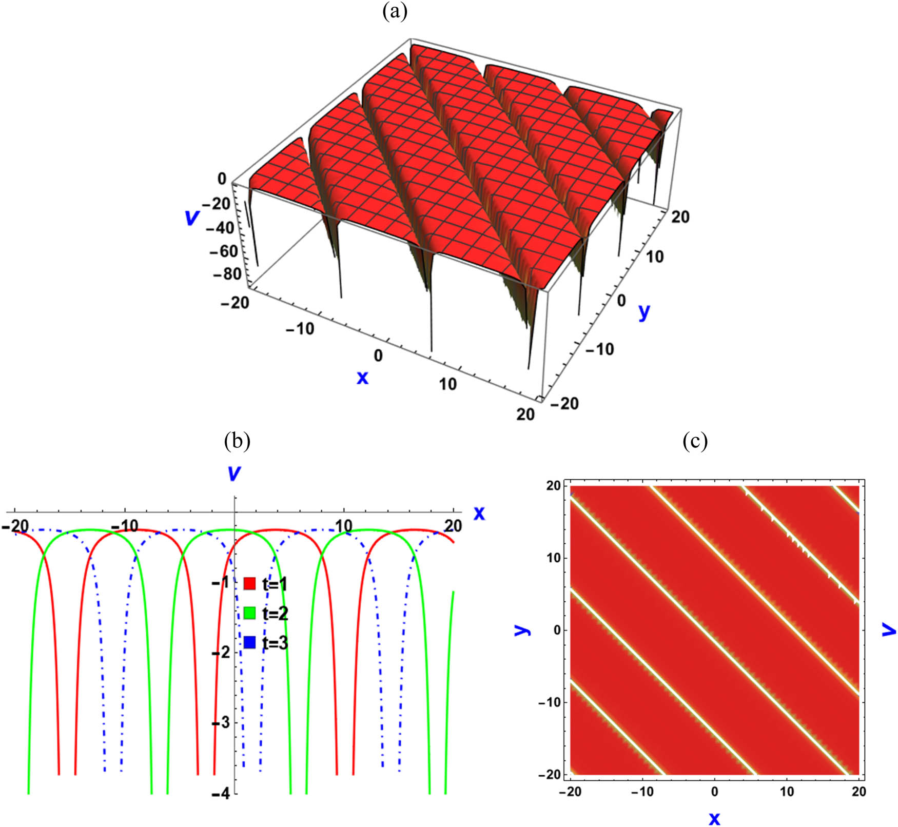
Visualizing the solution that consists of multi-singular solitons across different plots, where

Visualizing the solution that consists of V-type and bell-type solitons across different plots, where

Visualizing the solution that consists of parabolic solitons across different plots, where
Visualizing the solution that consists of periodic singular solitons across different plots, where

Visualizing the solution that consists of Kuznetsov–Ma Breather solitons across different plots, where

Visualizing the solution that consists of complex multi-singular solitons across different plots, where

Visualizing the solution that consists of dark-type kink solitons across different plots, where
The solutions derived from Eq. (3) display a variety of forms, including the multi-singular soliton, V-type and bell-type soliton, parabolic soliton, periodic singular soliton, Kuznetsov–Ma Breather soliton, complex multi-singular soliton, and kink-like soliton. These diverse forms of solitons find broad applications across scientific and engineering disciplines. The multi-singular soliton plays a key role in studying wave interactions in nonlinear systems, applicable from optics to plasma physics. V-type and bell solitons are essential in optical communications for their ability to maintain stable waveforms, ensuring reliable data transmission over long distances. Parabolic solitons are significant in fluid dynamics, where they model shallow water waves and predict surface disturbances in natural water bodies. In nonlinear optics, periodic singular solitons are crucial for examining periodic disturbances in electromagnetic fields. Kuznetsov–Ma Breather solitons find practical use in plasma physics and oceanography, providing insights into periodic oscillations and wave behaviors. Complex multi-singular solitons are employed in condensed matter physics to explore intricate interactions in materials science. Kink-like solitons are fundamental in field theory and nonlinear optics, offering insights into phase transitions and dynamics of domain walls in various materials. These solitons contribute significantly to advancing our understanding of nonlinear phenomena and driving innovations across diverse scientific and technological domains.
6 Comparison
This section underscores the originality and scientific insights of our study by judging our results with those reported by Ali et al., Arnous et al., and Alqahtani and Kaplan [8,10,11]. The difference is keenly divided into two parts, examining both the resemblances and variations between our research methodologies. By clarifying these aspects, we aim to offer a comprehensive view of the new understanding provided to the field.
6.1 Equalities
All of the studies focus on the extended Sakovich equation, an essential model used to investigate solitary wave solutions.
All of the studies aim to derive exact solutions through analytical methods.
6.2 Variations and uniqueness
Other studies have employed various methods, such as the exp (−ψ(η)) expansion technique, the
Although previous research primarily concentrated on identifying various types of solitons, such as multiple singular, singular, dark, bright, and periodic solitons, our study broadens this scope to include a more diverse range of solitons. This includes singular, multi-singular, periodic singular, kink, anti-kink, bell-shaped, Kuznetsov–Ma Breather, and parabolic-shaped solitons. Among these, the periodic singular, bell-shaped, Kuznetsov–Ma Breather, and parabolic-shaped solitons introduced in our research represent significant and novel contributions within this equation.
Furthermore, this study performs bifurcation and modulation instability analyses on the equation. The bifurcation analysis provides insights into the phase portrait, while the modulation instability analysis reveals stable dispersion during wave propagation. These analyses offer unique contributions, as they are not typically included in similar studies.
7 Conclusions
This study focused on the extended Sakovich equation, emphasizing the crucial role of soliton solutions in predicting and controlling localized wave behaviors, thereby advancing nonlinear dynamics and related applications. Effective bifurcation analysis confirmed the saddle point and center point behaviors within the equation’s phase portrait. Modulation instability analyses revealed a stable dispersion pattern for this equation. The improved Sardar subequation method and the
Acknowledgments
The authors would like to acknowledge the Deanship of Graduate Studies and Scientific Research, Taif University for funding this work.
-
Funding information: The authors would like to acknowledge the Deanship of Graduate Studies and Scientific Research, Taif University for funding this work.
-
Author contributions: All authors have accepted responsibility for the entire content of this manuscript and approved its submission.
-
Conflict of interest: The authors state no conflict of interest.
-
Data availability statement: All data generated or analyzed during this study are included in this published article.
References
[1] Jafari H, Kadkhoda N, Baleanu D. Fractional Lie group method of the time-fractional Boussinesq equation. Nonlinear Dyn. 2015;81:1569–74. 10.1007/s11071-015-2091-4.Suche in Google Scholar
[2] Hossain MN, Miah MM, Hamid A, Osman GMS. Discovering new abundant optical solutions for the resonant nonlinear Schrödinger equation using an analytical technique. Opt Quantum Electron. 2024;56:847. 10.1007/s11082-024-06351-5.Suche in Google Scholar
[3] Bilal M, Seadawy AR, Younis M, Rizvi STR, El-Rashidy K, Mahmoud SF. Analytical wave structures in plasma physics modelled by Gilson-Pickering equation by two integration norms. Results Phys. 2021;23:103959. 10.1016/j.rinp.2021.103959.Suche in Google Scholar
[4] Liu JG, Osman MS, Zhu WH, Zhou L, Ai GP. Different complex wave structures described by the Hirota Equation with variable coefficients in inhomogeneous optical fibers. Appl Phys B Lasers Opt. 2019;125:1–9. 10.1007/s00340-019-7287-8.Suche in Google Scholar
[5] Zhu C, Al-Dossari M, Rezapour S, Shateyi S, Gunay B. Analytical optical solutions to the nonlinear Zakharov system via logarithmic transformation. Results Phys. 2024;56:107298. 10.1016/j.rinp.2023.107298.Suche in Google Scholar
[6] Hamid I, Kumar S. Symbolic computation and Novel solitons, traveling waves and soliton-like solutions for the highly nonlinear (2 + 1)-dimensional Schrödinger equation in the anomalous dispersion regime via newly proposed modified approach. Opt Quantum Electron. 2023;55(9):755. 10.1007/s11082-023-04903-9.Suche in Google Scholar
[7] Kai Y, Yin Z. Linear structure and soliton molecules of Sharma-Tasso-Olver-Burgers equation. Phys Lett A. 2022;452:128430. 10.1016/j.physleta.2022.128430.Suche in Google Scholar
[8] Ali KK, AlQahtani SA, Mehanna MS, Wazwaz AM. Novel soliton solutions for the (3 + 1)-dimensional Sakovich equation using different analytical methods. J Math. 2023;2023:4864334. 10.1155/2023/4864334.Suche in Google Scholar
[9] Younis M, Seadawy AR, Baber MZ, Yasin MW, Rizvi STR, Iqbal MS. Abundant solitary wave structures of the higher dimensional Sakovich dynamical model. Math Methods Appl Sci. 2021;1–18. 10.1002/mma.7919.Suche in Google Scholar
[10] Arnous AH, Hashemi MS, Nisar KS, Shakeel M, Ahmad J, Ahmad I, et al. Investigating solitary wave solutions with enhanced algebraic method for new extended Sakovich equations in fluid dynamics. Results Phys. 2024;57:107369. 10.1016/j.rinp.2024.107369.Suche in Google Scholar
[11] Alqahtani RT, Kaplan M. Analyzing soliton solutions of the extended (3 + 1)-dimensional Sakovich equation. Mathematics. 2024;12:1–10. 10.3390/math12050720.Suche in Google Scholar
[12] Sakovich S. A new Painlevé-integrable equation possessing Kdv-type solitons. Nonlinear Phenom Complex Syst. 2019;22:299–304, https://arxiv.org/abs/1907.01324.Suche in Google Scholar
[13] Wazwaz A-M. A new (3 + 1)-dimensional Painlevé-integrable Sakovich equation: multiple soliton solutions. Int J Numer Methods Heat Fluid Flow. 2021;31:3030–5. 10.1108/HFF-11-2020-0687.Suche in Google Scholar
[14] Kumar S, Rani S, Mann N. Diverse analytical wave solutions and dynamical behaviors of the new (2 + 1)-dimensional Sakovich equation emerging in fluid dynamics. Eur Phys J Plus. 2022;137(11):1226. 10.1140/epjp/s13360-022-03397-w.Suche in Google Scholar
[15] Ma Y-L, Wazwaz A-M, Li B-Q. A new (3 + 1)-dimensional Sakovich equation in nonlinear wave motion: Painlevé integrability, multiple solitons and soliton molecules. Qual Theory Dyn Syst. 2022;21:158. 10.1007/s12346-022-00689-5.Suche in Google Scholar
[16] Kawser MA, Ali Akbar M, Khan MA, Ghazwan HA. Exact soliton solutions and the signifcance of time‑dependent coefcients in the Boussinesq equation: theory and application in mathematical physics. Sci Rep. 2024;14:762. 10.1038/s41598-023-50782-1.Suche in Google Scholar PubMed PubMed Central
[17] Mann N, Rani S, Kumar S, Kumar R. Novel closed-form analytical solutions and modulation instability spectrum induced by the Salerno equation describing nonlinear discrete electrical lattice via symbolic computation. Math Comput Simul. 2024;219:473–90. 10.1016/j.matcom.2023.12.031.Suche in Google Scholar
[18] Borhan JRM, Ganie AH, Miah MM, Iqbal MA, Seadawy AR, Mishra NK. A highly effective analytical approach to innovate the novel closed form soliton solutions of the Kadomtsev–Petviashivili equations with applications. Opt Quantum Electron. 2024;56:1–23. 10.1007/s11082-024-06706-y.Suche in Google Scholar
[19] Iqbal MA, Miah MM, Rasid MM, Alshehri HM, Osman MS. An investigation of two integro-differential KP hierarchy equations to find out closed form solitons in mathematical physics. Arab J Basic Appl Sci. 2023;30:535–45. 10.1080/25765299.2023.2256049.Suche in Google Scholar
[20] Ma WX. N-soliton solutions and the Hirota conditions in (1 + 1)-dimensions. Int J Nonlinear Sci Numer Simul. 2022;23:123–33. 10.1515/ijnsns-2020-0214.Suche in Google Scholar
[21] Gu Y, Manafian J, Malmir S, Eslami B, Ilhan OA. Lump, lump-trigonometric, breather waves, periodic wave and multi-waves solutions for a Konopelchenko–Dubrovsky equation arising in fluid dynamics. Int J Mod Phys B. 2023 Jun;37(15):2350141. 10.1142/S0217979223501412.Suche in Google Scholar
[22] Yomba E. The general projective Riccati equations method and exact solutions for a class of nonlinear partial differential equations. Chin J Phys. 2005;43:991–1003, https://www.airitilibrary.com/Article/Detail?DocID=05779073-200512-201210080016-201210080016-991-1003.Suche in Google Scholar
[23] Mann N, Kumar S, Ma WX. Dynamics of analytical solutions and Soliton-like profiles for the nonlinear complex-coupled Higgs field equation. Partial Differ Equ Appl Math. 2024;10:100733. 10.1016/j.padiff.2024.100733.Suche in Google Scholar
[24] Zafar A, Raheel M, Ali KK, Razzaq W. On optical soliton solutions of new Hamiltonian amplitude equation via Jacobi elliptic functions. Eur Phys J Plus. 2020;135:1–17. 10.1140/epjp/s13360-020-00694-0.Suche in Google Scholar
[25] Kai Y, Ji J, Yin Z. Study of the generalization of regularized long-wave equation. Nonlinear Dyn. 2022;107(3):2745–52. 10.1007/s11071-021-07115-6.Suche in Google Scholar
[26] Khan MAU, Akram G, Sadaf M. Dynamics of novel exact soliton solutions of concatenation model using efective techniques. Opt Quantum Electron. 2024;56:385. 10.1007/s11082-023-05957-5.Suche in Google Scholar
[27] Altawallbeh Z, Az-Zo’bi E, Alleddawi AO, Şenol M, Akinyemi L. Novel liquid crystals model and its nematicons. Opt Quant Electron. 2022;54:861. 10.1007/s11082-022-04279-2.Suche in Google Scholar
[28] Babajanov B, Abdikarimov F. The application of the functional variable method for solving the loaded non-linear evaluation equations. Front Appl Math Stat. 2022;8:1–9. 10.3389/fams.2022.912674.Suche in Google Scholar
[29] Ma WX, Zhu Z. Solving the (3 + 1)-dimensional generalized KP and BKP equations by the multiple exp-function algorithm. Appl Math Comput. 2012;218:11871–9. 10.1016/j.amc.2012.05.049.Suche in Google Scholar
[30] Kumar S, Dhiman SK. Exploring cone-shaped solitons, breather, and lump-forms solutions using the lie symmetry method and unified approach to a coupled breaking soliton model. Phys Scr. 2024;99(2):025243. 10.1088/1402-4896/ad1d9e.Suche in Google Scholar
[31] Islam SMR, Arafat SMY, Wang H. Abundant closed-form wave solutions to the simplified modified Camassa-Holm equation. J Ocean Eng Sci. 2023;8:238–45. 10.1016/j.joes.2022.01.012.Suche in Google Scholar
[32] Fan E. Extended tanh-function method and its applications to nonlinear equations. Phys Lett A. 2000;277:212–8. 10.1016/S0375-9601(00)00725-8.Suche in Google Scholar
[33] Nofal TA. Simple equation method for nonlinear partial differential equations and its applications. J Egypt Math Soc. 2016;24:204–9. 10.1016/j.joems.2015.05.006.Suche in Google Scholar
[34] Kumar A, Pankaj RD. Tanh–coth scheme for traveling wave solutions for nonlinear wave interaction model. J Egypt Math Soc. 2015;23:282–5. 10.1016/j.joems.2014.05.002.Suche in Google Scholar
[35] Habib MA, Ali HMS, Miah MM, Akbar MA. The generalized Kudryashov method for new closed form traveling wave solutions to some NLEEs. AIMS Math. 2019;4:896–909. 10.3934/math.2019.3.896.Suche in Google Scholar
[36] Fokas AS, Lenells J. The unified method: I. Nonlinearizable problems on the half-line. J Phys A Math Theor. 2012;45:195201. 10.1088/1751-8113/45/19/195201.Suche in Google Scholar
[37] Gu Y, Aminakbari N. New optical soliton solutions for the variable coefficients nonlinear Schrödinger equation. Opt Quant Electron. 2022;54:255. 10.1007/s11082-022-03645-4.Suche in Google Scholar
[38] Gu Y, Amin Akbari N. Bernoulli (G′/G)-expansion method for nonlinear Schrödinger equation with third-order dispersion. Mod Phys Lett B. 2022;36:2250028. 10.1142/S0217984922500282.Suche in Google Scholar
[39] Inc M, Az-Zo’bi EA, Jhangeer A, Rezazadeh H, Nasir A, Mohammed KA. New soliton solutions for the higher-dimensional non-local Ito equation. Nonlinear Eng. 2021;10(1):374–84. 10.1515/nleng-2021-0029.Suche in Google Scholar
[40] Rehman HU, Habib A, Ali K, Awan AU. Study of Langmuir waves for Zakharov equation using Sardar sub-equation method. Int J Nonlinear Anal Appl. 2023;14:9–18.Suche in Google Scholar
[41] Yasin S, Khan A, Ahmad S, Osman MS. New exact solutions of (3 + 1)-dimensional modified KdV-Zakharov-Kuznetsov equation by Sardar-subequation method. Opt Quantum Electron. 2024;56:1–15. 10.1007/s11082-023-05558-2.Suche in Google Scholar
[42] Bilal M, Shafqat-Ur-Rehman, Ahmad J. Stability analysis and diverse nonlinear optical pluses of dynamical model in birefringent fibers without four-wave mixing. Opt Quantum Electron. 2022;54:1–24. 10.1007/s11082-022-03659-y.Suche in Google Scholar
[43] Ibrahim S, Ashir AM, Sabawi YA, Baleanu D. Realization of optical solitons from nonlinear Schrödinger equation using modified Sardar sub-equation technique. Opt Quantum Electron. 2023;55:1–15. 10.1007/s11082-023-04776-y.Suche in Google Scholar
[44] Cinar M, Secer A, Ozisik M, Bayram M. Derivation of optical solitons of dimensionless Fokas-Lenells equation with perturbation term using Sardar sub-equation method. Opt Quantum Electron. 2022;54:1–13. 10.1007/s11082-022-03819-0.Suche in Google Scholar
[45] Hossain MN, El-Rashidy K, Alsharif F, Kanan M, Ma W-X, Miah MM. New optical soliton solutions to the Biswas – Milovic equations with power law and parabolic law nonlinearity using the Sardar‑subequation method. Opt Quantum Electron. 2024;56:1163. 10.1007/s11082-024-07073-4.Suche in Google Scholar
[46] Sadaf M, Arshed S, Akram G. Exact soliton and solitary wave solutions to the Fokas system using two variables (G′/G ,1/G) -expansion technique and generalized projective Riccati equation method. Optik. 2022;268:169713. 10.1016/j.ijleo.2022.169713.Suche in Google Scholar
[47] Vivas-Cortez M, Akram G, Sadaf M, Arshed S, Rehan K, Farooq K. Traveling wave behavior of new (2 + 1)-dimensional combined KdV–MKdV equation. Results Phys. 2023;45:106244. 10.1016/j.rinp.2023.106244.Suche in Google Scholar
[48] Sirisubtawee S, Koonprasert S, Sungnul S. Some applications of the (G’/G, 1/G)-expansion method for finding exact traveling wave solutions of nonlinear fractional evolution equations. Symmetry (Basel). 2019;11:1–29. 10.3390/sym11080952.Suche in Google Scholar
[49] Hossain MN, Miah MM, Duraihem FZ, Rehman S, Ma W-X. Chaotic behavior, bifurcations, sensitivity analysis, and novel optical soliton solutions to the Hamiltonian amplitude equation in optical physics. Phys Scr. 2024;99:075231. 10.1088/1402-4896/ad52fd.Suche in Google Scholar
[50] Hossain MN, Alsharif F, Miah MM, Kanan M. Abundant new optical soliton solutions to the Biswas – Milovic equation with sensitivity analysis for optimization. Mathematics. 2024;12:1585. 10.3390/math12101585.Suche in Google Scholar
[51] Rezazadeh H, Inc M, Baleanu D. New solitary wave solutions for variants of (3 + 1)-dimensional Wazwaz-Benjamin-Bona-Mahony equations. Front Phys. 2020;8:1–11. 10.3389/fphy.2020.00332.Suche in Google Scholar
[52] Hossain MN, Miah MM, Alosaimi M, Alsharif F, Kanan M. Exploring novel soliton solutions to the time-fractional coupled Drinfel’ d – Sokolov – Wilson equation in industrial engineering using two efficient techniques. Fractal Fract. 2024;8:352. 10.3390/fractalfract8060352.Suche in Google Scholar
[53] Hossain MN, Miah MM, Abbas MS, El-Rashidy K, Borhan JRM, Kanan M. An analytical study of the Mikhailov–Novikov–Wang equation with stability and modulation instability analysis in industrial engineering via multiple methods. Symmetry. 2024;16:879. 10.3390/sym16070879.Suche in Google Scholar
[54] Rasid MM, Miah MM, Ganie AH, Alshehri HM, Osman MS, Ma WX. Further advanced investigation of the complex Hirota-dynamical model to extract soliton solutions. Mod Phys Lett B. 2023;2450074:1–18. 10.1142/S021798492450074X.Suche in Google Scholar
[55] Li LX, Li EQ, Wang ML. The (G′/G, 1/G)-expansion method and its application to travelling wave solutions of the Zakharov equations. Appl Math. 2010;25:454–62. 10.1007/s11766-010-2128-x.Suche in Google Scholar
[56] Rafiq MH, Raza N, Jhangeer A. Dynamic study of bifurcation, chaotic behavior and multi-soliton profiles for the system of shallow water wave equations with their stability. Chaos, Solitons Fractals. 2023;171:113436. 10.1016/j.chaos.2023.113436.Suche in Google Scholar
[57] Zhu C, Al-Dossari M, Rezapour S, Alsallami SA, Gunay B. Bifurcations, chaotic behavior, and optical solutions for the complex Ginzburg–Landau equation. Results Phys. 2024;59:107601. 10.1016/j.rinp.2024.107601.Suche in Google Scholar
[58] Younis M, Sulaiman TA, Bilal M, Rehman SU, Younas U. Modulation instability analysis, optical and other solutions to the modified nonlinear Schrödinger equation. Commun Theor Phys. 2020;72:065001. 10.1088/1572-9494/ab7ec8.Suche in Google Scholar
[59] Hossain MN, Miah MM, Duraihem FZ, Rehman S. Stability, modulation instability, and analytical study of the confirmable time fractional Westervelt equation and the Wazwaz Kaur Boussinesq equation. Opt Quantum Electron. 2024;56:1–29. 10.1007/s11082-024-06776-y.Suche in Google Scholar
[60] Rahman RU, Hammouch Z, Alsubaie AS, Mahmoud KH, Alshehri A, Az-Zo’bi EA, et al. Dynamical behavior of fractional nonlinear dispersive equation in Murnaghan’s rod materials. Results Phys. 2024 Jan;56:107207. 10.1016/j.rinp.2023.107207.Suche in Google Scholar
[61] Muhammad S, Abbas N, Hussain A, Az-Zo’bi E. Dynamical features and traveling wave structures of the perturbed Fokas-Lenells equation in nonlinear optical fibers. Phys Scr. 2024 Feb;99(3):035201. 10.1088/1402-4896/ad1fc7.Suche in Google Scholar
© 2024 the author(s), published by De Gruyter
This work is licensed under the Creative Commons Attribution 4.0 International License.
Artikel in diesem Heft
- Regular Articles
- Numerical study of flow and heat transfer in the channel of panel-type radiator with semi-detached inclined trapezoidal wing vortex generators
- Homogeneous–heterogeneous reactions in the colloidal investigation of Casson fluid
- High-speed mid-infrared Mach–Zehnder electro-optical modulators in lithium niobate thin film on sapphire
- Numerical analysis of dengue transmission model using Caputo–Fabrizio fractional derivative
- Mononuclear nanofluids undergoing convective heating across a stretching sheet and undergoing MHD flow in three dimensions: Potential industrial applications
- Heat transfer characteristics of cobalt ferrite nanoparticles scattered in sodium alginate-based non-Newtonian nanofluid over a stretching/shrinking horizontal plane surface
- The electrically conducting water-based nanofluid flow containing titanium and aluminum alloys over a rotating disk surface with nonlinear thermal radiation: A numerical analysis
- Growth, characterization, and anti-bacterial activity of l-methionine supplemented with sulphamic acid single crystals
- A numerical analysis of the blood-based Casson hybrid nanofluid flow past a convectively heated surface embedded in a porous medium
- Optoelectronic–thermomagnetic effect of a microelongated non-local rotating semiconductor heated by pulsed laser with varying thermal conductivity
- Thermal proficiency of magnetized and radiative cross-ternary hybrid nanofluid flow induced by a vertical cylinder
- Enhanced heat transfer and fluid motion in 3D nanofluid with anisotropic slip and magnetic field
- Numerical analysis of thermophoretic particle deposition on 3D Casson nanofluid: Artificial neural networks-based Levenberg–Marquardt algorithm
- Analyzing fuzzy fractional Degasperis–Procesi and Camassa–Holm equations with the Atangana–Baleanu operator
- Bayesian estimation of equipment reliability with normal-type life distribution based on multiple batch tests
- Chaotic control problem of BEC system based on Hartree–Fock mean field theory
- Optimized framework numerical solution for swirling hybrid nanofluid flow with silver/gold nanoparticles on a stretching cylinder with heat source/sink and reactive agents
- Stability analysis and numerical results for some schemes discretising 2D nonconstant coefficient advection–diffusion equations
- Convective flow of a magnetohydrodynamic second-grade fluid past a stretching surface with Cattaneo–Christov heat and mass flux model
- Analysis of the heat transfer enhancement in water-based micropolar hybrid nanofluid flow over a vertical flat surface
- Microscopic seepage simulation of gas and water in shale pores and slits based on VOF
- Model of conversion of flow from confined to unconfined aquifers with stochastic approach
- Study of fractional variable-order lymphatic filariasis infection model
- Soliton, quasi-soliton, and their interaction solutions of a nonlinear (2 + 1)-dimensional ZK–mZK–BBM equation for gravity waves
- Application of conserved quantities using the formal Lagrangian of a nonlinear integro partial differential equation through optimal system of one-dimensional subalgebras in physics and engineering
- Nonlinear fractional-order differential equations: New closed-form traveling-wave solutions
- Sixth-kind Chebyshev polynomials technique to numerically treat the dissipative viscoelastic fluid flow in the rheology of Cattaneo–Christov model
- Some transforms, Riemann–Liouville fractional operators, and applications of newly extended M–L (p, s, k) function
- Magnetohydrodynamic water-based hybrid nanofluid flow comprising diamond and copper nanoparticles on a stretching sheet with slips constraints
- Super-resolution reconstruction method of the optical synthetic aperture image using generative adversarial network
- A two-stage framework for predicting the remaining useful life of bearings
- Influence of variable fluid properties on mixed convective Darcy–Forchheimer flow relation over a surface with Soret and Dufour spectacle
- Inclined surface mixed convection flow of viscous fluid with porous medium and Soret effects
- Exact solutions to vorticity of the fractional nonuniform Poiseuille flows
- In silico modified UV spectrophotometric approaches to resolve overlapped spectra for quality control of rosuvastatin and teneligliptin formulation
- Numerical simulations for fractional Hirota–Satsuma coupled Korteweg–de Vries systems
- Substituent effect on the electronic and optical properties of newly designed pyrrole derivatives using density functional theory
- A comparative analysis of shielding effectiveness in glass and concrete containers
- Numerical analysis of the MHD Williamson nanofluid flow over a nonlinear stretching sheet through a Darcy porous medium: Modeling and simulation
- Analytical and numerical investigation for viscoelastic fluid with heat transfer analysis during rollover-web coating phenomena
- Influence of variable viscosity on existing sheet thickness in the calendering of non-isothermal viscoelastic materials
- Analysis of nonlinear fractional-order Fisher equation using two reliable techniques
- Comparison of plan quality and robustness using VMAT and IMRT for breast cancer
- Radiative nanofluid flow over a slender stretching Riga plate under the impact of exponential heat source/sink
- Numerical investigation of acoustic streaming vortices in cylindrical tube arrays
- Numerical study of blood-based MHD tangent hyperbolic hybrid nanofluid flow over a permeable stretching sheet with variable thermal conductivity and cross-diffusion
- Fractional view analytical analysis of generalized regularized long wave equation
- Dynamic simulation of non-Newtonian boundary layer flow: An enhanced exponential time integrator approach with spatially and temporally variable heat sources
- Inclined magnetized infinite shear rate viscosity of non-Newtonian tetra hybrid nanofluid in stenosed artery with non-uniform heat sink/source
- Estimation of monotone α-quantile of past lifetime function with application
- Numerical simulation for the slip impacts on the radiative nanofluid flow over a stretched surface with nonuniform heat generation and viscous dissipation
- Study of fractional telegraph equation via Shehu homotopy perturbation method
- An investigation into the impact of thermal radiation and chemical reactions on the flow through porous media of a Casson hybrid nanofluid including unstable mixed convection with stretched sheet in the presence of thermophoresis and Brownian motion
- Establishing breather and N-soliton solutions for conformable Klein–Gordon equation
- An electro-optic half subtractor from a silicon-based hybrid surface plasmon polariton waveguide
- CFD analysis of particle shape and Reynolds number on heat transfer characteristics of nanofluid in heated tube
- Abundant exact traveling wave solutions and modulation instability analysis to the generalized Hirota–Satsuma–Ito equation
- A short report on a probability-based interpretation of quantum mechanics
- Study on cavitation and pulsation characteristics of a novel rotor-radial groove hydrodynamic cavitation reactor
- Optimizing heat transport in a permeable cavity with an isothermal solid block: Influence of nanoparticles volume fraction and wall velocity ratio
- Linear instability of the vertical throughflow in a porous layer saturated by a power-law fluid with variable gravity effect
- Thermal analysis of generalized Cattaneo–Christov theories in Burgers nanofluid in the presence of thermo-diffusion effects and variable thermal conductivity
- A new benchmark for camouflaged object detection: RGB-D camouflaged object detection dataset
- Effect of electron temperature and concentration on production of hydroxyl radical and nitric oxide in atmospheric pressure low-temperature helium plasma jet: Swarm analysis and global model investigation
- Double diffusion convection of Maxwell–Cattaneo fluids in a vertical slot
- Thermal analysis of extended surfaces using deep neural networks
- Steady-state thermodynamic process in multilayered heterogeneous cylinder
- Multiresponse optimisation and process capability analysis of chemical vapour jet machining for the acrylonitrile butadiene styrene polymer: Unveiling the morphology
- Modeling monkeypox virus transmission: Stability analysis and comparison of analytical techniques
- Fourier spectral method for the fractional-in-space coupled Whitham–Broer–Kaup equations on unbounded domain
- The chaotic behavior and traveling wave solutions of the conformable extended Korteweg–de-Vries model
- Research on optimization of combustor liner structure based on arc-shaped slot hole
- Construction of M-shaped solitons for a modified regularized long-wave equation via Hirota's bilinear method
- Effectiveness of microwave ablation using two simultaneous antennas for liver malignancy treatment
- Discussion on optical solitons, sensitivity and qualitative analysis to a fractional model of ion sound and Langmuir waves with Atangana Baleanu derivatives
- Reliability of two-dimensional steady magnetized Jeffery fluid over shrinking sheet with chemical effect
- Generalized model of thermoelasticity associated with fractional time-derivative operators and its applications to non-simple elastic materials
- Migration of two rigid spheres translating within an infinite couple stress fluid under the impact of magnetic field
- A comparative investigation of neutron and gamma radiation interaction properties of zircaloy-2 and zircaloy-4 with consideration of mechanical properties
- New optical stochastic solutions for the Schrödinger equation with multiplicative Wiener process/random variable coefficients using two different methods
- Physical aspects of quantile residual lifetime sequence
- Synthesis, structure, I–V characteristics, and optical properties of chromium oxide thin films for optoelectronic applications
- Smart mathematically filtered UV spectroscopic methods for quality assurance of rosuvastatin and valsartan from formulation
- A novel investigation into time-fractional multi-dimensional Navier–Stokes equations within Aboodh transform
- Homotopic dynamic solution of hydrodynamic nonlinear natural convection containing superhydrophobicity and isothermally heated parallel plate with hybrid nanoparticles
- A novel tetra hybrid bio-nanofluid model with stenosed artery
- Propagation of traveling wave solution of the strain wave equation in microcrystalline materials
- Innovative analysis to the time-fractional q-deformed tanh-Gordon equation via modified double Laplace transform method
- A new investigation of the extended Sakovich equation for abundant soliton solution in industrial engineering via two efficient techniques
- New soliton solutions of the conformable time fractional Drinfel'd–Sokolov–Wilson equation based on the complete discriminant system method
- Irradiation of hydrophilic acrylic intraocular lenses by a 365 nm UV lamp
- Inflation and the principle of equivalence
- The use of a supercontinuum light source for the characterization of passive fiber optic components
- Optical solitons to the fractional Kundu–Mukherjee–Naskar equation with time-dependent coefficients
- A promising photocathode for green hydrogen generation from sanitation water without external sacrificing agent: silver-silver oxide/poly(1H-pyrrole) dendritic nanocomposite seeded on poly-1H pyrrole film
- Photon balance in the fiber laser model
- Propagation of optical spatial solitons in nematic liquid crystals with quadruple power law of nonlinearity appears in fluid mechanics
- Theoretical investigation and sensitivity analysis of non-Newtonian fluid during roll coating process by response surface methodology
- Utilizing slip conditions on transport phenomena of heat energy with dust and tiny nanoparticles over a wedge
- Bismuthyl chloride/poly(m-toluidine) nanocomposite seeded on poly-1H pyrrole: Photocathode for green hydrogen generation
- Infrared thermography based fault diagnosis of diesel engines using convolutional neural network and image enhancement
- On some solitary wave solutions of the Estevez--Mansfield--Clarkson equation with conformable fractional derivatives in time
- Impact of permeability and fluid parameters in couple stress media on rotating eccentric spheres
- Review Article
- Transformer-based intelligent fault diagnosis methods of mechanical equipment: A survey
- Special Issue on Predicting pattern alterations in nature - Part II
- A comparative study of Bagley–Torvik equation under nonsingular kernel derivatives using Weeks method
- On the existence and numerical simulation of Cholera epidemic model
- Numerical solutions of generalized Atangana–Baleanu time-fractional FitzHugh–Nagumo equation using cubic B-spline functions
- Dynamic properties of the multimalware attacks in wireless sensor networks: Fractional derivative analysis of wireless sensor networks
- Prediction of COVID-19 spread with models in different patterns: A case study of Russia
- Study of chronic myeloid leukemia with T-cell under fractal-fractional order model
- Accumulation process in the environment for a generalized mass transport system
- Analysis of a generalized proportional fractional stochastic differential equation incorporating Carathéodory's approximation and applications
- Special Issue on Nanomaterial utilization and structural optimization - Part II
- Numerical study on flow and heat transfer performance of a spiral-wound heat exchanger for natural gas
- Study of ultrasonic influence on heat transfer and resistance performance of round tube with twisted belt
- Numerical study on bionic airfoil fins used in printed circuit plate heat exchanger
- Improving heat transfer efficiency via optimization and sensitivity assessment in hybrid nanofluid flow with variable magnetism using the Yamada–Ota model
- Special Issue on Nanofluids: Synthesis, Characterization, and Applications
- Exact solutions of a class of generalized nanofluidic models
- Stability enhancement of Al2O3, ZnO, and TiO2 binary nanofluids for heat transfer applications
- Thermal transport energy performance on tangent hyperbolic hybrid nanofluids and their implementation in concentrated solar aircraft wings
- Studying nonlinear vibration analysis of nanoelectro-mechanical resonators via analytical computational method
- Numerical analysis of non-linear radiative Casson fluids containing CNTs having length and radius over permeable moving plate
- Two-phase numerical simulation of thermal and solutal transport exploration of a non-Newtonian nanomaterial flow past a stretching surface with chemical reaction
- Natural convection and flow patterns of Cu–water nanofluids in hexagonal cavity: A novel thermal case study
- Solitonic solutions and study of nonlinear wave dynamics in a Murnaghan hyperelastic circular pipe
- Comparative study of couple stress fluid flow using OHAM and NIM
- Utilization of OHAM to investigate entropy generation with a temperature-dependent thermal conductivity model in hybrid nanofluid using the radiation phenomenon
- Slip effects on magnetized radiatively hybridized ferrofluid flow with acute magnetic force over shrinking/stretching surface
- Significance of 3D rectangular closed domain filled with charged particles and nanoparticles engaging finite element methodology
- Robustness and dynamical features of fractional difference spacecraft model with Mittag–Leffler stability
- Characterizing magnetohydrodynamic effects on developed nanofluid flow in an obstructed vertical duct under constant pressure gradient
- Study on dynamic and static tensile and puncture-resistant mechanical properties of impregnated STF multi-dimensional structure Kevlar fiber reinforced composites
- Thermosolutal Marangoni convective flow of MHD tangent hyperbolic hybrid nanofluids with elastic deformation and heat source
- Investigation of convective heat transport in a Carreau hybrid nanofluid between two stretchable rotatory disks
- Single-channel cooling system design by using perforated porous insert and modeling with POD for double conductive panel
- Special Issue on Fundamental Physics from Atoms to Cosmos - Part I
- Pulsed excitation of a quantum oscillator: A model accounting for damping
- Review of recent analytical advances in the spectroscopy of hydrogenic lines in plasmas
- Heavy mesons mass spectroscopy under a spin-dependent Cornell potential within the framework of the spinless Salpeter equation
- Coherent manipulation of bright and dark solitons of reflection and transmission pulses through sodium atomic medium
- Effect of the gravitational field strength on the rate of chemical reactions
- The kinetic relativity theory – hiding in plain sight
- Special Issue on Advanced Energy Materials - Part III
- Eco-friendly graphitic carbon nitride–poly(1H pyrrole) nanocomposite: A photocathode for green hydrogen production, paving the way for commercial applications