Geometric nonlinear analysis based on the generalized displacement control method and orthogonal iteration

2.1 GDC method for nonlinear geometric elements

In nonlinear analysis, incremental theory is used to gradually solve the response of structures under nonlinear forces (such as material nonlinearity, geometric nonlinearity, etc.). When applying the incremental theory for nonlinear analysis, it is necessary to decompose the loading process of the structure into multiple equilibrium states for step-by-step analysis, as shown in Figure 1.

Figure 1

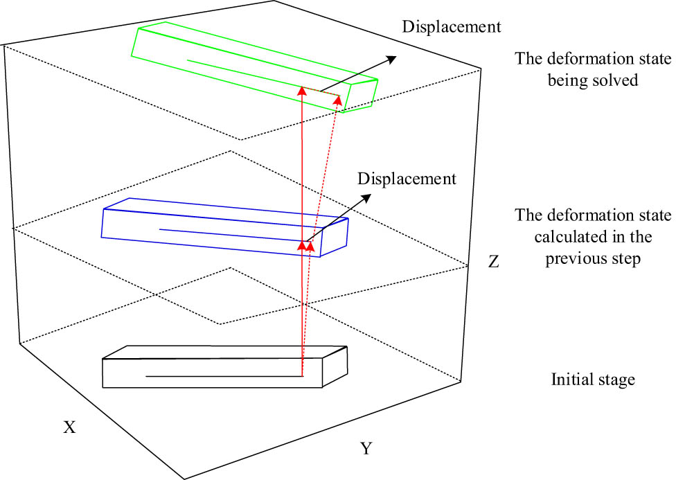
Deformation of building structural units in three-dimensional space.

As shown in Figure 1, the loading process is usually divided into three stages: the initial state, the deformation state calculated in the previous step, and the deformation state currently being solved. The initial state and the deformation state calculated in the previous step are known as equilibrium states, and a new equilibrium state is solved by analyzing the known equilibrium states [14]. Incremental stiffness can be calculated from the four parameters of structural displacement, elastic stiffness, geometric stiffness, and the force that generates displacement. The state changes of non-linear geometric structures are decomposed into linear problems through incremental stiffness, and the convergence of calculation errors is achieved through iterative increments. In the linear iteration process, the incremental equilibrium equation is expressed as:

In Eq. (1), i represents the number of incremental steps; j represents the number of iteration steps. [ S j − 1 i ] represents the overall stiffness matrix of the j − 1 -th incremental step of the structure. Δ D represents the displacement increment in the iteration; L represents the vector formed by the node forces caused by external loads; F represents the vector formed by the node forces caused by internal loads. The parameter L is obtained by calculating the load vector and the load increment coefficient. The unbalanced force represented by { L j i } − { F j − 1 i } in Eq. (1) is a limiting condition for the number of incremental iterations. Therefore, Eq. (2) is rewritten as follows:

In Eq. (2), λ represents the load increment coefficient; L ˆ represents the initially set load vector; U represents the unbalanced force. Under the rigid body criterion, the initial displacement vector of the structure multiplied by the stiffness matrix equals the external load vector, while the displacement increment of the structure multiplied by the stiffness matrix equals the unbalanced force vector. Therefore, the calculation equation for the displacement increment can be derived, and the displacement equation for incremental steps can be obtained by iterating all displacement increments, as shown in Eq. (3)

According to the structural incremental equilibrium equation of Eq. (2), N equilibrium equations can be constructed, but there are N + 1 unknowns in the equations, namely N unknown displacement quantities and one load increment coefficient. Due to the presence of more unknowns than equations, an additional constraint equation needs to be introduced to solve this problem. The general form of the constraint equation is expressed as:

In Eq. (4), χ represents the parameter that determines the displacement change of the object; κ represents the parameter that determines the magnitude of the object load; C represents the limiting parameter of the object displacement system. T represents the transposition operation, which is used to swap the rows and columns of a vector or matrix. To obtain all unknowns, the constraint equation of Eq. (4) and the incremental equilibrium equation of Eq. (2) are combined to form the following equation:

In order for the iterative algorithm to converge to the correct solution, the constraint equation needs to satisfy the stability and boundedness conditions. To ensure the boundedness of load increment parameters and displacement increments, the determinant of the generalized stiffness matrix must be non-zero to avoid mathematical singularities. The expression for the determinant of the generalized stiffness matrix is shown in the following equation:

In Eq. (6), κ and ( χ ) T are both sub-terms of the stiffness matrix, so the load increment coefficient can be expressed as:

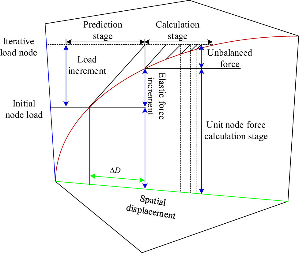
In the conventional incremental iteration method, it mainly includes the prediction stage that affects the speed and efficiency of algorithm convergence, as well as the calculation stage that directly determines whether the algorithm can converge to the exact solution, as shown in Figure 2.

Figure 2

Incremental iterative calculation model.

In Figure 2, when conducting nonlinear structural analysis, the incremental iterative calculation method needs to meet the requirement of automatically adjusting the step size to adapt to changes in structural stiffness [15]. Meanwhile, it is necessary to ensure stable calculation in areas where extreme values or rebound may occur. Therefore, the GDC method is introduced on the basis of incremental iterative calculation. The method uses the generalized stiffness parameter (GSP) to determine the size of the load increment and adjusts the iteration step size and loading/unloading directions in the iterative process to achieve the convergence of the solution [16]. Compared to other methods, it has advantages in dealing with complex nonlinear problems, dynamic problems, and material nonlinear problems with multiple critical points.

In the GDC method, the constraint parameters κ is 0, { χ } = λ 1 { Δ D ˆ 1 i − 1 } , C 1 = ( λ 1 1 ) 2 { Δ D ˆ 1 1 } T { Δ D 1 1 } , C j , j ≥ 2 = 0 . The constraint parameters are substituted into Eq. (7) to obtain the expression of the constraint equation, as shown in the following equation:

From Eq. (8), the calculation equation for the load increment coefficient can be simplified as:

In Eq. (9), PSG represents the generalized stiffness parameter. In the GDC method, both the stability at the limit point and rebound point, as well as the determination of loading and unloading directions during the iteration process, rely on GSP to achieve. GSP reflects the ratio of structural displacement increments and is numerically bounded and stable. The sign of GSP is related to the angle between the displacement increment [17]. When passing through extreme points, GSP is negative, while in other cases it is positive. The positive and negative values of GSP can be used to determine loading or unloading during the iteration process, helping the iteration process smoothly pass through the limit points. Therefore, the role of generalized stiffness parameters in nonlinear geometric problems is to adjust the value of the load increment parameter, thereby controlling the iteration step size.

When the number of iterations is greater than or equal to 2, the constraint Eq. (8) can be simplified into the following equation:

From Eq. (10), it can be seen that in the GDC iterative algorithm, the vector generated in the previous iteration is orthogonal to the vector generated in the current iteration. Therefore, the application of GSP can be used to ensure that the calculation of displacement changes of structures under load is carried out along new and unexplored directions, to avoid getting stuck in local minima or overfitting problems.

2.2 Improved GDC method based on orthogonal constraint conditions

The convergence of traditional incremental iteration methods depends on the initial guess value. If the initial conditions are not properly selected, it may lead to divergence or convergence to the wrong solution during the iteration process. Meanwhile, the efficiency and convergence of iterative methods may depend on the size and distribution of load increments. Since the orthogonal relationship between iterative increments has been analyzed in the above equation expression, the study aims to improve the GDC method by analyzing and optimizing the orthogonal constraint conditions. In incremental iteration analysis, the purpose of defining the load increment factor is to provide sufficient known conditions for solving the displacement and load increments in nonlinear equations. In the first iteration, it is assumed that the structure is in equilibrium and there are no unbalanced forces. At this stage, the structure is subjected to external loads, and the resulting displacement increment is calculated based on linear analysis. Starting from the second iteration, the iterative process gradually adjusts and optimizes to eliminate the unbalanced forces in the initial approximate solution, ultimately reaching an equilibrium state that makes the calculation results more accurate and reliable, as shown in Figure 3.

Figure 3

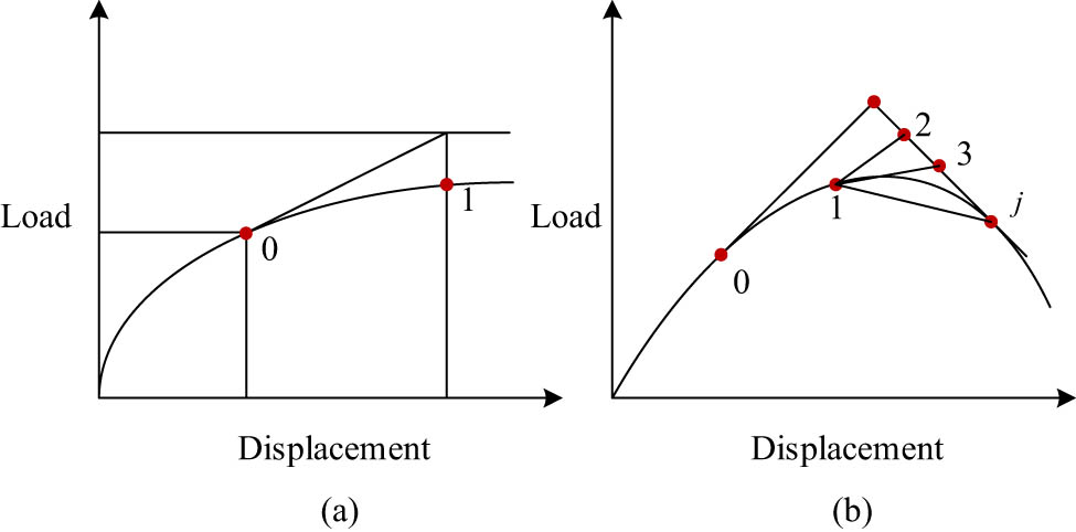
Two-dimensional simplification of traditional (a) incremental iteration and (b) generalized incremental orthogonal iteration.

In Figure 3, 0 represents the initial position, and 1, 2, 3, and j represent the number of iterations. In the first iteration, considering the degree of nonlinearity of the structure is crucial for determining the incremental step size. The stiffness change of a structure is an intuitive indicator for determining the degree of nonlinearity. A large change in stiffness means a high degree of nonlinearity, therefore requiring a smaller incremental step size. A small change in stiffness means a low degree of nonlinearity, and a larger incremental step size can be used. Therefore, the expression of the load increment coefficient should be optimized to the following equation:

In Eq. (11), f ( x ) is expressed as the correlation function of structural stiffness. Its expression is shown in the following equation:

In the first iteration of the incremental iteration method, in addition to determining the numerical value of the load increment coefficient, it is also necessary to determine its positive or negative sign. The current stiffness parameters used may not be sufficient to accurately describe the behavior of the structure near the limit point and rebound point, where special measures need to be taken to ensure the safety and stability of the structure. In practical applications, it is necessary to adjust the stiffness parameters or adopt more complex models to better handle these issues [18]. Therefore, the study introduces additional directional parameters to determine that when the dot product of two displacement increments is positive, the sign of the load increment coefficient is the same as that of the return parameter, as shown in the following equation:

In Eq. (13), sign represents the return parameter of the function, and when the dot product of two displacement increments is negative, it indicates that the sign of the load increment coefficient is opposite to that of the return parameter, as shown in the following equation:

In Eq. (14), λ 1 1 represents the preset value of the load increment coefficient, which is determined by the stiffness related function. In the initial iterative calculation, a simplified linear model obtains an approximate structural response of the nonlinear structure. The simplified linear calculation may lead to errors between the calculated results and the actual structural behavior. Therefore, the second part of the GDC method aims to reduce these errors through iteration. During the iteration process, a clear path or strategy needs to be defined to guide how to gradually adjust the load and displacement to approximate the true equilibrium state of the structure. The iteration path needs to be able to simultaneously adjust the load increment applied to the structure and the displacement increment of the structure. This adjustment is to gradually reduce the unbalanced state of the structure, so that the internal and external forces of the structure can reach equilibrium. In addition, the limit point and rebound point are nonlinear characteristic points in structural response. Inappropriate adjustment of the iteration path near these points can lead to divergence or inability to converge to the correct equilibrium state. The constraint equation of the current stiffness parameter method is simplified to Eq. (10), which shows that the current stiffness parameter uses orthogonal constraint conditions as its convergence criterion. Using the displacement increment within the incremental step as a reference direction vector can make the iteration direction closer to the equilibrium path. Therefore, the final GDC iteration path based on orthogonal constraint conditions is represented by the following equation:

Through this orthogonal iteration, the GDC method can effectively handle nonlinear problems in structural analysis. In structural analysis, a key parameter, the generalized stiffness parameter, is introduced to monitor the stiffness changes of the structure during loading. In the first step of iteration, the GDC method will set a step size limit to ensure the stability of the structure during loading and to determine whether to increase or decrease the load. In the subsequent steps of iteration, the GDC method will set a reference direction vector for the structure. This means that the iterative path of displacement increment will remain perpendicular to the reference direction vector, i.e., orthogonal, to ensure the efficiency and accuracy of the iterative process. Through the above iterative process, the goal of the GDC method is to stabilize and converge the calculation results to the equilibrium state of the structure. The research process is shown in Figure 4.

Figure 4

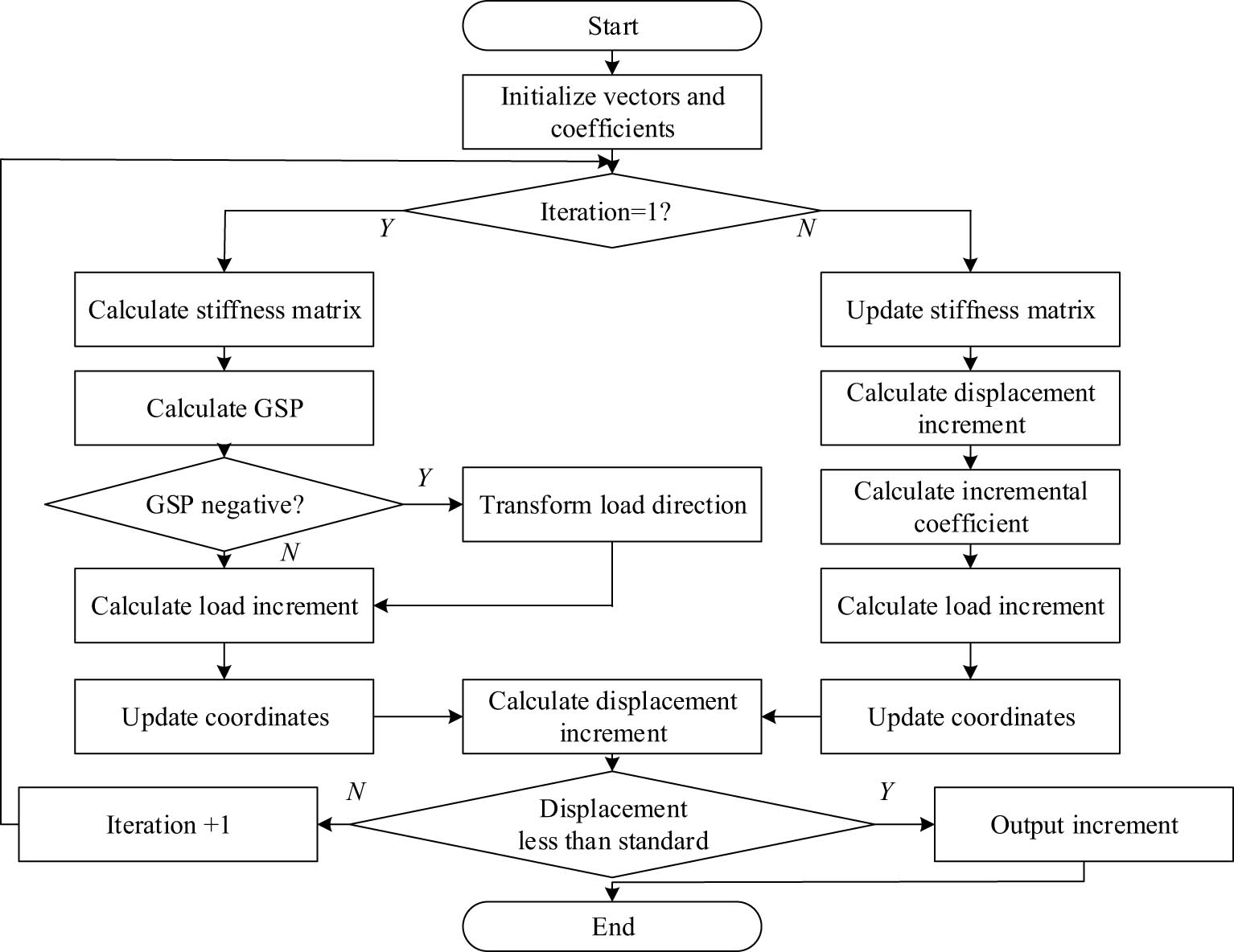
Algorithm flow based on GDC and incremental orthogonal iteration constraints.

In Figure 4, for the geometric nonlinearity problem of flexible structures, the GDC method and orthogonal constraints constructed by the research mainly divide the incremental iteration into two processes: the first iteration and the subsequent iteration.

In the first iteration, the stiffness matrix of the structure is determined and the GSP is calculated, and the positive and negative directions of the load are determined through the first iteration. The stiffness matrix of the second iteration is updated, and the load increment and displacement increment are calculated. Whether the displacement increment is less than the safety standard is judged. If yes, output the displacement increment; otherwise, continue iterative calculation. In the calculation and analysis of building structures, although traditional single displacement control methods are favored for their stability, they appear cumbersome when dealing with structural buckling problems. To ensure computational convergence when dealing with paths with significant curvature, it is usually necessary to set the initial load increment factor very small. In order to expand the application scope of displacement control iteration method, orthogonal constraint conditions are introduced to optimize the calculation process of the structure. By comparing the maximum load increment factor at convergence under different constraint conditions, the efficiency of structural analysis and calculation has been increased.

3.1 Applicability experiment of the orthogonal constraint optimization GDC method

The study uses a hexagonal star-shaped spatial truss structure as the experimental simulation object. When constructing a finite element analysis model using the ANSYS platform, LINK8 elements are used to construct the spatial truss structure, as shown in Figure 5.

Figure 5

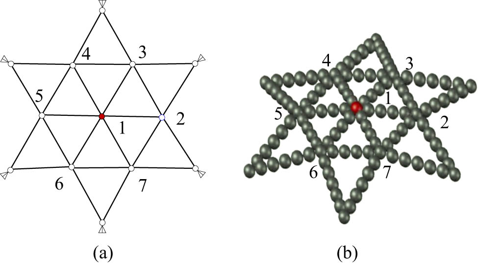
Model diagram and parallel simplification of the truss structure: (a) plan view and (b) discrete model diagram.

In Figure 5, in the finite element model constructed using ANSYS, each member is simplified into a single element for simulation. The contact relationship between each particle is simulated as 132 contact units, of which 48 contact points could rotate but are not allowed to translate at the connection. Additionally, 84 contact points allow for a certain degree of translation and rotation. The specific model parameters are shown in Table 1.

In the table, the initial load factor is used to determine the incremental step size and loading direction. The incremental step size should be adjusted according to the stiffness change of the structure, and the larger the stiffness, the smaller the incremental step size should be. Therefore, in order to reflect the changes in structural stiffness and adapt to the direction changes of loads beyond the limit point in iterative calculations, this value of 0.00005 is studied as the initial incremental coefficient. First, the load–displacement curve of the model is analyzed in the experiment to verify the rationality of the proposed orthogonal constraint optimization GDC method, as shown in Figure 6.

Figure 6

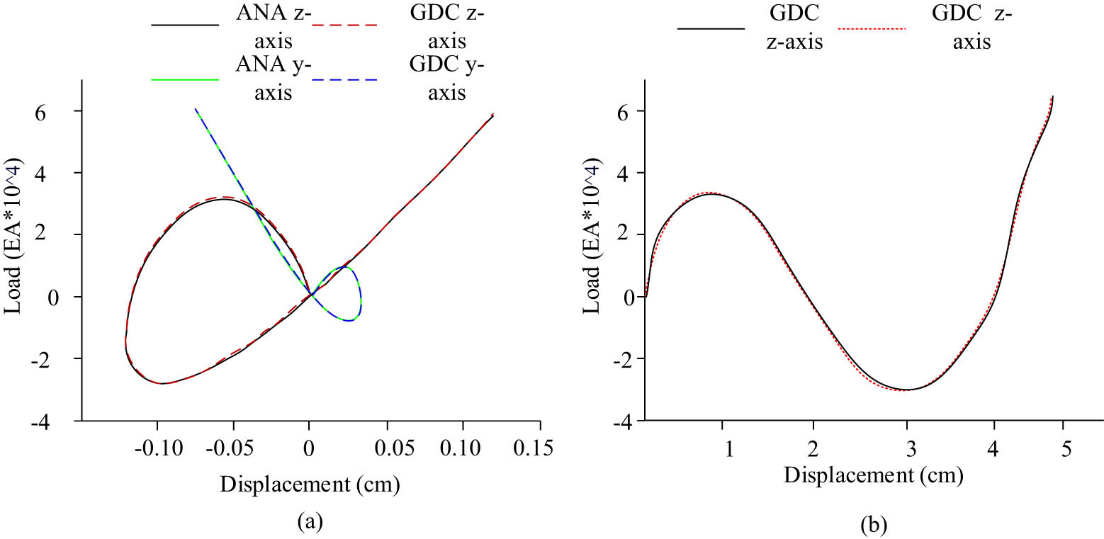
Node load–displacement curves using different methods: (a) Node 2 load displacement curve and (b) Node 1 load displacement curve.

In Figure 6, ANA represents the finite element analysis method, while GDC represents the analysis and calculation method constructed for the study. The proposed method is very close to the theoretical exact solution in the load–displacement curves of two nodes, indicating the accuracy of the analysis method. Experiments showed that the model constructed by the study could accurately predict and handle the performance of spatial frame structures when they reached their ultimate load-bearing capacity after introducing a stiffness matrix for analysis. Afterward, the study evaluates the efficiency of different methods, as shown in Figure 7.

Figure 7

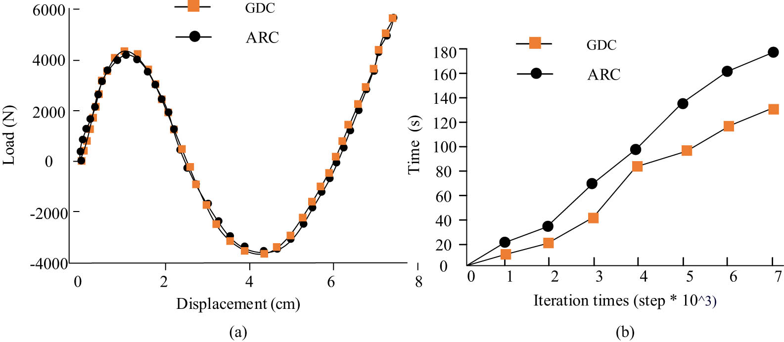
Load–displacement curves and calculation time of different methods: (a) Node 1 load displacement curve and (b) calculation time.

In Figure 7, ARC represents the cross-sectional method, while GDC represents the analytical calculation method constructed for the study. The method proposed in the study had similar load–displacement curves and section method curves, with a final time of 126 s in 700 incremental iteration steps, while the section method had a final time of 177 s. The method proposed in the study had optimized the time consumption by 28.8% compared to the cross-sectional method while maintaining the same performance.

3.2 Comparative experiment of the orthogonal constraint optimization GDC method

First, to analyze the computational performance of the model under different load conditions, the study will design different load conditions and analyze the performance of the orthogonal constraint optimized GDC method constructed under different loads in the calculation. First, the load is set to be uniformly applied from node 1. In the first working condition, the load method is to apply external loads directly, while in the second condition, the load is applied in a form greater than the external load. When the load of the second working condition exceeds that of the first working condition excessively, it will cause significant differences in nonlinear behavior. Therefore, the load of the second working condition in the study area is 1.01 times that of the first working condition. The load–displacement curves under two operating conditions are shown in Figure 8.

Figure 8

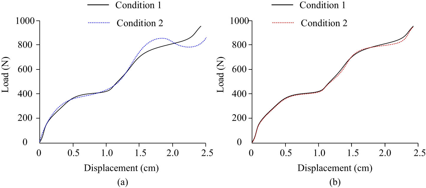
Load–displacement curves under different working conditions: (a) ARC load displacement curve and (b) GDC load displacement curve.

In Figure 8, under different operating conditions, the load–displacement curve of the cross-sectional method varied greatly, while the model constructed by the study is less affected by the change in operating conditions. From Figure 8(a), it can be seen that under the section method analysis, when the displacement of the contact element reaches 2.5 cm, the calculated load difference is as high as 97 N. In Figure 8(b), under the method of research construction, after the displacement of the method reaches 2.5 in the two working conditions, the load difference between different working conditions is only 4 N. To analyze and study the role of the proposed optimized GDC method in nonlinear structural deformation impact, a seismic wave with a peak acceleration of 1.2 g is input for 14 s in the simulation experiment. In the simulated disaster environment, the horizontal displacement of the simulated spatial truss structure is shown in Figure 9.

Figure 9

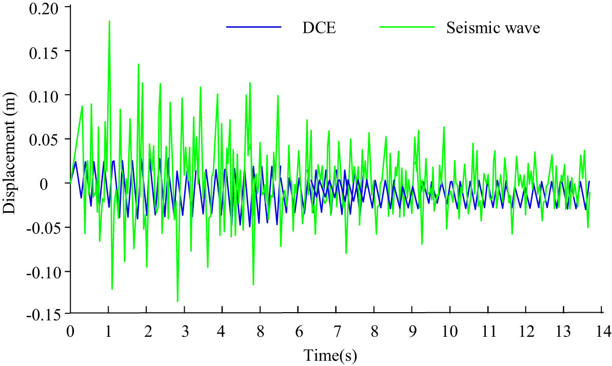
Horizontal displacement of spatial truss structures in simulated disaster environments.

The DEM in Figure 9 represents the discrete element analysis method. In Figure 9, the horizontal displacement results of the optimized GDC structure used in the study had a high similarity in waveform with the horizontal acceleration of seismic waves. The experiment showed that the N + 1 dimension theory used in the research method could effectively respond to and adjust the scope of application of the calculation method. The consistency and accuracy of calculation and analysis could also be maintained under the influence of geological disasters. The study analyzes the ultimate load fluctuations of contact elements in spatial truss structures under the influence of geological disasters, and the specific results are shown in Figure 10.

Figure 10

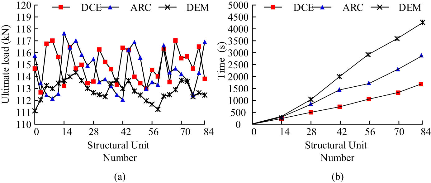
Ultimate load calculation and time consumption of contact elements in spatial truss structures: (a) structural critical load of different algorithms and (b) calculation time of different algorithms.

As shown in Figure 10, the difference in the ultimate load calculation of the contact element of the spatial truss structure between the algorithm models proposed by the three algorithms and the section method is relatively small, while the ultimate load obtained by the discrete element analysis method is larger compared to the other two methods. The average load calculation result of the discrete element analysis method for 84 contact elements is 112.6 kN, while the calculation results of the section method and the GDC method constructed in the study are 113.9 and 114.7 kN, respectively. In Figure 10(b), the constructed method took 1,615 s to calculate the ultimate load of 84 contact elements, while the cross-sectional method took 2,840 s to calculate all contact elements. The discrete element analysis method performed the worst in terms of computational efficiency, with a final computation time of 4,322 s. The time complexity of different algorithm models is shown in Figure 11.

Figure 11

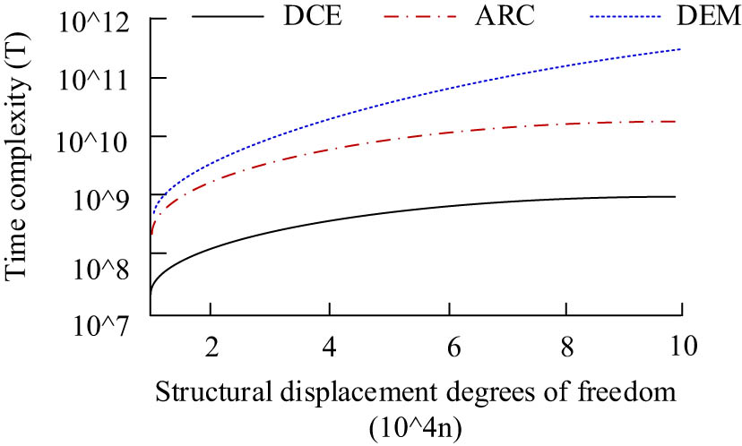
Time complexity of different algorithm models.

From Figure 11, it can be seen that with the increase of structural degrees of freedom, the time complexity of all three models shows an upward trend. However, the model constructed by the research has the smallest increase in magnitude, with a final time complexity of less than 10⁹ T, while the time service reading of the discrete element model is greater than 10¹¹ T, and the time complexity of the cross-sectional method is close to 10¹⁰ T. Afterward, the horizontal displacement and deformation degree of 13 nodes are compared in the study, and the specific results are shown in Table 2.

As observed in Table 2, among the 13 nodes, the maximum error of the constructed method in displacement calculation is only 0.06 cm, and the minimum error is 0 cm. Meanwhile, in all 13 nodes, the deformation judgment results calculated by the proposed method are correct. Therefore, the model constructed in the study can still accurately determine the displacement and deformation properties of building structures even after simulating earthquake disasters. Finally, the study will compare the differences between the GDC method, multi-point displacement control, and traditional LDL decomposition method constructed under different load conditions. In the comparative experiment, the three operating conditions are set as static overturning load, continuously increasing load, and reciprocating load. The specific results are shown in Table 3.

From Table 3, it can be seen that under the static overturning load conditions, the proposed algorithm has a time complexity of 0.52 × 10⁷ T, which is lower than other algorithm models. At the same time, under dynamic working conditions such as continuously increasing loads and reciprocating loads, the proposed algorithm has time complexities of 0.32 × 10⁸ T and 0.52 × 10⁷ T, respectively, which are lower than other algorithm models.

References

[1] Glass O, Kolumbán JJ, Sueur F. External boundary control of the motion of a rigid body immersed in a perfect two-dimensional fluid. Anal PDE. 2020;13(3):651–84.10.2140/apde.2020.13.651Suche in Google Scholar
[2] Coevoet E, Benchekroun O, Kry PG. Adaptive merging for rigid body simulation. ACM Trans Graphic (TOG). 2020;39(4):13–35.10.1145/3386569.3392417Suche in Google Scholar
[3] Touzé C, Vizzaccaro A, Thomas O. Model order reduction methods for geometrically nonlinear structures: a review of nonlinear techniques. Nonlinear Dyn. 2021;105(2):1141–90.10.1007/s11071-021-06693-9Suche in Google Scholar
[4] Deng J, Tan J, Tan P, Tian ZC. A geometric nonlinear plane beam element based on corotational formulation and on stability functions. Eng Mech. 2020;37(11):28–35.Suche in Google Scholar
[5] Ma Q, Grushin AG, Burch KS. Topology and geometry under the nonlinear electromagnetic spotlight. Nat Mater. 2021;20(12):1601–14.10.1038/s41563-021-00992-7Suche in Google Scholar
[6] Xu M, Zeng B, Qiao H, Xu Q, Guo WW, Xia H. Nonlinear dynamic response analysis of wind-train-bridge coupling system of hu-su-tong bridge. Eng Mech. 2021;38(10):83–9+133.Suche in Google Scholar
[7] Zhao W, Gao S, Huang Y. Nonlinear stability analysis of functionally graded shallow spherical shells in thermal environments. Eng Mech. 2020;37(8):202–12.Suche in Google Scholar
[8] Wen G, Liu J, Chen Z, Wei P, Long K, Wang H, et al. A survey of nonlinear continuum topology optimization methods. Chin J Theor Appl Mech. 2022;54(10):2659–75.Suche in Google Scholar
[9] Huang X, Zhang Y, Moradi Z, Shafiei N. Computer simulation via a couple of homotopy perturbation methods and the generalized differential quadrature method for nonlinear vibration of functionally graded non-uniform micro-tube. Eng Comput. 2022;38(3):2481–98.10.1007/s00366-021-01395-7Suche in Google Scholar
[10] Yang Z, Zhang A, Sudjianto A. Enhancing explainability of neural networks through architecture constraints. IEEE Trans Neural Network Learn Syst. 2020;32(6):2610–21.10.1109/TNNLS.2020.3007259Suche in Google Scholar
[11] Wu X, Xu X, Liu J, Wang H, Hu B, Nie F. Supervised feature selection with orthogonal regression and feature weighting. IEEE Trans Neural Network Learn Syst. 2020;32(5):1831–8.10.1109/TNNLS.2020.2991336Suche in Google Scholar
[12] Maghami A, Schillinger D. A stiffness parameter and truncation error criterion for adaptive path following in structural mechanics. Int J Numer Method Eng. 2020;121(5):967–89.10.1002/nme.6253Suche in Google Scholar
[13] Jouneghani HG, Haghollahi A. Assessing the seismic behavior of steel moment frames equipped by elliptical brace through incremental dynamic analysis (IDA). Earthq Eng Eng Vib. 2020;19(2):435–49.10.1007/s11803-020-0572-zSuche in Google Scholar
[14] Aggarwal R, Ugail H, Jha RK. A deep artificial neural network architecture for mesh free solutions of nonlinear boundary value problems. Appl Intell. 2022;52(1):916–26.10.1007/s10489-021-02474-4Suche in Google Scholar
[15] Xu F, Guo Z, Chen H. A custom parallel hardware architecture of nonlinear model-predictive control on fpga. IEEE Trans Ind Electr. 2021;69(11):11569–79.10.1109/TIE.2021.3118427Suche in Google Scholar
[16] Gonchenko SV, Gonchenko AS, Kazakov AO. Three types of attractors and mixed dynamics of nonholonomic models of rigid body motion. Proc Steklov Inst Math. 2020;308(1):125–40.10.1134/S0081543820010101Suche in Google Scholar
[17] Luo L, Song PXK. Renewable estimation and incremental inference in generalized linear models with streaming data sets. J Roy Stat Soc Ser B: Stat Met. 2020;82(1):69–97.10.1111/rssb.12352Suche in Google Scholar
[18] Usman AM, Abdullah MK. An assessment of building energy consumption characteristics using analytical energy and carbon footprint assessment model. Green Low-Carbon Econ. 2023;1(1):28–40.10.47852/bonviewGLCE3202545Suche in Google Scholar
© 2024 the author(s), published by De Gruyter
This work is licensed under the Creative Commons Attribution 4.0 International License.
Artikel in diesem Heft
- Editorial
- Focus on NLENG 2023 Volume 12 Issue 1
- Research Articles
- Seismic vulnerability signal analysis of low tower cable-stayed bridges method based on convolutional attention network
- Robust passivity-based nonlinear controller design for bilateral teleoperation system under variable time delay and variable load disturbance
- A physically consistent AI-based SPH emulator for computational fluid dynamics
- Asymmetrical novel hyperchaotic system with two exponential functions and an application to image encryption
- A novel framework for effective structural vulnerability assessment of tubular structures using machine learning algorithms (GA and ANN) for hybrid simulations
- Flow and irreversible mechanism of pure and hybridized non-Newtonian nanofluids through elastic surfaces with melting effects
- Stability analysis of the corruption dynamics under fractional-order interventions
- Solutions of certain initial-boundary value problems via a new extended Laplace transform
- Numerical solution of two-dimensional fractional differential equations using Laplace transform with residual power series method
- Fractional-order lead networks to avoid limit cycle in control loops with dead zone and plant servo system
- Modeling anomalous transport in fractal porous media: A study of fractional diffusion PDEs using numerical method
- Analysis of nonlinear dynamics of RC slabs under blast loads: A hybrid machine learning approach
- On theoretical and numerical analysis of fractal--fractional non-linear hybrid differential equations
- Traveling wave solutions, numerical solutions, and stability analysis of the (2+1) conformal time-fractional generalized q-deformed sinh-Gordon equation
- Influence of damage on large displacement buckling analysis of beams
- Approximate numerical procedures for the Navier–Stokes system through the generalized method of lines
- Mathematical analysis of a combustible viscoelastic material in a cylindrical channel taking into account induced electric field: A spectral approach
- A new operational matrix method to solve nonlinear fractional differential equations
- New solutions for the generalized q-deformed wave equation with q-translation symmetry
- Optimize the corrosion behaviour and mechanical properties of AISI 316 stainless steel under heat treatment and previous cold working
- Soliton dynamics of the KdV–mKdV equation using three distinct exact methods in nonlinear phenomena
- Investigation of the lubrication performance of a marine diesel engine crankshaft using a thermo-electrohydrodynamic model
- Modeling credit risk with mixed fractional Brownian motion: An application to barrier options
- Method of feature extraction of abnormal communication signal in network based on nonlinear technology
- An innovative binocular vision-based method for displacement measurement in membrane structures
- An analysis of exponential kernel fractional difference operator for delta positivity
- Novel analytic solutions of strain wave model in micro-structured solids
- Conditions for the existence of soliton solutions: An analysis of coefficients in the generalized Wu–Zhang system and generalized Sawada–Kotera model
- Scale-3 Haar wavelet-based method of fractal-fractional differential equations with power law kernel and exponential decay kernel
- Non-linear influences of track dynamic irregularities on vertical levelling loss of heavy-haul railway track geometry under cyclic loadings
- Fast analysis approach for instability problems of thin shells utilizing ANNs and a Bayesian regularization back-propagation algorithm
- Validity and error analysis of calculating matrix exponential function and vector product
- Optimizing execution time and cost while scheduling scientific workflow in edge data center with fault tolerance awareness
- Estimating the dynamics of the drinking epidemic model with control interventions: A sensitivity analysis
- Online and offline physical education quality assessment based on mobile edge computing
- Discovering optical solutions to a nonlinear Schrödinger equation and its bifurcation and chaos analysis
- New convolved Fibonacci collocation procedure for the Fitzhugh–Nagumo non-linear equation
- Study of weakly nonlinear double-diffusive magneto-convection with throughflow under concentration modulation
- Variable sampling time discrete sliding mode control for a flapping wing micro air vehicle using flapping frequency as the control input
- Error analysis of arbitrarily high-order stepping schemes for fractional integro-differential equations with weakly singular kernels
- Solitary and periodic pattern solutions for time-fractional generalized nonlinear Schrödinger equation
- An unconditionally stable numerical scheme for solving nonlinear Fisher equation
- Effect of modulated boundary on heat and mass transport of Walter-B viscoelastic fluid saturated in porous medium
- Analysis of heat mass transfer in a squeezed Carreau nanofluid flow due to a sensor surface with variable thermal conductivity
- Navigating waves: Advancing ocean dynamics through the nonlinear Schrödinger equation
- Experimental and numerical investigations into torsional-flexural behaviours of railway composite sleepers and bearers
- Novel dynamics of the fractional KFG equation through the unified and unified solver schemes with stability and multistability analysis
- Analysis of the magnetohydrodynamic effects on non-Newtonian fluid flow in an inclined non-uniform channel under long-wavelength, low-Reynolds number conditions
- Convergence analysis of non-matching finite elements for a linear monotone additive Schwarz scheme for semi-linear elliptic problems
- Global well-posedness and exponential decay estimates for semilinear Newell–Whitehead–Segel equation
- Petrov-Galerkin method for small deflections in fourth-order beam equations in civil engineering
- Solution of third-order nonlinear integro-differential equations with parallel computing for intelligent IoT and wireless networks using the Haar wavelet method
- Mathematical modeling and computational analysis of hepatitis B virus transmission using the higher-order Galerkin scheme
- Mathematical model based on nonlinear differential equations and its control algorithm
- Bifurcation and chaos: Unraveling soliton solutions in a couple fractional-order nonlinear evolution equation
- Space–time variable-order carbon nanotube model using modified Atangana–Baleanu–Caputo derivative
- Minimal universal laser network model: Synchronization, extreme events, and multistability
- Valuation of forward start option with mean reverting stock model for uncertain markets