
An unconditionally stable numerical scheme for solving nonlinear Fisher equation
-
Vikash Vimal
 ,
Rajesh Kumar Sinha
,
Rajesh Kumar Sinha

Abstract
In this study, novel numerical methods are presented for solving nonlinear Fisher equations. These equations have a wide range of applications in various scientific and engineering fields, particularly in the biomedical sciences for determining the size of brain tumors. The challenges posed by the nonlinearity of the equations are effectively addressed through the development of numerical techniques. The nonlinearity is tackled using a combination of the method of lines and backward differentiation formulas of varied orders. This method is unconditionally stable, and its accuracy is evaluated using error norms. The methods are successfully validated against test problems with known solutions, demonstrating their superiority through comparative analyses with existing methodologies in the literature.
1 Introduction
The Fisher equation, first developed in 1937 [1], is expressed as follows in its original form:
where
This equation is commonly referred to as the Kolmogorov–Petrovsky–Piscunov equation [2]. The first exact solution of Eq. (1) was obtained by Ablowitz and Zeppetella [3]. Various alternative formulations of Eq. (1) were subsequently explored in multiple instances [4–6]. The Fisher equation has found numerous applications in various scientific and engineering disciplines, as evidenced in previous literature [7–11]. Researchers have explored it in various forms and extended its scope, as indicated in previous studies [12–16].
Various techniques have been employed to solve modified versions of the nonlinear Fisher’s reaction–diffusion equation. These approaches include the use of radial basis functions based on differential quadrature methods (RBFs with DQMs) [17], the Faedo–Galerkin method with homogeneous Dirichlet conditions [18], and the extended homogeneous balance method [19]. Furthermore, researchers have explored the application of Lie symmetries [20] and fractional extensions [21] to this equation. In recent years, there has been a concerted effort to develop efficient numerical techniques for computing solutions to the Fisher equation.
In this study, we utilize the method of lines (MOL) to semi-discretize the nonlinear reaction–diffusion equation, which effectively transforms it into a first-order ordinary differential equation (ODE). This approach, initially introduced by Schiesser in 1991 and documented in his research [22], has proven to be a powerful and effective tool for tackling time-dependent partial differential equations (PDEs). Within the MOL, we approximate spatial derivatives using finite differences. This method allows us to convert the PDEs into a set of ODEs that can be integrated over the time domain. To tackle the nonlinearity head-on, the study utilizes Newton’s method, providing implicit solutions that obviate the need for restrictive time step constraints.
We apply the finite difference method to introduce three distinct numerical approaches for addressing the generalized Fisher equation. These methods, referred to as backward differential formula (1) (BDF1), BDF2, and BDF3, involve replacing the differential equation with a discrete difference equation at each computational node. This substitution allows us to effectively employ backward differentiation techniques. After including boundary conditions in these equations, we proceed to solve the resulting system of algebraic equations. Various numerical solutions for Eq. (1) under different initial and boundary conditions have been investigated in previous studies [23–25]. Within the domain of numerical error analysis, the fully discretized system, which includes BDF1, demonstrates a time accuracy of the first order and spatial accuracy of the second order. On the other hand, BDF2 achieves quadratic accuracy not only in time but also in spatial dimensions. In comparison, BDF3 attains a significant third-order accuracy in the time dimension while maintaining a second-order accuracy in spatial computations.
2 Test example
Consider the one-dimensional Fisher equation (1) for
with initial condition
and the boundary conditions
where
3 Numerical scheme
In this section, we transform the PDE into an ODE with initial and boundary conditions using the MOL. The nonlinear reaction–diffusion equation, represented as Eq. (2), undergoes discretization exclusively along the spatial dimension ‘
3.1 Semi-discretization
The interval
Substituting this into Eq. (2) yields a system of ODEs with the required initial condition.
The term
3.2 Full discretization
We divide the time interval
is given by
In this context, where
3.3 BDF of order
p
=
1
(BDF1)
In Eq. (6), when we set
where
3.4 BDF of order
p
=
2
(BDF2)
With
This is the solution at the initial time level, denoted as
3.5 BDF of order
p
=
3
(BDF3)
By substituting
The solutions at the first time level, denoted as
4 BDF (BDF1) scheme
Substituting Eq. (10) in Eq. (7), we obtain
where
The Jacobian matrix
5 BDF (BDF2) scheme
Substituting Eq. (10) in Eq. (8), we obtain
where
6 BDF (BDF3) scheme
Substituting Eq. (10) in Eq. (9), we obtain
where
7 Stability analysis
In this section, we assess the stability of the proposed numerical scheme using the von Neumann method. We have examined the linear version of the Fisher equation, assuming the constant
where
Applying the time integration to Eq. (4) results in
By substituting
where
As both
Hence the proposed scheme is unconditionally stable.
8 Error analysis
We examine the error analysis of three different numerical techniques using the backward differentiation schemes of the first, second, and third order, based on the Taylor series expansion of the completely discretized numerical method.
8.1 BDF of order one (BDF1)
This scheme, fully discretized, can be expressed in the following manner using the BDF of the order one as specified in Eq. (7),
In this context, with
By applying the Taylor series expansion and subsequently simplifying, we deduce the following expression:
The expression for the truncation error (TE) is as follows:
Numerical errors grow in proportion to both the time step size and the square of the spatial step size. As a result, the recommended completely discretized system, when combined with the first-order BDF, exhibits second-order accuracy in spatial aspects and first-order accuracy in temporal aspects.
8.2 BDF of order two (BDF2)
The LTE associated with the scheme, fully discretized, can be expressed in the following manner using the BDF of the order two as specified in Eq. (8):
By applying the Taylor series expansion and subsequently simplifying, we deduce the following expression:
The expression for the TE is as follows:
Therefore, the errors demonstrate quadratic dependence on both the time and space step sizes.
8.3 BDF of order three (BDF3)
Similarly, we calculate the LTE for the entirely discretized system by employing the third-order BDF comparably.
The expression for the TE is as follows:
The computational inaccuracies exhibit a cubic relationship with the time increment and a quadratic relationship with the spatial increment. As a result, the errors are reduced to a minimum when employing the completely discretized method with BDF3, and this finding is further substantiated by the outcomes from multiple test scenarios.
9 Numerical tests and conversations
In this section, we evaluate the accuracy of the proposed techniques [28] by computing errors in both the
The rate of numerical convergence for these methods has been determined using the subsequent formula:
where the
Comparing numerical and exact solutions for Example 1 at various spatial points with
| BDF1 | BDF2 | BDF3 | |||||||
|---|---|---|---|---|---|---|---|---|---|
|
|
|
|
ROC |
|
|
ROC |
|
|
ROC |
| 10 |
|
|
|
|
|
||||
| 15 |
|
|
|
|
|
|
|
|
|
| 20 |
|
|
|
|
|
|
|
|
|
Comparison of numerical and exact solutions (BDF1, BDF2, BDF3) for Example 2 at
| Computed solution | Exact solution | |||
|---|---|---|---|---|
|
|
BDF1 | BDF2 | BDF3 | |
| 0.1 | 0.2606471000 | 0.260738174 | 0.260752490 | 0.260738428 |
| 0.2 | 0.2503452690 | 0.250420646 | 0.250447850 | 0.250421096 |
| 0.3 | 0.2402488598 | 0.240311103 | 0.240348491 | 0.240311688 |
| 0.4 | 0.2303642690 | 0.230417726 | 0.230461597 | 0.230418385 |
| 0.5 | 0.2206991200 | 0.220747972 | 0.220794013 | 0.220748648 |
| 0.6 | 0.2112596750 | 0.211308559 | 0.211352270 | 0.211309201 |
| 0.7 | 0.2020521340 | 0.202105453 | 0.202142581 | 0.202106010 |
| 0.8 | 0.1930823300 | 0.193143852 | 0.193170799 | 0.193144276 |
| 0.9 | 0.1843556660 | 0.184428190 | 0.184442349 | 0.184428430 |
9.1 Test problems
We conducted various numerical experiments to compare our proposed numerical method with the exact solution. Two specific examples were analyzed, and all calculations were carried out in MATLAB.
Example 1
Consider the Fisher Eq. (2) with initial condition,
subject to the initial condition
where the exact solution is presented in the study by Wazwaz and Gorguis [29] given by
We have tabulated both the exact solution and numerical results obtained at various node points for different values of
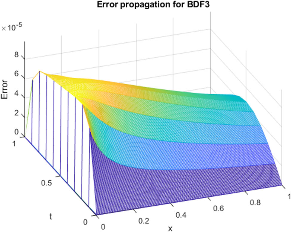
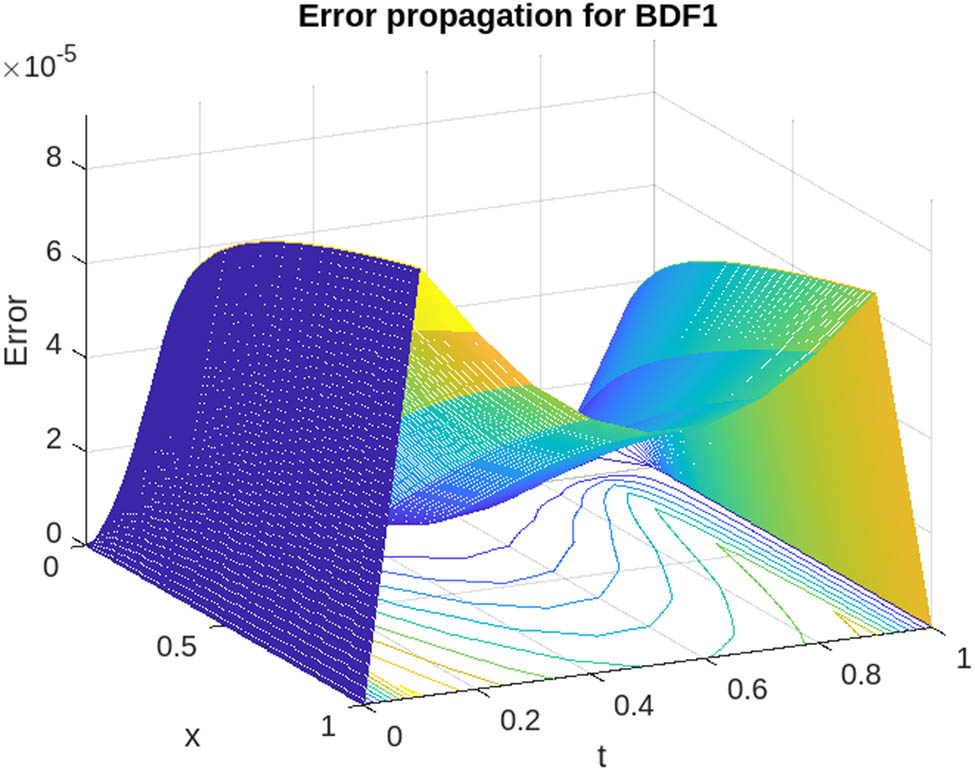
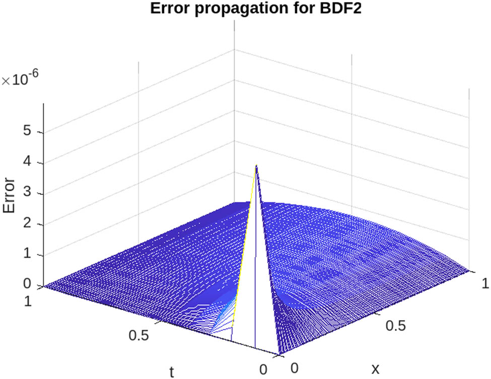
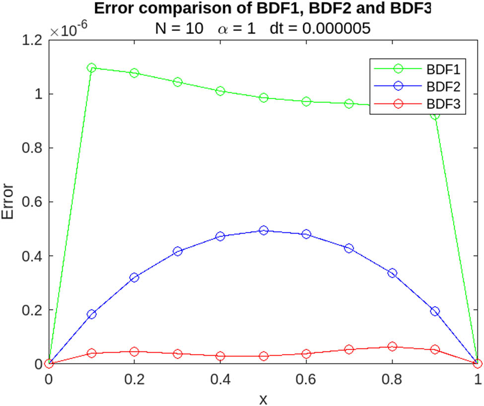
In this study, we compare numerical results and exact solutions derived from different BDFs. Tables 1 and 2 focus on the evaluation of three BDF methods at fixed time instances but varying spatial positions, providing insights into their spatial performance. In parallel, Tables 3 and 4 explore error comparisons under consistent time points but different spatial locations, offering valuable information about precision. Figures 1, 2, 3, 4, 5, 6 illustrate the computed solutions produced by BDF methods of first, second, and third orders, together with the exact solution, across a range of alpha values. In Figures 7 and 8, the absolute errors are depicted at the same time points but in different spatial locations. In a concurrent analysis, we expanded our comparison by using a time step of
Comparison of numerical and exact solutions (BDF1, BDF2, BDF3) for Example 1 at
|
|
BDF1 | BDF2 | BDF3 | Exact solution |
|---|---|---|---|---|
| 0.2 | 0.250420019 | 0.250420775 | 0.250421049 | 0.250421096 |
| 0.3 | 0.240310644 | 0.240311272 | 0.240311649 | 0.240311688 |
| 0.4 | 0.230417375 | 0.230417912 | 0.230418355 | 0.230418385 |
| 0.5 | 0.220747663 | 0.220748154 | 0.220748619 | 0.220748648 |
| 0.6 | 0.211308229 | 0.211308721 | 0.211309162 | 0.211309201 |
| 0.7 | 0.202105045 | 0.202105581 | 0.202105956 | 0.202106010 |
| 0.8 | 0.193143323 | 0.193143940 | 0.193144212 | 0.193144276 |
| 0.9 | 0.184427509 | 0.184428235 | 0.184428378 | 0.184428430 |
Comparison of numerical and exact solutions (BDF1, BDF2, BDF3) for Example 1 at
|
|
BDF1 | BDF2 | BDF3 | Exact solution |
|---|---|---|---|---|
| 0.1 | 0.3584088969 | 0.3584211896 | 0.3584221152 | 0.3584269144 |
| 0.2 | 0.3299634211 | 0.3299734888 | 0.3299752538 | 0.3299842051 |
| 0.3 | 0.3022946501 | 0.3023027800 | 0.3023052162 | 0.3023174246 |
| 0.4 | 0.2755792279 | 0.2755858557 | 0.2755887275 | 0.2756031473 |
| 0.5 | 0.2499758181 | 0.2499814841 | 0.2499845115 | 0.2500000000 |
| 0.6 | 0.2256212575 | 0.2256265533 | 0.2256294397 | 0.2256447723 |
| 0.7 | 0.2026276009 | 0.2026331139 | 0.2026355750 | 0.2026494300 |
| 0.8 | 0.1810801962 | 0.1810864553 | 0.1810882474 | 0.1810991715 |
| 0.9 | 0.1610368521 | 0.1610442798 | 0.1610452236 | 0.1610515941 |
Error comparison (BDF1, BDF2, BDF3) for Example 1 at
|
|
BDF1 | BDF2 | BDF3 |
|---|---|---|---|
| 0.1 |
|
|
|
| 0.2 |
|
|
|
| 0.3 |
|
|
|
| 0.4 |
|
|
|
| 0.5 |
|
|
|
| 0.6 |
|
|
|
| 0.7 |
|
|
|
| 0.8 |
|
|
|
| 0.9 |
|
|
|
Error comparison (BDF1, BDF2, BDF3) for Example 1 at
|
|
BDF1 | BDF2 | BDF3 |
|---|---|---|---|
| 0.1 |
|
|
|
| 0.2 |
|
|
|
| 0.3 |
|
|
|
| 0.4 |
|
|
|
| 0.5 |
|
|
|
| 0.6 |
|
|
|
| 0.7 |
|
|
|
| 0.8 |
|
|
|
| 0.9 |
|
|
|
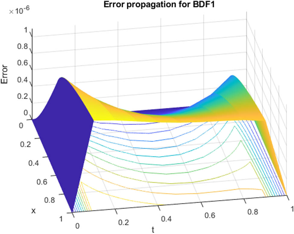
Error propagation of Example 1 at
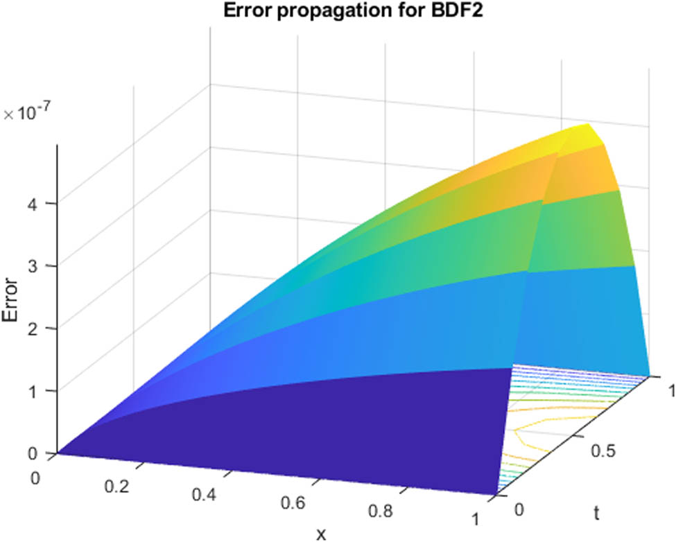
Error propagation of Example 1 at
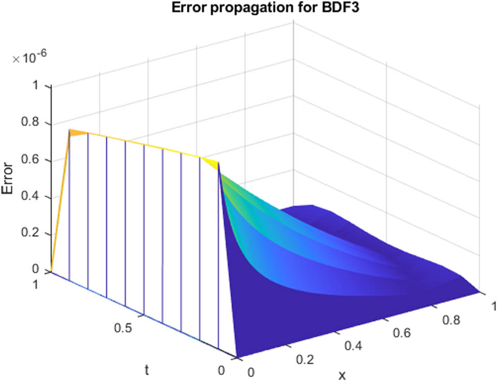
Error propagation of Example 1 at
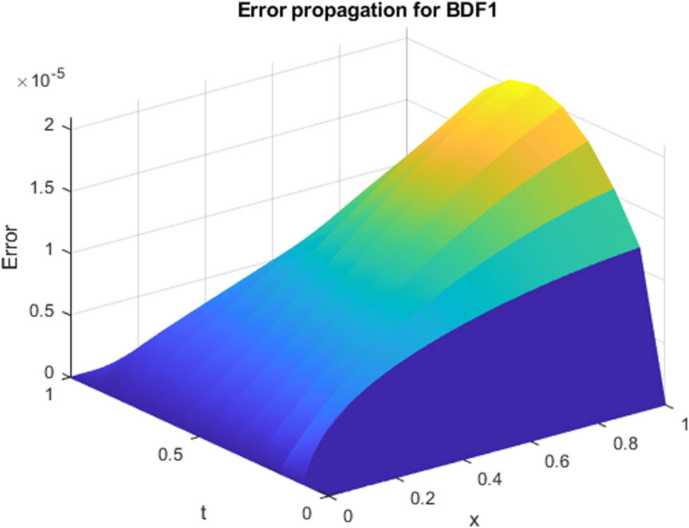
Error propagation of Example 1 at

Error propagation of Example 1 at

Error propagation of Example 1 at
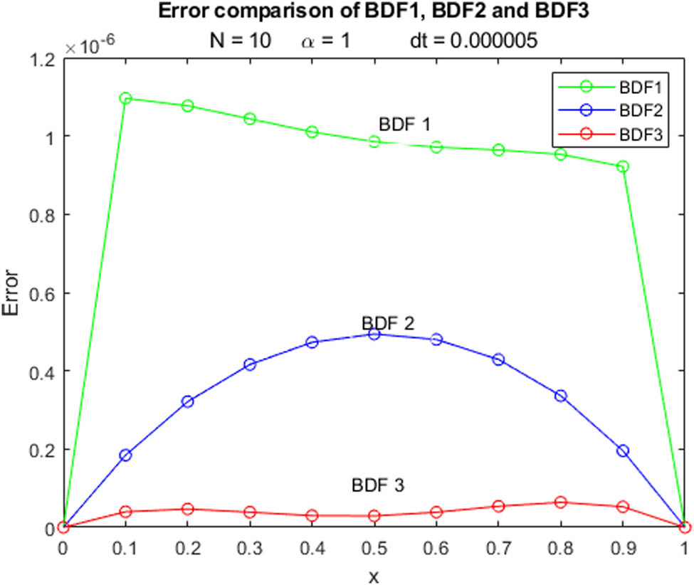
Error comparison of Example 1 at
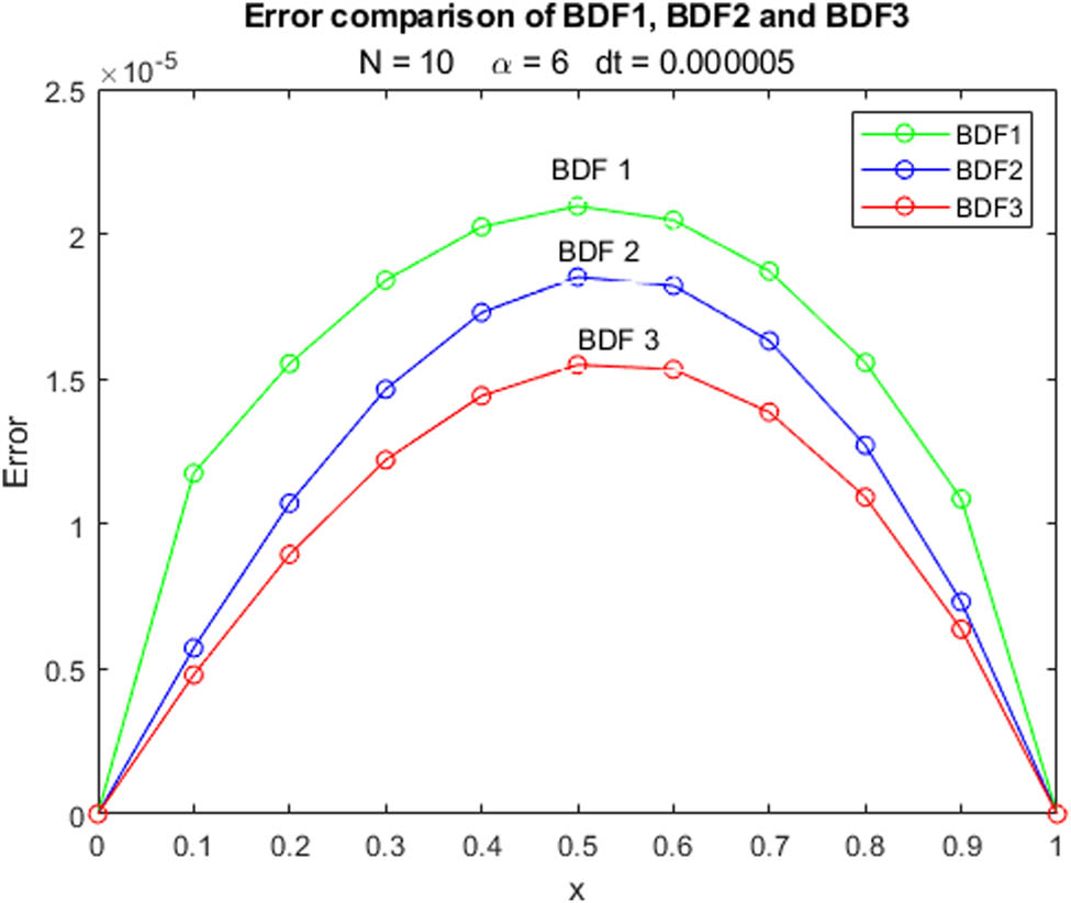
Error comparison of Example 1 at
Comparison of numerical and exact solutions (BDF1, BDF2, BDF3) for Example 1 at
| Computed solution | Exact solution | |||
|---|---|---|---|---|
|
|
BDF1 | BDF2 | BDF3 | |
| 0.1 | 0.260555346 | 0.260738174 | 0.260752490 | 0.260738428 |
| 0.2 | 0.250268689 | 0.250420646 | 0.250447850 | 0.250421096 |
| 0.3 | 0.240184531 | 0.240311103 | 0.240348491 | 0.240311688 |
| 0.4 | 0.230309036 | 0.230417726 | 0.230461597 | 0.230418385 |
| 0.5 | 0.220648412 | 0.220747972 | 0.220794013 | 0.220748648 |
| 0.6 | 0.211208986 | 0.211308559 | 0.211352270 | 0.211309201 |
| 0.7 | 0.201997201 | 0.202105453 | 0.202142581 | 0.202106010 |
| 0.8 | 0.193019543 | 0.193143852 | 0.193170799 | 0.193144276 |
| 0.9 | 0.184282411 | 0.184428190 | 0.184442349 | 0.184428430 |
Comparison of numerical and exact solutions (BDF1, BDF2, BDF3) for Example 1 at
| Computed solution | Exact solution | |||
|---|---|---|---|---|
|
|
BDF1 | BDF2 | BDF3 | |
| 0.1 | 0.357193283 | 0.358420734 | 0.358512716 | 0.358426914 |
| 0.2 | 0.328968781 | 0.329972662 | 0.330148039 | 0.329984205 |
| 0.3 | 0.301492288 | 0.302301712 | 0.302543759 | 0.302317425 |
| 0.4 | 0.274925758 | 0.275584698 | 0.275870007 | 0.275603147 |
| 0.5 | 0.249417565 | 0.249980376 | 0.250281128 | 0.250000000 |
| 0.6 | 0.225099525 | 0.225625602 | 0.225912319 | 0.225644772 |
| 0.7 | 0.202084201 | 0.202632381 | 0.202876840 | 0.202649430 |
| 0.8 | 0.180462762 | 0.181085967 | 0.181263959 | 0.181099172 |
| 0.9 | 0.160303577 | 0.161044038 | 0.161137779 | 0.161051594 |
Error comparison (BDF1, BDF2, BDF3) for Example 1 at
|
|
BDF1 | BDF2 | BDF3 |
|---|---|---|---|
| 0.1 | 0.000183082 |
|
|
| 0.2 | 0.000152407 |
|
|
| 0.3 | 0.000127158 |
|
|
| 0.4 | 0.000109349 |
|
|
| 0.5 | 0.000100236 |
|
|
| 0.6 | 0.000100215 |
|
|
| 0.7 | 0.000108809 |
|
|
| 0.8 | 0.000124734 |
|
|
| 0.9 | 0.000146020 |
|
|
Error comparison (BDF1, BDF2, BDF3) for Example 1 at
|
|
BDF1 | BDF2 | BDF3 |
|---|---|---|---|
| 0.1 | 0.001233632 |
|
|
| 0.2 | 0.001015424 |
|
0.000163834 |
| 0.3 | 0.000825137 |
|
0.000226335 |
| 0.4 | 0.000677389 |
|
0.000266860 |
| 0.5 | 0.000582435 |
|
0.000281128 |
| 0.6 | 0.000545247 |
|
0.000267547 |
| 0.7 | 0.000565229 |
|
0.000227410 |
| 0.8 | 0.000636410 |
|
0.000164788 |
| 0.9 | 0.000748017 |
|
|

Error propagation at

Error propagation at
Error propagation at

Error propagation at

Error propagation at

Error propagation at

Error comparison of Example 1 at

Error comparison of Example 1 at
We further examined the numerical solutions of BDF1, BDF2, and BDF3 in Tables 9, 10, and 11, comparing them with findings from previous publications [30,31] under the specific conditions of
Numerical and exact solutions for Example 1 are compared at different points of space at
|
|
|
DQM [31] | BDF1 | Exact solution |
|---|---|---|---|---|
| 0.5 | 0.25 | 0.81847 | 0.818313 | 0.818393 |
| 0.75 | 0.72592 | 0.725715 | 0.725824 | |
| 1.0 | 0.25 | 0.98293 | 0.982909 | 0.982919 |
| 0.75 | 0.97208 | 0.972055 | 0.972071 |
Numerical and exact solutions for Example 1 are compared at different points of space at
|
|
|
DQM [31] | BDF2 | Exact solution |
|---|---|---|---|---|
| 0.5 | 0.25 | 0.81847 | 0.818394 | 0.818393 |
| 0.75 | 0.72592 | 0.725826 | 0.725824 | |
| 1.0 | 0.25 | 0.98293 | 0.982918 | 0.982919 |
| 0.75 | 0.97208 | 0.972070 | 0.972071 |
Numerical and exact solutions for Example 1 are compared at different points of space at
|
|
|
DQM [31] | BDF3 | Exact solution |
|---|---|---|---|---|
| 0.5 | 0.25 | 0.81847 | 0.818395 | 0.818393 |
| 0.75 | 0.72592 | 0.725826 | 0.725824 | |
| 1.0 | 0.25 | 0.98293 | 0.982918 | 0.982919 |
| 0.75 | 0.97208 | 0.972070 | 0.972071 |
Assessing differences using the
|
|
|
|||
|---|---|---|---|---|
|
|
|
|
|
|
| BDF1 | 0.002677279 | 0.008466298 |
|
|
| BDF2 | 0.002677279 | 0.008466298 |
|
|
| BDF3 | 0.002677279 | 0.008466298 |
|
|
Assessing differences using the
|
|
|
|||
|---|---|---|---|---|
|
|
|
|
|
|
| BDF1 | 0.000131399 | 0.000183082 | 0.000796513 | 0.001233631 |
| BDF2 |
|
|
|
|
| BDF3 |
|
|
0.000198383 | 0.000281128 |
Example 2
Consider the following Fisher’s equation-2 in domain [0, 1] for
with initial condition
The exact solution is presented in [12,30] by
In Tables 15 and 16, we calculate the numerical solutions for Example 2, considering different time steps, specifically
Comparison of numerical and exact solutions (BDF1, BDF2, BDF3) for Example 2 at
| Computed solution | Exact solution | |||
|---|---|---|---|---|
|
|
BDF1 | BDF2 | BDF3 | |
| 0.1 | 0.260736413 | 0.2607382437 | 0.260738388 | 0.260738428 |
| 0.2 | 0.250419251 | 0.2504207746 | 0.250421049 | 0.250421096 |
| 0.3 | 0.240310001 | 0.2403112721 | 0.240311649 | 0.240311688 |
| 0.4 | 0.230416819 | 0.2304179122 | 0.230418355 | 0.230418385 |
| 0.5 | 0.220747153 | 0.2207481544 | 0.220748619 | 0.220748648 |
| 0.6 | 0.211307719 | 0.2113087208 | 0.211309162 | 0.211309201 |
| 0.7 | 0.202104493 | 0.2021055807 | 0.202105956 | 0.202106010 |
| 0.8 | 0.193142693 | 0.1931439398 | 0.193144212 | 0.193144276 |
| 0.9 | 0.184426775 | 0.1844282347 | 0.184428378 | 0.184428430 |
Error Comparison (BDF1, BDF2, BDF3) for Example 2 at
|
|
BDF1 | BDF2 | BDF3 |
|---|---|---|---|
| 0.1 |
|
|
|
| 0.2 |
|
|
|
| 0.3 |
|
|
|
| 0.4 |
|
|
|
| 0.5 |
|
|
|
| 0.6 |
|
|
|
| 0.7 |
|
|
|
| 0.8 |
|
|
|
| 0.9 |
|
|
|
Error Comparison (BDF1, BDF2, BDF3) for Example 2 at
|
|
BDF1 | BDF2 | BDF3 |
|---|---|---|---|
| 0.1 |
|
|
|
| 0.2 |
|
|
|
| 0.3 |
|
|
|
| 0.4 |
|
|
|
| 0.5 |
|
|
|
| 0.6 |
|
|
|
| 0.7 |
|
|
|
| 0.8 |
|
|
|
| 0.9 |
|
|
|
Error propagation at
Error propagation at

Error propagation at

Error propagation at

Error propagation at

Error propagation at
Error comparison at

Error comparison at
In Tables 19, 20, and 21, we evaluate the numerical solutions of BDF1, BDF2, and BDF3 compared to a few existing methods [30,31]. This assessment is performed under specific conditions, including
Comparing numerical results with exact solutions for Example 2 at various spatial positions, with a time step of
|
|
|
DQM [31] | BDF1 | Exact solution |
|---|---|---|---|---|
| 0.5 | 0.25 | 0.33412 | 0.334071 | 0.334094 |
| 0.75 | 0.27838 | 0.278332 | 0.278353 | |
| 1.0 | 0.25 | 0.45576 | 0.455714 | 0.455739 |
| 0.75 | 0.39544 | 0.395387 | 0.395411 |
Comparing numerical results with exact solutions for Example 2 at various spatial positions, with a time step of
|
|
|
DQM [31] | CFD6 [30] | BDF2 | Exact solution |
|---|---|---|---|---|---|
| 0.5 | 0.25 | 0.33412 | 0.334094 | 0.334094 | 0.334094 |
| 0.75 | 0.27838 | 0.278353 | 0.278353 | 0.278353 | |
| 1.0 | 0.25 | 0.45576 | 0.455739 | 0.455739 | 0.455739 |
| 0.75 | 0.39544 | 0.395411 | 0.395411 | 0.395411 |
Comparing numerical results with exact solutions for Example 2 at various spatial positions, with a time step of
|
|
|
DQM [31] | CFD6 [30] | BDF3 | Exact solution |
|---|---|---|---|---|---|
| 0.5 | 0.25 | 0.33412 | 0.334094 | 0.334094 | 0.334094 |
| 0.75 | 0.27838 | 0.278353 | 0.278353 | 0.278353 | |
| 1.0 | 0.25 | 0.45576 | 0.455739 | 0.455739 | 0.455739 |
| 0.75 | 0.39544 | 0.395411 | 0.395411 | 0.395411 |
Comparing numerical and exact solutions for Example 2 at various spatial points with
| BDF1 | BDF2 | BDF3 | |||||||
|---|---|---|---|---|---|---|---|---|---|
|
|
|
|
ROC |
|
|
ROC |
|
|
ROC |
| 10 |
|
|
|
|
|
||||
| 15 |
|
|
|
|
|
|
|
|
|
| 20 |
|
|
|
|
|
|
|
|
|
10 Conclusion
To transform the nonlinear Fisher equation into a set of first-order ODEs, we employ a semi-discretization method along the variable “
Acknowledgements
The authors are very thankful to the reviewers for their valuable comments and suggestions, which improved the quality of this study.
-
Funding information: The authors state that there is no funding involved.
-
Author contributions: All authors have accepted responsibility for the entire content of this manuscript and approved its submission.
-
Conflict of interest: The authors declare that there is no conflict of interest.
-
Data availability statement: All data, generated or used during the study, are available within the article.
References
[1] Fisher RA. The wave of advance of advantageous genes. Ann Eugenics. 1937;7(4):355–69. 10.1111/j.1469-1809.1937.tb02153.xSuche in Google Scholar
[2] Kudryashov NA, Zakharchenko AS. A note on solutions of the generalized Fisher equation. Appl Math Lett. 2014;32:53–6. 10.1016/j.aml.2014.02.009Suche in Google Scholar
[3] Ablowitz MJ, Zeppetella A. Explicit solutions of Fisher’s equation for a special wave speed. Bulletin Math Biol. 1979;41(6):835–40. 10.1016/S0092-8240(79)80020-8Suche in Google Scholar
[4] Korpusov M, Ovchinnikov A, Sveshnikov A. On blow up of generalized Kolmogorov-Petrovskii-Piskunov equation. Nonlinear Anal Theory Methods Appl. 2009;71(11):5724–32. 10.1016/j.na.2009.05.002Suche in Google Scholar
[5] Kudryashov NA. Exact solitary waves of the Fisher equation. Phys Lett A. 2005;342(1–2):99–106. 10.1016/j.physleta.2005.05.025Suche in Google Scholar
[6] Vitanov NK, Jordanov IP, Dimitrova ZI. On nonlinear population waves. Appl Math Comput. 2009;215(8):2950–64. 10.1016/j.amc.2009.09.041Suche in Google Scholar
[7] Frank-Kamenetskii DA. Diffusion and heat transfer in chemical kinetics. Princeton: Princeton University Press. vol. 2171; 2015.Suche in Google Scholar
[8] Ammerman AJ, Cavalli-Sforza LL. Measuring the rate of spread of early farming in Europe. Man. Royal Anthropological Institute of Great Britain and Ireland. vol. 6; 1971. p. 674–88.10.2307/2799190Suche in Google Scholar
[9] Bramson MD. Maximal displacement of branching Brownian motion. Commun Pure Appl Math. 1978;31(5):531–81. 10.1002/cpa.3160310502Suche in Google Scholar
[10] Canosa J. Diffusion in nonlinear multiplicative media. J Math Phys. 1969;10(10):1862–8. 10.1063/1.1664771Suche in Google Scholar
[11] Chandraker V, Awasthi A, Jayaraj S. A numerical treatment of Fisher equation. Proc Eng. 2015;127:1256–62. 10.1016/j.proeng.2015.11.481Suche in Google Scholar
[12] Wang X. Exact and explicit solitary wave solutions for the generalised Fisher equation. Phys Lett A. 1988;131(4–5):277–9. 10.1016/0375-9601(88)90027-8Suche in Google Scholar
[13] Branco J, Ferreira J, De Oliveira P. Numerical methods for the generalized Fisher-Kolmogorov-Petrovskii-Piskunov equation. Appl Numer Math. 2007;57(1):89–102. 10.1016/j.apnum.2006.01.002Suche in Google Scholar
[14] Macías-Díaz JE, Medina-Ramírez I, Puri A. Numerical treatment of the spherically symmetric solutions of a generalized Fisher-Kolmogorov-Petrovsky-Piscounov equation. J Comput Appl Math. 2009;231(2):851–68. 10.1016/j.cam.2009.05.008Suche in Google Scholar
[15] Agbavon KM, Appadu AR, Inan B, Tenkam HM. Convergence analysis and approximate optimal temporal step sizes for some finite difference methods discretising Fisher’s equation. Front Appl Math Stat. 2022;8:921170. 10.3389/fams.2022.921170Suche in Google Scholar
[16] Abd-Elhameed W, Ali A, Youssri YH. Newfangled linearization formula of certain Nonsymmetric Jacobi polynomials: Numerical treatment of nonlinear Fisheras equation. J Funct Spaces. 2023;2023(1):6833404. 10.1155/2023/6833404Suche in Google Scholar
[17] Hanaç Duruk E, Koksal ME, Jiwari R. Analyzing similarity solution of modified fisher equation. J Math. 2022;2022:6806906. 10.1155/2022/6806906Suche in Google Scholar
[18] Hamrouni A, Choucha A, Alharbi A, Idris SA. Global existence of solution for the Fisher equation via Faedo-Galerkin’s method. J Math. 2021;2021:1–7. 10.1155/2021/3304917Suche in Google Scholar
[19] Fares MM, Abdelsalam UM, Allehiany FM. Travelling wave solutions for Fisher’s equation using the extended homogeneous balance method: travelling wavesolutions for Fisher’s equation. Sultan Qaboos Univ J Sci. 2021;26(1):22–30. 10.53539/squjs.vol26iss1pp22-30Suche in Google Scholar
[20] Rosa M, Chulián S, Gandarias M, Traciná R. Application of Lie point symmetries to the resolution of an interface problem in a generalized Fisher equation. Phys D: Nonlinear Phenomena. 2020;405:132411. 10.1016/j.physd.2020.132411Suche in Google Scholar
[21] Ahmad S, Ullah A, Ullah A, Akgül A, Abdeljawad T. Computational analysis of fuzzy fractional order non-dimensional Fisher equation. Phys Scr. 2021;96(8):084004. 10.1088/1402-4896/abfaceSuche in Google Scholar
[22] Schiesser WE. The numerical method of lines: integration of partial differential equations. Elsevier; 2012Suche in Google Scholar
[23] Ilati M, Dehghan M. Direct local boundary integral equation method for numerical solution of extended Fisher-Kolmogorov equation. Eng Comput. 2018;34:203–13. 10.1007/s00366-017-0530-1Suche in Google Scholar
[24] Cheniguel A. Numerical method for the heat equation with Dirichlet and Neumann conditions. In: Proceedings of the International MultiConference of Engineers and Computer Scientists. vol. 1; 2014. p. 12–4. Suche in Google Scholar
[25] Ersoy O, Dag I. The numerical approach to the Fisher’s equation via trigonometriccubic B-spline collocation method. 2016. arXiv: http://arXiv.org/abs/arXiv:160406864. Suche in Google Scholar
[26] Oymak O, Selçuk N. Method-of-lines solution of time-dependenttwo-dimensional Navier-Stokes equations. Int J Numer Methods Fluids. 1996;23(5):455–66. 10.1002/(SICI)1097-0363(19960915)23:5<455::AID-FLD435>3.0.CO;2-JSuche in Google Scholar
[27] Atkinson K, Han W, Stewart DE. Numerical solution of ordinary differential equations. New Jersey: John Wiley and Sons; vol. 81; 2009.10.1002/9781118164495Suche in Google Scholar
[28] Aswin V, Awasthi A, Anu C. A comparative study of numerical schemes for convection-diffusion equation. Proc Eng. 2015;127:621–7. 10.1016/j.proeng.2015.11.353Suche in Google Scholar
[29] Wazwaz AM, Gorguis A. An analytic study of Fisher’s equation by using Adomian decomposition method. Appl Math Comput. 2004;154(3):609–20. 10.1016/S0096-3003(03)00738-0Suche in Google Scholar
[30] Bastani M, Salkuyeh DK. A highly accurate method to solve Fisher’s equation. Pramana. 2012;78:335–46. 10.1007/s12043-011-0243-8Suche in Google Scholar
[31] Mittal R, Jiwari R. Numerical study of Fisher’s equation by using differential quadrature method. Int J Inf Syst Sci. 2009;5(1):143–60. Suche in Google Scholar
© 2024 the author(s), published by De Gruyter
This work is licensed under the Creative Commons Attribution 4.0 International License.
Artikel in diesem Heft
- Editorial
- Focus on NLENG 2023 Volume 12 Issue 1
- Research Articles
- Seismic vulnerability signal analysis of low tower cable-stayed bridges method based on convolutional attention network
- Robust passivity-based nonlinear controller design for bilateral teleoperation system under variable time delay and variable load disturbance
- A physically consistent AI-based SPH emulator for computational fluid dynamics
- Asymmetrical novel hyperchaotic system with two exponential functions and an application to image encryption
- A novel framework for effective structural vulnerability assessment of tubular structures using machine learning algorithms (GA and ANN) for hybrid simulations
- Flow and irreversible mechanism of pure and hybridized non-Newtonian nanofluids through elastic surfaces with melting effects
- Stability analysis of the corruption dynamics under fractional-order interventions
- Solutions of certain initial-boundary value problems via a new extended Laplace transform
- Numerical solution of two-dimensional fractional differential equations using Laplace transform with residual power series method
- Fractional-order lead networks to avoid limit cycle in control loops with dead zone and plant servo system
- Modeling anomalous transport in fractal porous media: A study of fractional diffusion PDEs using numerical method
- Analysis of nonlinear dynamics of RC slabs under blast loads: A hybrid machine learning approach
- On theoretical and numerical analysis of fractal--fractional non-linear hybrid differential equations
- Traveling wave solutions, numerical solutions, and stability analysis of the (2+1) conformal time-fractional generalized q-deformed sinh-Gordon equation
- Influence of damage on large displacement buckling analysis of beams
- Approximate numerical procedures for the Navier–Stokes system through the generalized method of lines
- Mathematical analysis of a combustible viscoelastic material in a cylindrical channel taking into account induced electric field: A spectral approach
- A new operational matrix method to solve nonlinear fractional differential equations
- New solutions for the generalized q-deformed wave equation with q-translation symmetry
- Optimize the corrosion behaviour and mechanical properties of AISI 316 stainless steel under heat treatment and previous cold working
- Soliton dynamics of the KdV–mKdV equation using three distinct exact methods in nonlinear phenomena
- Investigation of the lubrication performance of a marine diesel engine crankshaft using a thermo-electrohydrodynamic model
- Modeling credit risk with mixed fractional Brownian motion: An application to barrier options
- Method of feature extraction of abnormal communication signal in network based on nonlinear technology
- An innovative binocular vision-based method for displacement measurement in membrane structures
- An analysis of exponential kernel fractional difference operator for delta positivity
- Novel analytic solutions of strain wave model in micro-structured solids
- Conditions for the existence of soliton solutions: An analysis of coefficients in the generalized Wu–Zhang system and generalized Sawada–Kotera model
- Scale-3 Haar wavelet-based method of fractal-fractional differential equations with power law kernel and exponential decay kernel
- Non-linear influences of track dynamic irregularities on vertical levelling loss of heavy-haul railway track geometry under cyclic loadings
- Fast analysis approach for instability problems of thin shells utilizing ANNs and a Bayesian regularization back-propagation algorithm
- Validity and error analysis of calculating matrix exponential function and vector product
- Optimizing execution time and cost while scheduling scientific workflow in edge data center with fault tolerance awareness
- Estimating the dynamics of the drinking epidemic model with control interventions: A sensitivity analysis
- Online and offline physical education quality assessment based on mobile edge computing
- Discovering optical solutions to a nonlinear Schrödinger equation and its bifurcation and chaos analysis
- New convolved Fibonacci collocation procedure for the Fitzhugh–Nagumo non-linear equation
- Study of weakly nonlinear double-diffusive magneto-convection with throughflow under concentration modulation
- Variable sampling time discrete sliding mode control for a flapping wing micro air vehicle using flapping frequency as the control input
- Error analysis of arbitrarily high-order stepping schemes for fractional integro-differential equations with weakly singular kernels
- Solitary and periodic pattern solutions for time-fractional generalized nonlinear Schrödinger equation
- An unconditionally stable numerical scheme for solving nonlinear Fisher equation
- Effect of modulated boundary on heat and mass transport of Walter-B viscoelastic fluid saturated in porous medium
- Analysis of heat mass transfer in a squeezed Carreau nanofluid flow due to a sensor surface with variable thermal conductivity
- Navigating waves: Advancing ocean dynamics through the nonlinear Schrödinger equation
- Experimental and numerical investigations into torsional-flexural behaviours of railway composite sleepers and bearers
- Novel dynamics of the fractional KFG equation through the unified and unified solver schemes with stability and multistability analysis
- Analysis of the magnetohydrodynamic effects on non-Newtonian fluid flow in an inclined non-uniform channel under long-wavelength, low-Reynolds number conditions
- Convergence analysis of non-matching finite elements for a linear monotone additive Schwarz scheme for semi-linear elliptic problems
- Global well-posedness and exponential decay estimates for semilinear Newell–Whitehead–Segel equation
- Petrov-Galerkin method for small deflections in fourth-order beam equations in civil engineering
- Solution of third-order nonlinear integro-differential equations with parallel computing for intelligent IoT and wireless networks using the Haar wavelet method
- Mathematical modeling and computational analysis of hepatitis B virus transmission using the higher-order Galerkin scheme
- Mathematical model based on nonlinear differential equations and its control algorithm
- Bifurcation and chaos: Unraveling soliton solutions in a couple fractional-order nonlinear evolution equation
- Space–time variable-order carbon nanotube model using modified Atangana–Baleanu–Caputo derivative
- Minimal universal laser network model: Synchronization, extreme events, and multistability
- Valuation of forward start option with mean reverting stock model for uncertain markets
- Geometric nonlinear analysis based on the generalized displacement control method and orthogonal iteration
- Fuzzy neural network with backpropagation for fuzzy quadratic programming problems and portfolio optimization problems
- B-spline curve theory: An overview and applications in real life
- Nonlinearity modeling for online estimation of industrial cooling fan speed subject to model uncertainties and state-dependent measurement noise
- Quantitative analysis and modeling of ride sharing behavior based on internet of vehicles
- Review Article
- Bond performance of recycled coarse aggregate concrete with rebar under freeze–thaw environment: A review
- Retraction
- Retraction of “Convolutional neural network for UAV image processing and navigation in tree plantations based on deep learning”
- Special Issue: Dynamic Engineering and Control Methods for the Nonlinear Systems - Part II
- Improved nonlinear model predictive control with inequality constraints using particle filtering for nonlinear and highly coupled dynamical systems
- Anti-control of Hopf bifurcation for a chaotic system
- Special Issue: Decision and Control in Nonlinear Systems - Part I
- Addressing target loss and actuator saturation in visual servoing of multirotors: A nonrecursive augmented dynamics control approach
- Collaborative control of multi-manipulator systems in intelligent manufacturing based on event-triggered and adaptive strategy
- Greenhouse monitoring system integrating NB-IOT technology and a cloud service framework
- Special Issue: Unleashing the Power of AI and ML in Dynamical System Research
- Computational analysis of the Covid-19 model using the continuous Galerkin–Petrov scheme
- Special Issue: Nonlinear Analysis and Design of Communication Networks for IoT Applications - Part I
- Research on the role of multi-sensor system information fusion in improving hardware control accuracy of intelligent system
- Advanced integration of IoT and AI algorithms for comprehensive smart meter data analysis in smart grids