Research on the role of multi-sensor system information fusion in improving hardware control accuracy of intelligent system

Xin Li; Yuesong Li

doi:10.1515/nleng-2024-0035

Enjoy 40% off

academic books on De Gruyter Brill *

Article Open Access

Research on the role of multi-sensor system information fusion in improving hardware control accuracy of intelligent system

Xin Li and Yuesong Li

Published/Copyright: October 25, 2024

Published by

Become an author with De Gruyter Brill

Submit Manuscript Author Information

From the journal Nonlinear Engineering Volume 13 Issue 1

Abstract

Multi-sensor management and control technology generally constructs a reasonable objective function to solve the optimal control command set to control a limited number of sensors to obtain higher quality measurement information, thus obtaining better target tracking performance. In the process of multi-sensor information fusion, there is not only the problem of information redundancy but also obvious time delay. A sensor fusion algorithm combined with global optimization algorithm is innovatively proposed. According to the key frames saved in the previous steps, feature points in local maps, sensor information, and loop information, a global optimization algorithm based on graph optimization model is constructed to optimize the position and pose of intelligent hardware system and the position of spatial feature points. Moreover, this work studies and experiments on multi-sensor fusion simultaneous localization and mapping (SLAM) comprehensively and systematically, and the experimental results show that the algorithm proposed in this work is superior to common open-source SLAM algorithm in positioning accuracy and mapping effect under special circumstances. Therefore, the method proposed in this work can be applied to intelligent driving of vehicles, vision-assisted movement of robots and intelligent control of unmanned aerial vehicles, thus effectively improving the hardware control accuracy of intelligent systems.

Keywords: multi-sensor system; information fusion; intelligent system; SALM

1 Introduction

With the rapid development of electronic technology and information technology, the information obtained by a single sensor can no longer meet people’s requirements for data. Multi-sensor information fusion is a new subject, which can analyze and process multiple sensors or data according to some optimal fusion rules by computer technology, so as to obtain more accurate system state. Compared with a single sensor which can only measure a single aspect or a certain range, multi-sensor information fusion can obtain more comprehensive information of the target, get more accurate estimation accuracy, reduce the uncertain factors of the target, and improve the stability, flexibility, and credibility of the system.

In recent years, due to the large-scale production of intelligent sensors, wireless sensor networks (WSNs) with advantages such as low cost, easy installation and maintenance, and lightweight have developed rapidly. As an emerging technology, WSNs are widely used in various practical fields due to their multifunctional characteristics and collaborative behavior

In the study of control systems, if the time delay is relatively small, it will not have a significant impact on the stability and accuracy of the system. However, when modeling and estimating control systems, time delay is often ignored to simplify model calculations. But, in general, the phenomenon of time delay cannot be avoided or ignored, and classical Kalman filtering can only be applied to standard models and is no longer applicable to time delay models. Therefore, the study of time delay models has important theoretical value and practical application significance.

Through the above analysis, we can see that in the process of multi-sensor information fusion, there are not only information redundancy problems but also obvious time delay problems. To improve the intelligent control precision of multi-sensor system, the timeliness of information fusion and propagation is very important. Therefore, improving the information fusion effect of multi-sensor system is an inevitable way to improve the hardware control accuracy of intelligent system. The aim of this work is to improve the hardware control accuracy of intelligent system by improving the information fusion effect of multi-sensor system, reduce the redundancy of information fusion through algorithm improvement, and further reduce the information delay. Moreover, this study innovatively proposes a sensor fusion algorithm combined with global optimization algorithm, and constructs a global optimization algorithm based on graph optimization model according to the key frames saved in the previous steps, feature points in local maps, sensor information and loop information, and optimizes the position and pose of intelligent hardware system. In addition, this work studies and experiments on multi-sensor fusion simultaneous localization and mapping (SLAM) comprehensively and systematically, and the experimental results show that the algorithm proposed in this work is superior to common open-source SLAM algorithm in positioning accuracy and map building effect.

In this study, a sensor fusion algorithm combined with global optimization algorithm is innovatively proposed. According to the key frames saved in the previous steps, feature points in local maps, sensor information, and loop information, a global optimization algorithm based on graph optimization model is constructed to optimize the position and pose of intelligent hardware system and the position of spatial feature points. Moreover, this work studies and experiments on multi-sensor fusion SLAM comprehensively and systematically, and the experimental results show that the algorithm proposed in this study is superior to common open-source SLAM algorithm in positioning accuracy and mapping effect under special circumstances.

2 Related work

Multi target tracking is the process of predicting, updating, and continuously estimating the states of multiple targets through filtering algorithms. However, tracking scenarios are often complex and variable, and targets may appear or disappear anytime and anywhere. The detection of sensors may have missed detections, false alarms, and interference from clutter, resulting in a highly challenging problem of state estimation for multiple targets [1]. Traditional multi-target tracking usually involves track management steps such as track initiation, track termination, and track deletion. The corresponding relationship between the target and the measurement is established through data association, and then filtering and updating are performed between each association pair. The multi-target tracking algorithm based on random sets models the multi-target density as a set density, which can better describe unknown and time-varying multi-target states. The tracking process avoids explicit data correlation and does not require trajectory management. Moreover, the overall tracking filtering framework is more concise and convenient for debugging. Therefore, filtering algorithms based on random set theory have been widely studied and applied in the field of multi-target tracking [2].

Due to the fact that multi-objective Bayesian filters involve the calculation of set integrals, in order to solve the problem of difficulty, Kashinath et al. [3] proposed a highly representative Probability hypothesis density (PHD) filter. The PHD filter transfers the first-order moment approximation of the posterior density of multiple targets during the iteration process, transferring the multi-target tracking problem to the single target state space for solution, greatly reducing computational complexity. However, the iterative calculation of PHD filtering involves the integration problem of multi-dimensional vectors, and there is usually no closed form analytical solution. To address this issue, Liu et al. [4] proposed the Sequential Monte Carlo method and Gaussian mixture (GM) method to achieve closed form recursion of PHD. The derivation of PHD filters is based on the assumption that the target cardinality distribution follows a Poisson distribution. Since the mean of the Poisson distribution is equal to the variance, if there are many targets, the cardinality estimation of the targets will become extremely unstable due to the large variance, which is prone to significant deviation and fluctuation [5]. Zou et al. [6] proposed the Cardinalized probability hypothesis density (CPHD) filters. The CPHD filter iteratively estimates the first-order moment of the posterior density of multiple targets and the cardinality distribution of multiple targets, thus obtaining a more accurate estimate of the number of targets. However, the computational complexity of this filter is higher than that of the PHD filter.

In a distributed multi-sensor network, each sensor node independently observes target motion, performs filtering processing locally to generate local multi-target tracking results, and then sends them to the fusion center for data association and fusion, forming a global multi-target state estimation. Distributed data fusion is essentially the average calculation of posterior information from various sensor nodes, which is usually divided into two methods: Weighted arithmetic average (WAA) and Weighted geometric average (WGA) [7]. Among them, WAA fusion is based on linear combination [8] and can be explained as minimizing the weighted sum of Cauchy–Schwarz (CS) divergence between fusion density and local density. WGA fusion is based on exponential mixing [9], which can be explained as minimizing the weighted sum of Kullback–Leibler (KL) divergence between fusion density and local density.

The above fusion algorithms are proposed when each sensor’s field of view covers the entire monitoring area. However, in practical applications, the field of view of sensors is often limited, and a single sensor may not be able to observe the entire monitoring area. Therefore, local multi-target tracking results are prone to missed detections.

Multi-sensor control generally includes three important modules: multi-target tracking filtering process, multi-sensor information fusion process, and multi-sensor decision optimization process [10]. Among them, the decision optimization process is the core of solving multi-sensor control problems, usually relying on the construction and optimization of the objective function. According to the different types of objective functions, multi-sensor control algorithms can be divided into two categories: task driven and information driven. In task driven control methods, the objective function is usually expressed as a cost function, which directly depends on the evaluation indicators of quantitative tracking performance, such as the state variance and cardinality variance of multi-objective posterior estimation [11]. In information driven control methods, the objective function is usually represented as a reward function, which often depends on the amount of information in the multi-objective posterior distribution or the information gain of the posterior density relative to the prior density, which is usually measured by information entropy based on information theory.

Recently, on the basis of multi-sensor control algorithms for multi-target tracking, considering the limited field of view of sensors and meeting the requirements of search and tracking, multi-sensor control algorithms have gradually developed [12]. Due to limited field of view, each sensor node can only observe a small area and needs to collaborate with other nodes in the sensor network to maximize the search and tracking performance of the entire sensor network. However, achieving multi-sensor control with multiple competitive objective functions is a challenging problem, which requires each sensor to make a trade-off between searching for new targets and tracking discovered targets. The complex interaction between sensors can lead to combinatorial optimization problems. In addition, in actual tracking, missed detections and false alarms may also occur, as well as targets may enter and leave the sensor field of view at any time. This makes it even more difficult to address the problem of multi-sensor control for simultaneous search and tracking [13]. Guo et al. [14] solved the problem of sensor search and tracking by establishing an uncertainty threshold based on information theory to trigger a pre-planned search pattern. Tran et al. [15], using grid occupancy to represent the presence of undetected targets, proposed a search tracking joint objective function with mutual information as the information gain, and proved that the objective function is a single tone submodular set function, which can be approximated by a greedy algorithm to obtain the optimal solution (1-1/e). Lv et al. [16] established a multi-agent path planning algorithm based on PHD filters, which maximizes the number of expected targets detected by sensors for sensor control, so as to detect static targets to the maximum extent possible. Wu et al. [17] combined a PHD filter with a control method based on the Voronoi diagram, using the output of a distributed PHD filter to weigh the relative importance of the regions within the Voronoi unit, enabling a group of mobile sensors to simultaneously search and track an unknown number of targets. Zhang et al. [18] proposed a search and tracking solution based on poisson multi-Bernoulli mixture filters, which utilizes a task driven joint objective function for single sensor control. Lin et al. [19] proposed an improved scheme for the new target model, which allows for sharp edges or abrupt changes in the intensity of undetected targets around the sensor’s field of view without the use of a large number of GM components, reducing computational complexity compared to traditional methods. Du et al. [20] proposed a new unit multi-Bernoulli distribution to characterize multi-objective random finite set for multi-objective information gain functions that satisfy unit additivity constraints. The desired set function has a tractable high-order approximation, and without relying on the predicted ideal set of measurements, it derives a reward function expression with KL divergence as a measure of information gain, and solves the optimal control action by maximizing the reward function, thereby guiding the sensor to perform search and tracking.

3 Multi-sensor fusion algorithm model

3.1 Sensor fusion

Considering the large number of sensors used in intelligent hardware system pose estimation, especially the visual camera’s ability to obtain a large amount of environmental information, direct graph optimization inevitably leads to an increase in computational complexity. Therefore, based on the current pose estimation information, key frames are selected, local maps are constructed, and all original sensor information is saved for subsequent optimization. Second, considering that intelligent hardware systems may move for a long time in the same environment, there is a high possibility of loops in the motion path, and the images obtained by visual cameras contain a large number of environmental features. Therefore, the study introduces a loop detection mechanism based on image information to search for loops. Based on the keyframes saved in the previous steps, feature points in the local map, sensor information, and loop information, a global optimization algorithm (the principle of global optimization algorithm is to make real-time judgments on the environment through the fusion of information from multiple environmental information sensors, generate a global map, and make comprehensive judgments based on the collected information to optimize the shortcomings reasonably) based on graph optimization model is constructed to optimize the pose and spatial feature point positions of the intelligent hardware system, reducing the pose estimation error and spatial feature point position error of the intelligent hardware system. Finally, a two-dimensional map is generated by combining LiDAR data, and a multi-source global map is formed by combining spatial feature points.

Figure 1 shows the algorithm framework constructed in this work, which includes five parts: input, local map building, loop detection, global optimization, and output.

Figure 1

Analysis of multi-sensor fusion algorithm steps.

As shown in Figure 1, the construction of local maps includes two processes: keyframe selection and feature point sparsity, both aimed at simplifying data and reducing algorithm computation. Among them, keyframes are selected based on certain selection criteria to leave some data frames, while the remaining data frames are directly deleted. On the other hand, the feature point position data in the remaining data frames can be directly combined with the LiDAR data to construct a local map. However, the same feature point in the local map may be observed by cameras in multiple keyframes, resulting in a certain degree of redundancy. Directly using it for optimization will consume a lot of computing power. Moreover, in some local locations on the map, there are too many feature points, which have little impact on the quality of local map construction. Removing redundant feature points can also optimize the storage and transmission process of long-term and large-scale mapping. Therefore, it is necessary to further sparsify the feature points.

Taking the corridor space as an example, the motion of intelligent terminal devices in the corridor space can be regarded as the movement of a bounded area. By combining keyframes, feature points in local maps, sensor information, and loop information, a global optimization algorithm based on a graph optimization model is constructed to optimize their spatial position points, minimize position errors, and form a multi-source global map by combining spatial feature points.

Considering that intelligent hardware systems may move for a long time in the same environment, there may be a large amount of backhaul motion during the operation of the intelligent hardware system. Due to the influence of accumulated errors, there may be significant differences in the pose estimation of the intelligent hardware system at the same position. Loop detection can detect whether the intelligent hardware system has passed through the same or similar position previously. If a loop is detected between the current frame and the previous frame, a loop edge can be added to the subsequent graph optimization model. During global optimization, the solver will consider the loop constraint to reduce cumulative errors. Compared to visual information, the two-dimensional LiDAR point cloud data used in this study is relatively sparse, and the obtained environmental features are limited. Therefore, based on image information for loop detection, the specific implementation scheme is the word bag method. After the above data processing, a sparse feature point map and loop information were obtained. Based on this, a multi-sensor fusion optimization algorithm based on a graph optimization model was constructed by combining the input sensor information to further optimize the pose of the intelligent hardware system in key frames and the position of spatial feature points. The main steps include constructing a graph, constructing an objective function, and solving the objective function. Finally, the precise pose and spatial feature points of the intelligent hardware system were obtained through global optimization, and combined with the raw data of the LiDAR, a global map can be constructed and output.

3.2 Global optimization

The selection of key frames is essentially a data reduction process, which can reduce the amount of subsequent calculation and still ensure the restoration of the map. The criteria for selecting key frames in this section are as follows: (1) The time interval between the current frame and the previous key frame is greater than the preset threshold. (2) The distance and attitude difference between the key frame of the current frame and the previous frame is greater than the preset threshold.

When the key frame is selected, the feature point map can be constructed by combining the feature points after feature triangulation. As shown in Figure 2, the feature point map shown in the figure is another set of data of OpenLORIS-Scene dataset coffee shop scene, and the feature points in the figure also include the motion track of intelligent hardware system.

Figure 2

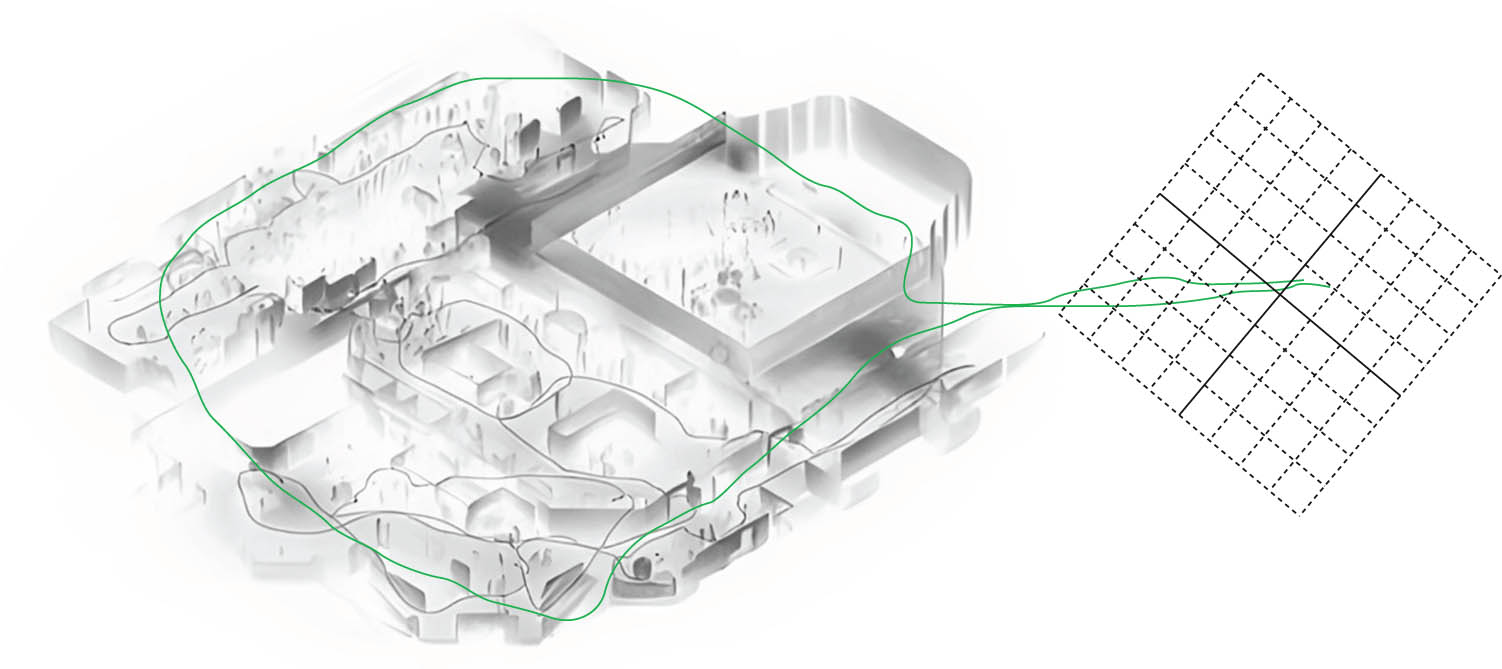
Feature point map.

The feature point sparse method based on quadratic programming is used to remove redundant feature points in the map. The optimization model is as follows:

(1) x ∗ = arg min 1 2 x T Q x + q T x + λ 1 T s .t A x ≥ b 1 ∑ t = 1 N x i = n x ∈ { 0 , 1 } N ς ∈ { { 0 } ∪ Z + } M ,

where x is a binary vector, and the ith element in the vector indicates whether the ith feature point is retained in the map. If the feature point is preserved, it is 1, otherwise it is 0. A is a matrix of M × N , M is the number of key frames, and N is the number of feature points. q is a first-order weight vector, and b represents the minimum number of feature points to be retained in each key frame, and q and b need to be constantly adjusted in the iterative solution process. Q is the quadratic weight matrix, in which the element Q i j is set as follows:

(2) Q i j = ∑ k = 1 m 0 , d min − ∥ p k , i − p k , j ∥ d min m ,

where p k , i and p k , j represent the positions of i th and j th feature points in k th key frames, respectively, the norm between them represents the distance between two points, d min represents the threshold value, and m represents the number of key frames. Binomial weight matrix Q will punish the feature points projected to nearby images when observing key frames.

According to the quadratic programming model given in formula (1), the feature points in the map can be simplified, and the remaining feature points become sparse feature point maps. Figure 3 is the result of sparse feature point maps shown in Figure 2.

Figure 3

Map of sparse feature points.

Using the Bag-of-Words model in visual processing to detect the loop, the main process is as follows: First, the dictionary is constructed. Dictionary is composed of words in the image. Words come from feature descriptors, which is a combination of features, and dictionary construction is a clustering problem of descriptors, and the construction process of dictionary can be carried out offline. K-means clustering algorithm is used to construct a dictionary according to the feature points and descriptors in the image, and K-tree structure is used to save the dictionary to ensure the efficiency of word search. Then, create an image word bag. For any feature in the image, we can find the corresponding words in the dictionary layer by layer, and then combine the weight η of the words to construct the word bag of the image. For image A, if the word in it is w i and its corresponding weight is η i , the word bag vector of the image can be expressed as:

(3) v A ≜ { ( w 1 , η 1 ) , ( w 2 , η 2 ) , … , ( w N , η N ) } .

Then, the differences of word bags are compared. For two images with given word bags v A and v B , there are several ways to compare the differences. This section adopts the form of L 1 norm, which is denoted as s ( v A , v B ) , and needs to be normalized in practical application. We assume that the bag vector of the image at time t is v t , and the bag vector of a previous frame is v i . If the prior similarity is defined as s ( v t , v t − Δ t ) , the normalized bag vector can be expressed as the ratio of s ( v t , v i ) to s ( v t , v t − Δ t ) . When the normalized bag vector exceeds the threshold, it can be considered that there is a loop between the current frame v t and the previous frame v i . Finally, loop-back verification is carried out. Because the word bag model does not care about the order of words in the image but only cares about whether there are words or not, there is a certain deviation in the perception process, which may lead to the false detection of loops between similar images. Therefore, it needs to be verified to detect loops. There are many methods of loop verification. The cache mechanism is adopted in this work. The successful loops of word detection are put into the cache, and the same loops detected many times in a certain time are recorded. Only when the loops exceed a certain number of times can they be considered as accurate loops.

An example of loop detection is shown in Figure 4, where lines pointing to feature points from a trajectory indicate the same feature points where the loop is detected.

Figure 4

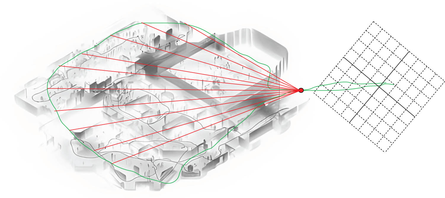
Schematic diagram of loop detection.

The state to be optimized in the map is the position and pose of intelligent hardware system of all key frames and the spatial coordinates of feature points, and all key frames and feature points in the map are represented by sum, respectively. If t i represents the position and pose of the intelligent hardware system in the i frame and l v represents the spatial coordinate of the feature point v , the state to be optimized can be expressed as

(4) x = { t i , l v } i ∈ k , v ∈ V .

The observed values of all feature points in the feature point set V in the key frame F i are denoted as Z v i = { Z i v } v ∈ V , the inertial measurement unit (IMU) measured values between two consecutive key frames are denoted as I i j = { ω k , a k } i ≤ k < j , and the estimated values of the obtained multi-sensor fusion pose in the key frame F i are denoted as Z P i = { p i , q i } i ∈ k , then the global observation information can be expressed as

(5) Z = { Z v i , I i j , Z P i } j ∈ k , v ∈ V .

Combined with the actual intelligent hardware system operation scenario, the objective function is constructed

(6) x ∗ = arg min x ∑ i ∈ k ρ ( r P i T Ω P i r P i ) + ∑ i ∈ k ρ ( r V i v T Ω V i v r V i v ) + ∑ i ∈ k ρ ( r I i j T Ω I i j r I i j ) + ∑ i ∈ k ρ ( r f i T Ω f i r f i ) ,

where r P i represents the prior residual of multi-sensor fusion pose, r V i v represents the reprojection residual of feature points, r I i j represents the IMU pre-integration residual, and r f i represents the pose plane residual. Ω P i , Ω V i v , Ω I i j , and Ω f i correspond to the covariance noise matrix of the measured values, respectively, which will be described later. ρ ( ⋅ ) is a robust kernel function, which is used to limit the gradient of the solution process and reduce the interference of external points.

As the residual of a priori estimation at key frame F i , multi-sensor fused pose is defined as the difference between the optimized pose of intelligent hardware system and the fused pose of multi-sensor. If the position estimation value of multi-sensor fusion pose in key frame F i is recorded as p i , the attitude estimation value is recorded as q i , the position of intelligent hardware system in key frame F i is recorded as p i ' , and the attitude is recorded as q i ' , the prior residual r P i of multi-sensor fusion pose can be expressed as:

(7) r P i = p i − p i ' 1 2 Δ θ T ,

where Δ θ represents the difference of the three-axis rotation angles corresponding to q i and q i ' , and the covariance matrix q i ' corresponding to Ω P i corresponds to the noise covariance of the multi-sensor fusion pose.

Feature point reprojection residual is the same as multi-state constraint Kalman filter, i.e., the difference between the observed value of spatial feature point in the image and the projection of corresponding feature point in the image. If the observation value of the feature point v in the map on the image of the key frame F i is denoted as z i v and the projection is denoted as [ u s , v s ] T , the reprojection error r V i v of the feature point v on the key frame F i is

(8) r V i v = z i v − u s v s .

The corresponding covariance matrix Ω V i v is the observation noise of vision measurement.

When the position and pose of the intelligent hardware system of the key frame F i is known, the IMU state X I i can be obtained through the external parameters of the IMU and the intelligent hardware system, and the state X I j of the key frame F _j can be calculated by integrating all IMU measurements between the key frames F i and F _j according to the IMU kinematic model

(9) q j G I = q i G I + ∫ G I q t ⊗ ω I t − b g t − n g t 0 d t P I j G = P I i G + v I i G Δ t i j + 1 2 g G Δ t i j 2 + ∬ R ( q G I ) ( a I t − b a t − n a t ) d t 2 v I j G = v I i G + g G Δ t i j + ∫ R ( q G I ) ( a I t − b a t − n a t ) d t b g j = b g i + ∫ n g d t b a j = b a i + ∫ n a d t ,

where Δ t i j represents the time interval between key frames. The relative motion estimation between the key frames can be calculated from the formula but the integration process is extremely dependent on the state of the key frame F i . When the state of F i changes in the iterative solution process, the integral needs to be recalculated. However, the data volume of IMU is much larger than that of other sensors, and repeated calculation will consume a lot of resources. Therefore, in order to avoid the problem of repeated calculation of IMU integration, IMU pre-integration method is adopted. The main idea is that the integration process is carried out in IMU coordinate system, decoupled from key frame F i , and the relative motion increment ΔI _ij independent of F i is obtained.

(10) Δ q j = 0 3 × 1 1 + ∫ Δ q t ⊗ ω I t − b g t − n g t 0 d t = q i G I ⊗ q j G I Δ p i j = ∬ Δ R i t ( q G I ) ( a I t − b a t − n a t ) d t 2 = R ( q i G I ) P I j G − P I i G − v I i G Δ t i j − 1 2 g G Δ t i j 2 v i j G = ∫ Δ R i t ( a I t − b a t − n a t ) d t = R ( q i G I ) T ( v I j G − v I j G − g G Δ t i j ) Δ b g i j = ∫ n g d t = b g j − b g i b a j = ∫ n a d t = b a j − b a i .

In practice, IMU can only provide discrete measured values. If it is assumed that the bias of the IMU at the key frame F i are b g i and b a i , and remain unchanged until the next key frame, the IMU measurements ω I k − 1 and a I k − 1 at any time k − 1 between F i and F j can be Euler integrated by the IMU pre-integrated values. That is, the pre-integration measurement Δ I i k at time u can be obtained from the pre-integration measurement Δ I i k − 1 at time k−1.

(11) Δ q i k = Δ q i k − 1 ⊗ 1 2 ( ω I k − 1 − b g t ) 0 Δ p i k = Δ p i k − 1 + Δ v i k − 1 Δ t + 1 2 Δ R i k − 1 ( a I k − 1 − b a i ) Δ t Δ v i k = Δ v i k − 1 + Δ R i k − 1 ( a I k − 1 − b a i ) Δ t Δ b g i k = 0 3 × 1 b a i k = 0 3 × 1 ,

where Δ t represents the time interval between k − 1 and k , and the initial values of IMU pre-integration are Δ q i i = [ 1 , 0 , 0 , 0 ] T , Δ p i i = 0 3 × 1 , and Δ v i i = 0 3 × 1 . From the comparison between formula (10) and IMU motion model, it can be seen that IMU pre-integrated motion model is similar to IMU motion model, except that q G I , P I G , v I G , b g t , and b a t are replaced by Δq _it, Δp _it, Δv _it, Δb _git, and Δb _ait, and gravity acceleration is removed when calculating acceleration. Therefore, the covariance transfer equation of IMU pre-integrated measurement noise between key frames F i and F j is

(12) Ω I i k = A k − 1 Ω I i k − 1 A k − 1 T + B k − 1 Ω B k − 1 B k − 1 T .

In the derivation in formula (11), it is assumed that the bias of IMU is fixed and unchanged, but it will change slightly in the actual iteration process, which will affect the change in IMU pre-integration value. At this time, it is necessary to re-integrate. Similar to IMU integration in the world coordinate system, repeated integration operation will lead to an increase in calculation amount, so the problem of repeated integration is caused by the change in IMU bias through first-order linear processing. If the update mode of IMU bias is changed as b ⌢ i + Δ b i → b i , the IMU pre-integration measurement value update process between key frames becomes

(13) Δ q i j ( b g i ) = Δ q i j ( b ⌢ g i ) ⊗ 1 2 J b g i Δ q i j Δ b g i 1 Δ p i j ( b g i , b a i ) = Δ p i j ( b ⌢ g i , b ⌢ a i ) + J b g i Δ p i j Δ b g i + J b a i Δ p i j Δ b a i Δ v i j ( b g i , b a i ) = Δ v i j ( b ⌢ g i , b ⌢ a i ) + J b g i Δ v i j Δ b g i + J b a i Δ v i j Δ b a i ,

where J x y represents the Jacobian matrix corresponding to the IMU bias of the pre-integrated measurements y against the key frame F i . From the above derivation, it can be concluded that the IMU pre-integration residuals between successive key frames F i and F j can be expressed as 15-dimensional vectors.

(14) r I i j = r Δ q i j T r Δ p i j T r Δ v i j T r Δ b b i j T r Δ b a i j T T ,

(15) r Δ q i j = Im Δ q i j ( b ⌢ g i ) ⊗ 1 2 J b g i Δ q i j Δ b g i 1 − 1 ⊗ q i G I ⊗ q j G I ,

(16) r Δ p i j = R ( q i G I ) − 1 p I j G − p I i G − v G I i Δ t i j − 1 2 g G Δ t i j 2 − ( Δ p i j ( b ⌢ g i , b ⌢ a i ) + J b g i Δ p i j Δ b g i + J b a i Δ p i j Δ b a i ) ,

(17) r Δ v i j = R ( q i G I ) − 1 ( v I j G − v I i G − g G Δ t i j ) − ( Δ v i j ( b ⌢ g i , b ⌢ a i ) + J b g i Δ v i j Δ b g i + J b a i Δ v i j Δ b a i ) ,

(18) r Δ b g i j = b g j − b g i ,

(19) r b a i j = b a j − b a i .

The moment of covariance Ω I i j is iterated by formula (12).

4 Experimental study

4.1 Experimental system

The module runs on the server, receives key frames and raster map information of single UAV through ROS distributed communication, and completes the modeling of environmental map. In the multi-machine cooperative SLAM system, a map fusion algorithm based on ORB-SLAM3-Atlas is adopted to integrate the local maps of multiple robots. ORB-SLAM 3 is a visual inertial SLAM system based on feature points, and Atlas is a strategy for processing multiple maps in ORB-SLAM 3. Among them, Atlas strategy realizes multi-machine map fusion through the following key steps.

As shown in Figure 5, first, the process of opening N sub-maps on the server, N is the number of intelligent hardware systems, and then sparse map fusion based on key frames is carried out. In the process of multi-machine cooperation, each robot generates key frames in its own local map. In order to integrate these local maps, it is necessary to identify shared key frames with the same scene information first. This can be achieved by calculating the visual bag model similarity between key frames or by local map matching.

Figure 5

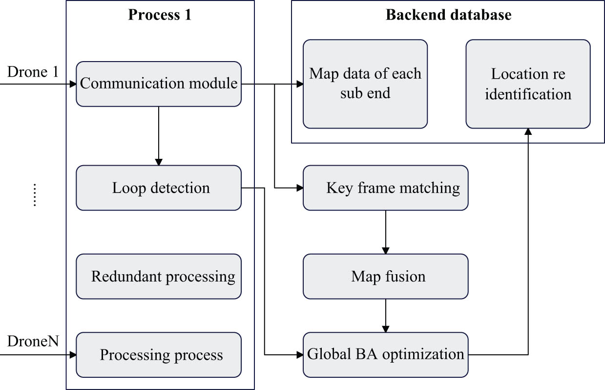
Schematic diagram of multi-map fusion.

Due to the limited computing power of a single machine, it cannot afford the task allocation of multiple machines. Therefore, the multi-machine task allocation algorithm based on frontier information is deployed on the server. As shown in Figure 6, the set exploration boundary is read from the configuration file, then the task grid is divided based on the frontier information, and then the exploration task is assigned to each sub-machine, and the single machine independently cooperates to execute the exploration task and model the environment.

Figure 6

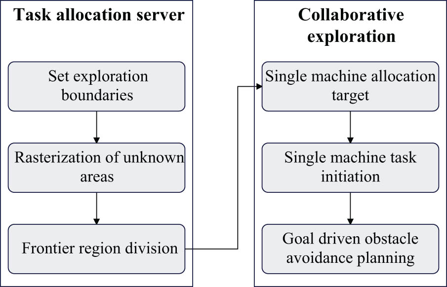
Schematic diagram of multi-machine collaborative exploration module.

4.2 Software and hardware platforms

The robot software platform used in the experiment is Ubuntu 16.04 operating system and Robot operating system (ROS). All the algorithms in this study are implemented under ROS platform, and the language used is C⁺⁺. The main function packages used in the experiment include transfer function (TF) package, rosbag function package, robot visualization (RVIZ) tool, and various open-source SLAM comparison algorithms. Among them, TF function package can conveniently realize the conversion between the coordinate systems of various sensors in the robot, rosbag function package can retain the original sensor data, which is convenient for subsequent algorithm reproduction, and RVIZ visualization tool can be used to observe the implementation effect of various SLAM algorithms in real time.

Due to the different output frequencies of sensors, the time asynchronous error of sensors is usually introduced, and the algorithm diverges when using sensor data directly to solve the data. Therefore, time synchronization of sensor data is needed. The methods of time synchronization can be divided into two categories: hardware synchronization and software synchronization. In the software design of the robot, the message_filters function package provided by ROS is used to synchronize the sensor data in time. Specifically, the TimeSynchronizer software synchronization mechanism of the message_filters function package is used, and the adaptive algorithm is used to publish the data of different sensors in approximate time stamps to reduce the time asynchronous error caused by different output frequencies of sensors. The hardware structure of the robot is shown in Figure 7.

Figure 7

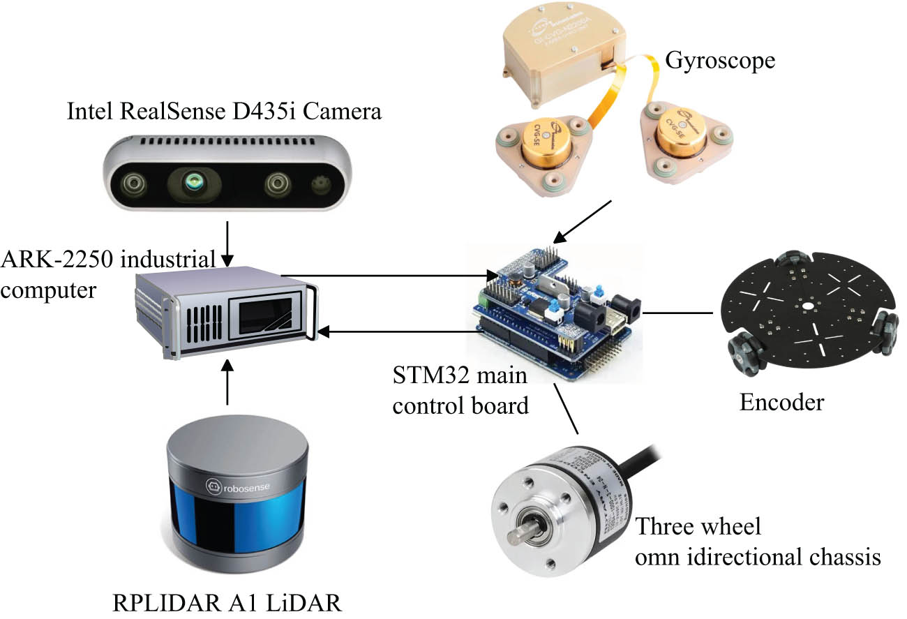
Robot hardware structure.

In this study, visual IMU is used for fusion positioning, and the accurate visual depth map generated by simulated IR structured light sensor is released to the exploration planning module as ROS topic, and the exploration module explores the environment based on hybrid global optimization.

The experimental platform collects point cloud data through Sagitar 80-line rotary lidar, as shown in Figure 8. The lidar has a detection distance of 200 m and a detection accuracy of 3 cm. It can accurately reflect the geometric mechanism of the surrounding environment, provide ROS drive, and publish point cloud data in real time under Linux system. Table 1 shows its main performance parameters.

Figure 8

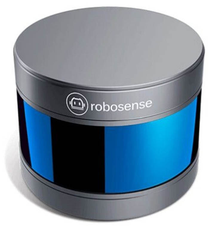
Sagitar 80-line lidar.

Table 1

Main parameters of lidar

Technical specification	Main parameters
Number of lines	80
Laser wavelength	905 nm
Blind area	≤1.0 m
Ranging capability	230 m (160 m@10% NIST)
Accuracy (typical)	Up to ±3 cm
Horizontal angle of view	360°
Vertical angle of view	40°
Horizontal angular resolution	0.2°/0.4°
Vertical angular resolution	Up to 0.1°
Frame rate	10 Hz/20 Hz

4.3 Results

This study collects laser radar data, camera data and IMU measurements in the campus environment through the unmanned vehicle experimental platform. After the data collection is completed, they are played at the same rate, and SLAM positioning and mapping experiments are carried out, respectively. In the experiment, GPS of integrated navigation system carried on unmanned vehicle is taken as the true value, and data collection is completed in sunny days, foggy days, and rainy days, respectively. By comparing the trajectories of different SLAM methods under three sets of data, and observing whether there are overlapping or unclosed phenomena in the closed loop of the built map, the positioning effect of SLAM method can be judged.

First of all, this work carries out a real vehicle experiment in sunny weather, which serves as a control group in rainy and foggy weather. The experimental route is around a large building for 1 week, and the collection time is about 9:30 am. Some sections have direct sunlight, and the overall vision is wide, with scattered pedestrians and vehicles on the road. By comparing several different algorithms, the three-dimensional trajectory of each algorithm is shown in Figure 9, in which the starting point is the origin of coordinates.

Figure 9

Comparison of SLAM three-dimensional trajectory in sunny environment. (a) The method proposed by Liu et al. [4]. (b) The method proposed by Xu et al. [5]. (c) The method proposed by Zou et al. [6]. (d) The method proposed in by Li et al. [7]. (e) The method proposed in this study.

Table 2 shows the root mean square error of SLAM accuracy, which can intuitively reflect the positioning accuracy of SLAM through data.

Table 2

SLAM trajectory evaluation

Absolute pose error (m)	RMSE
The method proposed by Zhang et al. [21]	0.6132
The method proposed by Du and Chen [22]	0.5776
The method proposed By Roggero and Diara [23]	0.3524
The method proposed by Ettefagh and Roshan Fekr [24]	4.2315
The method proposed in this work	0.3154

Next this work carries out experimental verification in rainy and foggy weather. The rainfall in the experimental environment is small to moderate, there is accumulated water on the road surface, and the fog visibility is about 60 m. Because the unmanned vehicle experimental platform is built independently, although the waterproof performance is improved by plastic film covering, it is still impossible to experiment in this environment for a long time. Therefore, the experimental route is chosen in a small square, and the route is short. Unfortunately, the initialization time of the integrated navigation system is long, and real-time kinematic analysis cannot be obtained, which leads to the erratic GPS trajectory and is inconsistent with the real environment and cannot be used. Figure 10 is a comparison diagram of SLAM three-dimensional trajectory in rain and fog environment.

Figure 10

Comparison of SLAM three-dimensional trajectories in rainy and foggy environments. (a) The method proposed by Liu et al. [4]. (b) The method proposed by Xu et al. [5]. (c) The method proposed by Zou et al. [6]. (d) The method proposed by Li et al. [7]. (e) The method proposed in this work.

To further validate the information fusion effect and system control accuracy of the model method proposed in this work, previous studies [21,22,23], and [24] as comparison objects, are used to compare the information fusion effect and system control accuracy of these models. Experiments on the MATLAB platform are conducted, through multiple sets of experiments, evaluation is done, and the obtained comparison results are shown in Table 3.

Table 3

Comparison of information fusion effect and system control accuracy

	Information fusion	Control accuracy
The method proposed by Zhang et al. [21]	90.477	79.463
The method proposed by Du and Chen [22]	89.039	83.293
The method proposed by Roggero and Diara [23]	92.154	87.353
The method proposed by Ettefagh and Roshan Fekr [24]	90.365	80.827
The method proposed in this work	98.257	96.114

4.4 Analysis and discussion

According to the research content of this work, a solid robot is built, including hardware and software. Then, this work calibrates the internal and external parameters of the sensors on the robot, and determines the coordinate transformation relationship between the sensors. Finally, this work uses the solid robot in the corridor scene and the laboratory scene to carry on the localization and the mapping experiment, respectively. Because there are many interference factors in the experiment, such as sunny days and rainy days, this work compares other open-source SLAM schemes through experimental results.

Figure 9 draws the three-dimensional trajectory graphs of each SLAM algorithm, respectively. It can be clearly seen that only the method proposed in this work can correctly complete the closed loop in three-dimensional space without obvious Z-axis offset. The closed loop of the method proposed by Liu et al. [4] is forcibly completed by the last loop detection, which shows a very unreasonable broken line in the figure, and its Z-axis offset is nearly 2 m. The Z-axis offset of the method proposed by Xu et al. [5] is 11 m, the Z-axis drift at the closed loop of the method proposed by Zou et al. [6] is 2 m, and the Z-axis offset of the method proposed by Li et al. [7] is 3 m. Therefore, it can be proved that the algorithm proposed in this work has high positioning accuracy in sunny days.

Table 3 shows the root mean square error (RMSE) of SLAM accuracy, which can intuitively reflect the positioning accuracy of SLAM through data. The algorithm proposed in this work has the smallest RMSE and the highest positioning accuracy. Compared with the method proposed by Liu et al. [4], its RMSE is reduced by 48%, and compared with the method proposed by Xu et al. [5], it is reduced by 45%, and compared with the method proposed by Zou et al. [6], it is reduced by 11%, which verifies that the accuracy of this algorithm is the highest.

Combined with the experiments in sunny days and rainy and foggy days, it can be found that the cumulative drift of the algorithm in the study by Liu et al. [4] is large. The reason is that this algorithm is a lightweight algorithm, which calculates pitch angle, roll angle and z axis of pose through ground points. Therefore, although it improves the efficiency of the algorithm, it sacrifices the accuracy. The algorithm proposed by Xu et al. [5] has high accuracy, but its loop detection effect is not good. It is difficult to achieve the expected effect in complex environment only by using Euclidean distance to judge whether the pose produces loop, which leads to certain Z-axis drift. The algorithm proposed by Zou et al. [6] performs well, and the overall accuracy is high except the trajectory Z-axis drift. However, the map size of this algorithm is fixed, which cannot save the global map in a large scene. In addition, the trajectory fluctuates violently due to the interference of rain and fog environment, which is not ideal. The algorithm proposed in this work has a good performance in both sunny days and rain and fog environment, greatly reducing the Z-axis drift of positioning, and the algorithm loop detection combined with visual word bag and point cloud matching has achieved better results without obvious cumulative error. The targeted treatment of rain and fog environment can minimize the interference of rain and fog environment, and can adapt to rain and fog environment well, which verifies the effectiveness of the algorithm.

In this work, multi-sensor fusion SLAM is studied and experimented comprehensively and systematically. The experimental results show that the algorithm proposed in this work is superior to the common open-source SLAM algorithm in positioning accuracy and mapping effect in special environment, which shows that the research results of this work meet the expectations.

From the comparison results in Table 3, it can be seen that the model proposed in this work has significant advantages in information fusion and control accuracy compared to the existing models. This verifies that the model proposed in this work has certain improvements in intelligent terminal information fusion and control accuracy.

The model in this article can improve the information fusion and control accuracy of intelligent terminals. By combining intelligent vision and other technologies, real-time control of intelligent terminals can be achieved, and automatic optimization of parameters such as action paths can be carried out according to requirements. From a practical application perspective, the model in this article is suitable for intelligent terminal devices, including but not limited to smart mobile robots used in household scenarios, such as common floor cleaning robots. Path implementation planning and optimization can be carried out according to the methods provided in this article to continuously improve their work efficiency.

The application steps of this system in reality are as follows: first, sensor calibration is carried out on the built robot platform to obtain the internal and external parameters of the relevant sensors. Then, robots are used to conduct positioning and mapping experiments in both laboratory and corridor environments. Finally, the experimental results were analyzed, which showed that the SLAM algorithm studied in this work can perform localization and mapping in complex and dynamic laboratory environments or low structure and low texture corridor scenes. Compared with common open-source SLAM algorithms, the multi-sensor fusion SLAM algorithm studied in this work has higher localization accuracy, and the generated multi-source maps can display richer environmental information.

5 Conclusion

In the process of sensor information fusion, there is not only the problem of information redundancy but also the obvious problem of time delay. For multi-sensor system, it is very important to improve the intelligent control accuracy and the timeliness of information fusion propagation. In this work, a sensor fusion algorithm combined with global optimization algorithm is proposed. According to the key frames saved in the preceding steps, feature points in local maps, sensor information and loop information, a global optimization algorithm based on graph optimization model is constructed to optimize the position and pose of intelligent hardware system and the position of spatial feature points. Moreover, this work has carried out a more comprehensive and systematic research and experiment on multi-sensor fusion SLAM. Experimental results show that the proposed algorithm is superior to the common open-source SLAM algorithm in positioning accuracy and mapping effect in special environment. Therefore, the idea of dynamic window can be considered in the follow-up research, which only optimizes locally and accelerates the operation speed. At the same time, binocular camera or depth camera can be considered in the follow-up research, which can reduce the amount of calculation and the introduction of errors.

The SLAM algorithm studied in this article did not take into account the time factor, and each part is a relatively separate module without mutual feedback, especially the globally optimized module, which takes a lot of time and cannot be performed in real time. Therefore, future research can consider introducing the idea of dynamic windows, optimizing only locally to speed up computation.

The visual sensor used in this article is a monocular RGB camera, which requires feature triangulation to obtain spatial feature point coordinates. This process requires a certain amount of computation and has certain requirements for the robot’s motion form, inevitably introducing significant errors. Therefore, future research can consider using binocular cameras or depth cameras to reduce computational complexity while also minimizing the introduction of errors.

Funding information: Authors state no funding involved.
Author contributions: All authors have accepted responsibility for the entire content of this manuscript and approved its submission.
Conflict of interest: The authors declare that they have no conflicts of interest.
Data availability statement: The data used to support the findings of the research are available from the corresponding author upon reasonable request.

References

[1] Qiu S, Zhao H, Jiang N, Wang Z, Liu L, An Y, et al. Multi-sensor information fusion based on machine learning for real applications in human activity recognition: State-of-the-art and research challenges. Inf Fusion. 2022;80:241–65.10.1016/j.inffus.2021.11.006Search in Google Scholar

[2] Liu Z, Xiao G, Liu H, Wei H. Multi-sensor measurement and data fusion. IEEE Instrum Meas Mag. 2022;25(1):28–36.10.1109/MIM.2022.9693406Search in Google Scholar

[3] Kashinath SA, Mostafa SA, Mustapha A, Mahdin H, Lim D, Mahmoud MA, et al. Review of data fusion methods for real-time and multi-sensor traffic flow analysis. IEEE Access. 2021;9:51258–76.10.1109/ACCESS.2021.3069770Search in Google Scholar

[4] Liu J, Liu Z, Zhang H, Yuan H, Manokaran KB, Maheshwari M. Multi-sensor information fusion for IoT in automated guided vehicle in smart city. Soft Comput. 2021;25:12017–29.10.1007/s00500-021-05696-3Search in Google Scholar

[5] Xu J, Yang G, Sun Y, Picek S. A multi-sensor information fusion method based on factor graph for integrated navigation system. IEEE Access. 2021;9:12044–54.10.1109/ACCESS.2021.3051715Search in Google Scholar

[6] Zou L, Wang Z, Hu J, Han QL. Moving horizon estimation meets multi-sensor information fusion: Development, opportunities and challenges. Inf Fusion. 2020;60:1–10.10.1016/j.inffus.2020.01.009Search in Google Scholar

[7] Li A, Zheng B, Li L. Intelligent transportation application and analysis for multi-sensor information fusion of Internet of Things. IEEE Sens J. 2020;21(22):25035–42.10.1109/JSEN.2020.3034911Search in Google Scholar

[8] Zhuang Y, Sun X, Li Y, Huai J, Hua L, Yang X, et al. Multi-sensor integrated navigation/positioning systems using data fusion: From analytics-based to learning-based approaches. Inf Fusion. 2023;95:62–90.10.1016/j.inffus.2023.01.025Search in Google Scholar

[9] Suseendran G, Akila D, Vijaykumar H, Jabeen TN, Nirmala R, Nayyar A. Multi-sensor information fusion for efficient smart transport vehicle tracking and positioning based on deep learning technique. J Supercomputing. 2022;78(5):6121–46.10.1007/s11227-021-04115-6Search in Google Scholar

[10] Li C, Guo S. Characteristic evaluation via multi-sensor information fusion strategy for spherical underwater robots. Inf Fusion. 2023;95:199–214.10.1016/j.inffus.2023.02.024Search in Google Scholar

[11] Muzammal M, Talat R, Sodhro AH, Pirbhulal S. A multi-sensor data fusion enabled ensemble approach for medical data from body sensor networks. Inf Fusion. 2020;53:155–64.10.1016/j.inffus.2019.06.021Search in Google Scholar

[12] Li A, Cao J, Li S, Huang Z, Wang J, Liu G. Map construction and path planning method for a mobile robot based on multi-sensor information fusion. Appl Sci. 2022;12(6):2913.10.3390/app12062913Search in Google Scholar

[13] Shifat TA, Hur JW. ANN assisted multi sensor information fusion for BLDC motor fault diagnosis. IEEE Access. 2021;9:9429–41.10.1109/ACCESS.2021.3050243Search in Google Scholar

[14] Guo Y, Fang X, Dong Z, Mi H. Research on multi-sensor information fusion and intelligent optimization algorithm and related topics of mobile robots. EURASIP J Adv Signal Process. 2021;2021:1–17.10.1186/s13634-021-00817-4Search in Google Scholar

[15] Tran MQ, Liu MK, Elsisi M. Effective multi-sensor data fusion for chatter detection in milling process. ISA Trans. 2022;125:514–27.10.1016/j.isatra.2021.07.005Search in Google Scholar PubMed

[16] Lv J, Qu C, Du S, Zhao X, Yin P, Zhao N, et al. Research on obstacle avoidance algorithm for unmanned ground vehicle based on multi-sensor information fusion. Math Biosci Eng. 2021;18(2):1022–39.10.3934/mbe.2021055Search in Google Scholar PubMed

[17] Wu L, Chen L, Hao X. Multi-sensor data fusion algorithm for indoor fire early warning based on BP neural network. Information. 2021;12(2):59.10.3390/info12020059Search in Google Scholar

[18] Zhang K, Wang Z, Guo L, Peng Y, Zheng Z. An asynchronous data fusion algorithm for target detection based on multi-sensor networks. IEEE Access. 2020;8:59511–23.10.1109/ACCESS.2020.2982682Search in Google Scholar

[19] Lin T, Wu P, Gao F. Information security of flowmeter communication network based on multi-sensor data fusion. Energy Rep. 2022;8:12643–52.10.1016/j.egyr.2022.09.072Search in Google Scholar

[20] Du H, Wang W, Xu C, Xiao R, Sun C. Real-time onboard 3D state estimation of an unmanned aerial vehicle in multi-environments using multi-sensor data fusion. Sensors. 2020;20(3):919.10.3390/s20030919Search in Google Scholar PubMed PubMed Central

[21] Zhang Y, Zhang B, Shen C, Liu H, Huang J, Tian K, et al. Review of the field environmental sensing methods based on multi-sensor information fusion technology. Int J Agric Biol Eng. 2024;17(2):1–13.Search in Google Scholar

[22] Du S, Chen S. A multi-sensor data fusion algorithm based on consistency preprocessing and adaptive weighting. Automatika. 2024;65(1):82–91.10.1080/00051144.2023.2284033Search in Google Scholar

[23] Roggero M, Diara F. Multi-Sensor 3D survey: Aerial and terrestrial data fusion and 3D modeling applied to a complex historic architecture at risk. Drones. 2024;8(4):162.10.3390/drones8040162Search in Google Scholar

[24] Ettefagh A, Roshan Fekr A. Enhancing automated lower limb rehabilitation exercise task recognition through multi-sensor data fusion in tele-rehabilitation. Biomed Eng OnLine. 2024;23(1):35.10.1186/s12938-024-01228-wSearch in Google Scholar PubMed PubMed Central

Received: 2024-06-18

Revised: 2024-08-22

Accepted: 2024-09-04

Published Online: 2024-10-25

This work is licensed under the Creative Commons Attribution 4.0 International License.

Articles in the same Issue

https://doi.org/10.1515/nleng-2024-0035

Keywords for this article

multi-sensor system; information fusion; intelligent system; SALM

Creative Commons

BY 4.0