Influence of damage on large displacement buckling analysis of beams
-
Rosalinda Arcoraci
 and
Ivo Caliò
and
Ivo Caliò

Abstract
In this study, the influence of concentrated damage on the stability of beams under static loads is investigated according to a co-rotational-based large displacement approach. Well-known benchmark beam-like structures have been considered under different loading conditions and damage scenarios. The concentrated damage has been modelled by means of a cross section reduction of a beam element, following a strategy already adopted in the literature. The results have been expressed in terms of buckling loads and post-buckling responses for different damage scenarios associated with a concentrated damage characterized by different positions, intensities, and extensions.
1 Introduction
The presence of damage can alter the static, dynamic, and stability behaviour of beam-like structures. Many authors extensively investigated the effect of single or multiple damage according to different approaches based on elastic hinges, spring models [1,2], local stiffness reduction [3,4], and finite element models (FEM) [5, 6, 7, 8, 9, 10, 11].
Among the approaches based on FEM strategies, some authors modelled the damage as a reduction in the cross-sectional area of a finite portion of the structural elements of length equal to the damage extension [5,6].
Datta et al. [7] studied the static buckling of a tapered beam with localized zones of damage and subjected to an intermediate axial load. Caddemi et al. [3] analysed the static stability of the uniform Timoshenko column in presence of multiple cracks, subjected to tensile or compressive loads. Ramana et al. [1] investigated the effects of joint flexibility, modelled as a rotational spring, on buckling analysis of free–free beams by using a finite element formulation. The influence of joint location as well as its stiffness parameters are considered. The local reduction in stiffness associated with the flexible joint can be regarded as a concentrated damage. Mohanty [8] studied the effects of a localised damage on the dynamic stability of a pre-twisted cantilever beam subjected to a time-dependent conservative axial force. The effects of parameters like pre-twist angle, extent and position of damage, and static load are investigated. Skinar [2] discussed the implementation of a simplified computational model for buckling analysis of transversely cracked beams. Jiki and Agber [9] studied the instability of a damaged pile due to a statically or dynamically applied overload using the finite element method; a damage parameter is calculated using fracture mechanics concepts. Mishra and Sahu [10] using a finite element approach investigated the influence of cracks on dynamic characteristics like free vibration, buckling, and parametric resonance characteristics of a beam with a transverse crack. Radhika and Jain [11] performed the vibration and buckling investigation of a cantilever beam produced using graphite fibre fortified polyimide with a transverse one-edge non-spreading open break utilizing the finite element strategy. Zhao [4] proposed a continuous diffused crack model to study the static stability of Euler–Bernoulli rectangular column-like structures under different boundary conditions.
The abovementioned studies consider the effect of damage under the hypothesis of linearized theory not accounting for the effects of large displacements allowing considering the post-buckling response.
The need for a geometrically nonlinear analysis becomes evident when the aim is to investigate the post-buckling behaviour of damaged structures. In fact, the presence of damage does not simply imply a linear reduction in the structural bearing capacity but introduces significant nonlinearities in deformation modes and critical buckling loads. Geometrical nonlinearities, often overlooked in conventional analyses, are crucial to fully understand how damage influences buckling. Neglecting this nonlinear component can lead to erroneous assessments and an undue underestimation of the risk of buckling in real cases.
In this study, the effects of concentrated damage on the post-buckling behaviour of beam-like structures considering large displacements have been investigated. To the author’s knowledge this is an original contribution which provides interesting insights in the geometrical nonlinear response of damaged structures. To this aim, the adopted approach, that allows taking into account geometric nonlinearities considering large displacements and rotations, is the co-rotational method well described by Crisfield in his book [12] and adopted by Yaw [13].
In particular, the co-rotational method is here applied to the evaluation of the post-buckling behaviour of some benchmark structures whose geometrically nonlinear analyses, for their healthy condition, have been already considered in the literature. The large displacement buckling response of the undamaged structures is compared with that obtained by introducing a concentrated damage. This damage has been modelled by means of a cross section reduction of a beam element with various positions, intensities, and extensions. The results proposed here, validated with literature and FEM comparison, allow highlighting the nontrivial role of concentrated damage on the post-buckling behaviour of beam-like structures.
2 Co-rotational based large displacements approach
In this study, the stability of damaged beams has been studied by means of the well-known co-rotational approach, based on the hypotheses of large displacements and rotations and small strains. The co-rotational approach allows considering geometric nonlinearities with a simple formulation and computational implementation [12,13]. Rigid body motions are differentiated from local strains by adopting two reference systems. A fixed global reference system is used to describe large displacements and rotations of the element, whereas a local element reference system, which rotates and translates with the beam element, is used to represent its small deformation.
In Figure 1, a schematic representation of the co-rotational method is reported. Precisely, C
0 denotes the original configuration of a beam element, C
R is the deformed configuration due to the rigid body motion
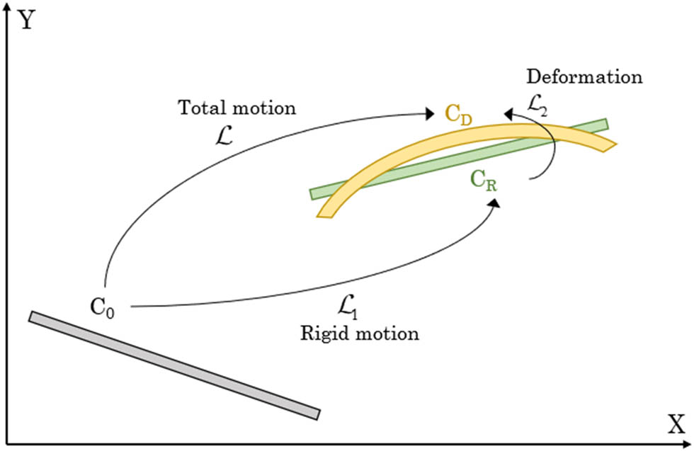
Total motion components.
Each beam is discretized in n sub-elements. The global degrees of freedom of the structure are associated with the nodal displacements and the nodal forces are dual to these displacements. The local displacements system is related to each beam element on the current configuration while the local nodal rotations represent the angles of the tangent lines at the initial and final nodes of the element with respect to the connecting line between the two nodes in the deformed configuration, denoted as θ 1l and θ 2l , Figure 2.

Initial and current configuration, due to flexural deformations, for a beam element.
In the co-rotational method, since the local reference system rotates and translates with the element, local transverse displacements are zero whereas local rotations are referred to the local reference system. Local displacements allow the direct calculation of the axial force N and the two end moments M
1 and M
2 only. Since local transverse displacements are zero, the local transverse shear forces are calculated from the end moments in the local system:
For a beam element, the local stiffness matrix is therefore given by
where EA i and EI i represent the axial and flexural stiffness of the i-th element, respectively, and L i is the original length of the i-th element.
The expression of the local stiffness matrix of a beam element k tl , after an appropriate rotation of the reference system, allows the assemblage of the global stiffness matrix of the entire structure denoted as K tl .
For the buckling analysis, it is also necessary to define the geometric stiffness matrix which allows taking into account the geometrical nonlinear contribution.
For a beam element, the geometric stiffness matrix, expressed in terms of global degrees of freedom, is given by
where
where c and s represent the cosine and sine of the angle β formed by the connecting line of nodes in the deformed configuration with respect to the horizontal direction, as shown in Figure 2.
The global geometric stiffness matrix of the entire structure K tσ is obtained by assembling the matrices of elements considering the global degrees of freedom.
Due to the geometrical nonlinearity, the relationship between forces and displacements must be formulated in the following incremental form:
where the total stiffness matrix of the structure K(u) is related to the sum of mechanical global stiffness K tl and geometrical global stiffness K tσ , ΔF is the increment of nodal forces F, and Δu the increment of nodal displacements u.
2.1 Numerical model for the damaged beam
In this study the presence of damage is modelled by introducing an element with reduced section compared to the undamaged one. This element has a cross section of the same shape of the undamaged one, but with smaller sizes, as shown in Figure 3. This model of damage allows taking into account not only the damage intensity, related to the reduction of the cross section, but also the extent of damage by means of the length of the reduced element and, when adopted in dynamic applications, considering also the mass reduction [5].

Model for the damaged beam.
The effects of different damage positions, intensities, and extension on the structural response are investigated through a parametric study.
3 Results and discussion
In this section, the buckling response of some damaged structural systems is analysed including the post-buckling behaviour. To highlight the influence of damage on buckling analysis of beam-like structures, some numerical applications with undamaged and damaged beams are presented. Specifically, the analyses include a cantilever beam subjected to axial force already studied by Lanc et al. [14] and the L-frame, known as Lee’s frame [15] studied by De Souza [16].
3.1 Cantilever beam
3.1.1 Problem overview
A cantilever beam with thin-walled cruciform cross section is shown in Figure 4. The cantilever is subjected to an axial force F applied at the free end. To activate flexural buckling mode, a transverse perturbation force of ΔF = 0.001 F is also applied as shown in Figure 4.

Cantilever beam with cruciform cross section.
The cantilever has length L = 2 m and is discretized using four equal-length beam elements and five nodes, as illustrated in Figure 5. All elements have cross section with area A = 3.16 × 10⁻⁴ m2, moment of inertia I = 3.61 × 10⁻⁸ m4 and Young’s modulus E = 1.40 × 10¹¹ N/m2.
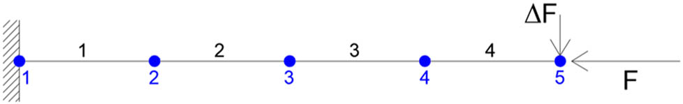
Discretization of the cantilever beam.
3.1.2 Analysis of undamaged beam
By applying the co-rotational approach for the analysis of the undamaged beam, the deformed configuration, illustrated in Figure 6, is obtained.
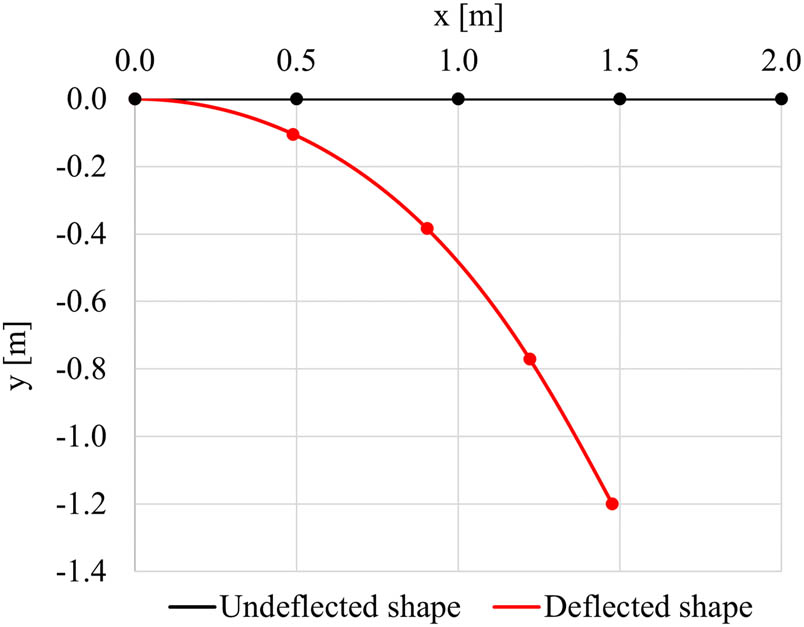
Deflected shape of the undamaged cantilever beam.
In Figure 7, the trend of the axial force F x as a function of the vertical displacement of the free end v is plotted. The vertical displacement is assumed to be positive downwards.
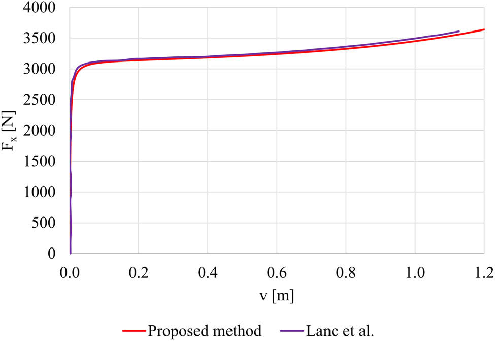
Axial load vs vertical displacement for cantilever beam.
As it can be observed, the load–displacement relationship is linear for small loads; however, as the load increases, it clearly exhibits a nonlinear behaviour, showing a hardening response. The results are compared with those of Lanc et al. [14], showing a perfect correspondence with the algorithm adopted here, implemented by the authors in a MATLAB software code [17].
3.1.3 Analysis of damaged beam
The presence of damage in the considered cantilever beam strongly modifies the response with respect to the undamaged configuration. The different behaviour is influenced by the position, intensity, as well as extent of damage, which has been initially modelled as an element with length 0.1 m and a reduced cross section height as described in the following. The influence of damage position on the structural response has been investigated by varying the location of the damaged element along the length of the beam, whereas the influence of damage intensity has been investigated by considering various reductions in cross section height. In particular, the height of the undamaged cross section equal to 0.06 m has been progressively reduced by 0.01, 0.02, 0.03, and 0.04 m, as shown in Figure 8. Two different damage positions are illustrated in Figure 9 as an example.

Damaged cross section with height reduction equal to (a) 0.01 m, (b) 0.02 m, (c) 0.03 m, and (d) 0.04 m.
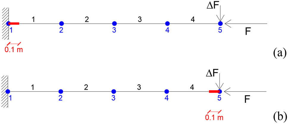
Cantilever beam with damage at (a) fixed end and (b) free end of the cantilever.
The load–displacement relationships for the considered cross section height reductions are shown in Figure 10a–d, respectively. For each damage intensity, the blue curve refers to damage located at the fixed end, whereas the green one refers to damage at the free end. For intermediate damage positions, the curves exhibit continuous variations between those reported in Figure 10. It is worth noting that a damage position at the fixed end significantly influences the response by reducing the buckling load as the damage intensity increases, whereas a damage located at the free end is quite negligible for any damage intensity, as expected. It is also useful to highlight that in this case the post-buckling behaviour maintains a stable equilibrium even in presence of damage.

Axial load vs vertical displacement for cantilever beam with damaged cross section of different heights. Blue line: damage located at the left end of beam; green line: damage located at the right end of beam. Reduction in the cross section heights of (a) 0.01 m, (b) 0.02 m, (c) 0.03 m, and (d) 0.04 m.
Since there are no available studies concerning buckling behaviour of damaged structures by means of the co-rotational approach, in order to validate the obtained results, a comparison with the outcomes acquired through the software OpenSees [18] has been performed. In particular, in both the approaches, the damage has been modelled introducing, in the beam, a reduced cross section in a certain position and for a certain extent. For the sake of brevity, only the case of damage at the fixed end of the cantilever having width 0.1 m and producing a reduction in the cross section height of 0.03 m is reported in Figure 11. The two examined curves are perfectly overlapped, showing a complete correspondence. All the other damage positions have been tested showing the same correspondence.

Axial load vs vertical displacement for cantilever beam with damaged cross section. Red solid line: results obtained with the proposed approach; black dashed line: OpenSees results. The damage is located at the left end of beam, and the reduction in the cross section height is of 0.03 m.
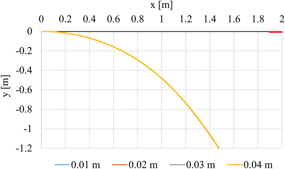
The deformed shapes for various damage intensities when the damage is located at the fixed end, mid span, and free end of the cantilever are illustrated in Figures 12–14, respectively. The position of the damaged element is indicated in the figures with a thicker red line, along the reference horizontal axis.

Deformed shape for damage at fixed end of the cantilever for cross section height reduction equal to 0.01 m (blue), 0.02 m (orange), 0.03 m (grey), and 0.04 m (yellow). The thicker red line represents the position of the damaged element.

Deformed shape for damage in the middle of the cantilever for cross section height reduction equal to 0.01 m (blue), 0.02 m (orange), 0.03 m (grey), and 0.04 m (yellow). The thicker red line represents the position of the damaged element.
Deformed shape for damage at the free end of the cantilever for cross section height reduction equal to 0.01 m (blue), 0.02 m (orange), 0.03 m (grey), and 0.04 m (yellow). The thicker red line represents the position of the damaged element.
It is interesting to point out that the presence of an element of reduced flexural stiffness introduces a relative rotation between the cross sections at the right and at the left of the damage. When the damage is located at the fixed end of the cantilever (Figure 12) and has a very high intensity, the beam rotates almost rigidly (yellow curve), confirming a result well described also by the model of a beam connected to a rotational spring, in linearised theory, for a specific value of the spring flexibility.
The curve related to the corresponding damage intensity for the damage located in the mid span of the beam (yellow line in Figure 13) clearly shows, as expected, a rigid rotation of the right side of the beam.
In Figure 14, all curves overlap because there is no damage influence when this is located at the free end of the cantilever.
In order to evaluate the influence of damage extent on the structural response, various sizes of the reduced element are analysed. In particular, the damage position is set at the fixed end of the cantilever, and the considered dimensions of the damaged element are 0.05, 0.10, and 0.15 m as shown in Figure 15.

Damage extent: (a) 0.05 m, (b) 0.10 m, and (c) 0.15 m.
Figure 16 shows the load–displacement relationship for damage located at the fixed end having variable intensity and extent. As it can be observed, the value of the critical load decreases significantly for high damage intensity and extent.

Axial load vs vertical displacement for undamaged beam (black) and damage at fixed end of the cantilever with extent equal to 0.05 m (red), 0.10 m (blue), and 0.15 m (yellow) for cross section height reduction equal to (a) 0.01 m, (b) 0.02 m, (c) 0.03 m, and (d) 0.04 m.
3.1.4 Discussion on the influence of damage position, intensity, and extent on beam behaviour
The above presented results show that, as expected, the buckling response of the damaged beam is influenced by the position, the intensity, and the extent of the damage. In Figure 17, the buckling load of the damaged cantilever F damage, normalized with respect to the corresponding value for the undamaged beam F u, is reported as a function of the damage position/length of the beam ratio (x damage/L). The buckling load gradually increases as the damage moves from the fixed to the free end, approaching the buckling load of undamaged structure. Furthermore, the buckling load decreases as the damage intensity increases. As it can be observed, the maximum reduction in the axial load is related to the damage located at the fixed end of the cantilever with highest intensity. For small damage intensities, the value of the critical load is little influenced by the damage position whereas an evident nonlinear trend can be observed for high damage intensities. The buckling load–cross section height reduction relationship, for damage located at fixed end of the cantilever, is plotted in Figure 18. The buckling load for different damage positions varies between two limit values. The upper limit represents the value of the buckling load when the cantilever beam is undamaged while the lower limit represents the buckling load value of the damaged beam with the concentrated damage at the left end, Figure 17.

Normalized buckling load as a function of the normalized damage position for undamaged (green) and damaged beam with cross section height reduction equal to 0.01 m (blue), 0.02 m (orange), 0.03 m (grey), and 0.04 m (yellow).
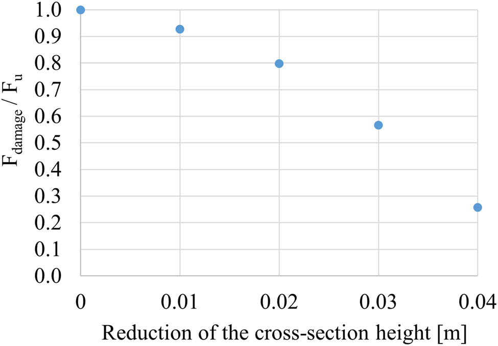
Normalized buckling load as a function of the reduction in the cross section height when the damage is at fixed end of the cantilever.
In Figure 19, the buckling load of the cantilever with damage at the fixed end, normalized with respect to the corresponding value of the undamaged beam, is reported as a function of the size of damaged element. The load gradually decreases as the dimension of the damaged element increases and as the damage intensity increases. As observed, for small reductions in the cross section height, the buckling load exhibits an almost linear decrease as the damage extent increases. However, with more significant reductions in the cross section height, the dependence becomes nonlinear.

Normalized buckling load as a function of the damage length for undamaged (black) and beam damaged at fixed end with cross section height reduction equal to 0.01 m (blue), 0.02 m (orange), 0.03 m (grey), and 0.04 m (yellow).
3.2 Lee’s frame
3.2.1 Problem overview
The second application refers to the Lee’s frame [15], as shown in Figure 20, which is a well-known benchmark studied within the geometric nonlinear analysis problems [16].

Lee’s frame: geometry and load.
The beam and column have length L = 1.2 m, rectangular cross section with area A = 6 × 10⁻⁴ m2, moment of inertia I = 2 × 10⁻⁸ m4, and Young’s modulus E = 7.06 × 10⁸ N/m2. The frame is subjected to a concentrated load applied as shown in Figure 20.
The beam and the column are discretized in sub-elements; in particular, the column is discretized using eight equal-length beam elements with length 0.15 m, while the beam is discretized with two elements with length 0.12 m on the left of the concentrated load and eight elements with length 0.12 m on the right, as depicted in Figure 21.

Discretization of Lee’s frame.
3.2.2 Analysis of undamaged frame
Figure 22 represents the load–displacement curve obtained with a geometric nonlinear analysis. The reference displacement is the vertical displacement of the node under the concentrated load. In the graph, the sign convention of De Souza [16] is adopted: forces and displacements are considered positive when directed downwards. The application of the co-rotational approach with a displacement control analysis for the undamaged frame allows obtaining the deformed configurations also, as shown in Figure 23, which correspond to the three different steps of the analysis highlighted with the coloured circles reported in Figure 22.
![Figure 22
Load–vertical displacement curve of Lee’s frame obtained with the proposed method (red) and reported in [16] (purple). The coloured circles represent the three different steps of the analysis which correspond to the deformed configurations in Figure 23.](/document/doi/10.1515/nleng-2022-0375/asset/graphic/j_nleng-2022-0375_fig_022.jpg)

Deformed shapes of Lee’s frame for the load values reported in Figure 22.
As observed in Figure 22, initially the force is positive since it is directed downwards; when the displacement increases, the force becomes negative being directed upwards. Indeed, the equilibrium path of the considered frame solution includes both snap-through and snap-back phenomena, namely, when the load decreases while the displacement increases, a snap-through behaviour occurs. Contrarily, when both load and displacement decrease simultaneously, a snap-back behaviour is observed. The results are compared with those of De Souza [16], and a perfect correspondence is observed.
3.2.3 Analysis of damaged frame
The equilibrium path of the undamaged frame, as shown in Figure 22, allows the identification of both the maximum and minimum force values obtained in the nonlinear analysis. The presence of damage in the examined structure modifies the buckling response, and consequently, the values of the maximum and minimum forces in the load–displacement curve. The damage is modelled as an element having a length of 0.03 m and a reduced cross section height. The position of this element varies along the entire frame, affecting both the column and the beam. The height of the undamaged section is equal to 0.02 m while, in order to introduce damage, a cross section height equal to 0.015 m is considered for the damaged element, as illustrated in Figure 24.
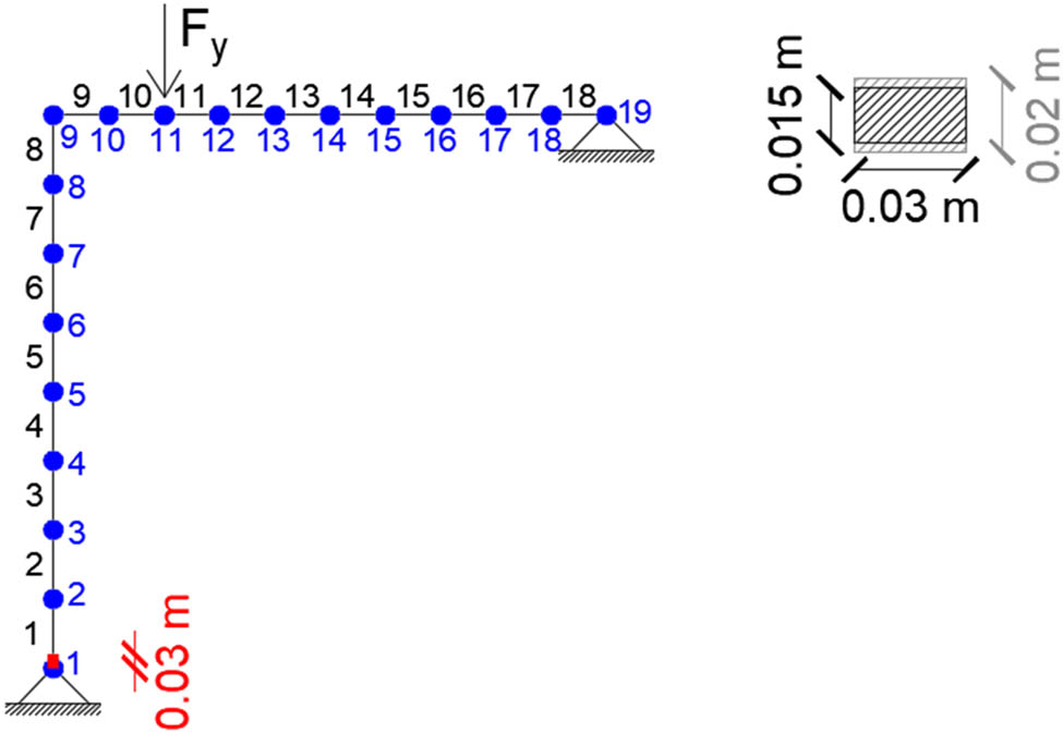
Damaged Lee’s frame and cross section geometry.
The red element in Figure 24 represents the damage and can be positioned at various locations along the column or beam. The maximum and minimum force values are calculated for different damage position along the column and beam, as shown in Figure 25.

Variation in the maximum or minimum force as a function of the damage position in the column and in the beam. (a) Variation in the maximum force as a function of the damage position in the column. (b) Variation in the maximum force as a function of the damage position in the beam. (c) Variation in the minimum force as a function of the damage position in the column. (d) Variation in the minimum force as a function of the damage position in the beam.
In Figure 25a, the variation in the maximum force as a function of the damage position in the column can be observed. When the damage is located close to the base of the column, the maximum force value remains almost the same as in the case of an undamaged frame, represented by the dashed line in Figure 25a. This result can be easily interpreted since the support at the bottom of the column already allows bending rotations which are not affected by the presence of an element of smaller stiffness. When the damage position moves upwards, a small reduction in the value of the maximum force can be first observed; then, this value increases again, and it is important to highlight that there is a range of damage positions where the maximum applied force exceeds that of the undamaged frame.
In Figure 25c, the variation in the minimum force as a function of the damage position in the column is represented. Analogous to what is observed for the maximum force, when the damage is located at the base of the column, the minimum force value remains the same as in the case of an undamaged frame, represented by the dashed line in Figure 25c. For different damage positions, the minimum force of the damaged frame always exceeds (in absolute value) that of the undamaged frame.
In Figure 25b, the variation in the maximum force as a function of the damage position along the beam can be observed. The vertical line represents the load position. When the damage is located at the right end of the beam, the maximum force value remains the same as in the case of an undamaged frame, represented by the dashed line in Figure 25b. This result is analogous to the case previously described for damage located at the bottom of the column, since the right end of the beam is hinged. For the other different damage positions, the maximum force of the damaged frame is always lower than that of the undamaged frame.
In the plot of Figure 25d, the variation in the minimum force as a function of the damage position in the beam is represented. When the damage is located at the right end of the beam, the minimum force value remains the same as in the case of an undamaged frame, represented by the dashed line in Figure 25d.
In the following, with the aim of highlighting the differences between the responses of the undamaged and damaged frame, a damaged cross section height equal to 0.01 m is considered.
Figure 26 reports the load–vertical displacement curve of two configurations of the damaged frame corresponding to a damage in the column (blue line) and in the beam (red line) compared to the undamaged configuration (black curve). The exact damage positions are specified in Figures 27 and 28 where the deformed shapes, corresponding to the three values of displacement already considered in Figure 26 (reported with coloured circles) are plotted.
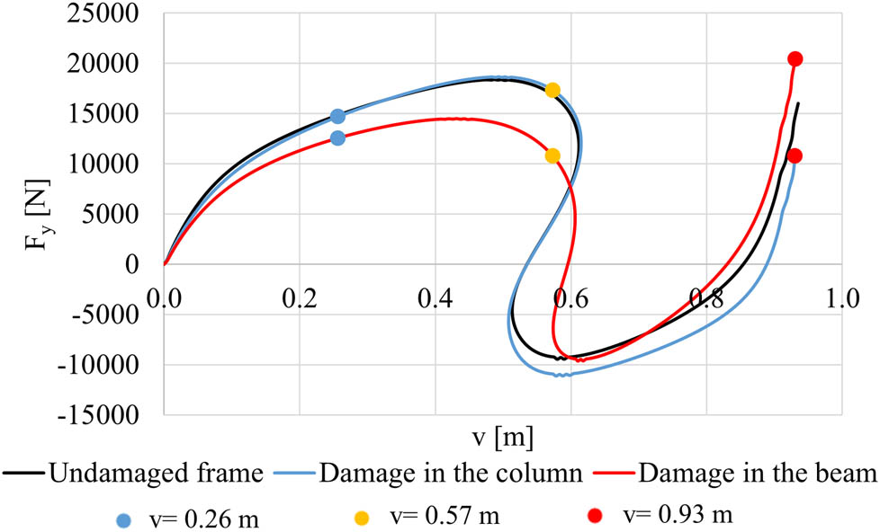
Load–vertical displacement curve of Lee’s frame for undamaged frame (black) and for damaged frame corresponding to a damage in the column (blue) and in the beam (red). The coloured circles represent the three different steps of the analysis which correspond the deformed configurations in Figures 27 and 28.

Deformed shape for undamaged Lee’s frame (grey) and for damage in the column of the frame for cross section height reduction equal to 0.01 m and for different values of vertical displacement: 0.26 m (blue), 0.57 m (yellow), and 0.93 m (red). The thicker red line represents the position of the damaged element.
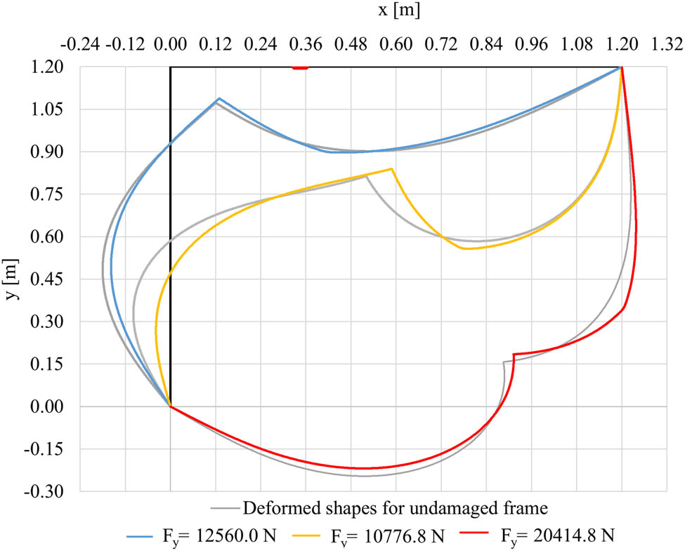
Deformed shape for undamaged Lee’s frame (grey) and for damage in the beam of the frame for cross section height reduction equal to 0.01 m and for different values of vertical displacement: 0.26 m (blue), 0.57 m (yellow), and 0.93 m (red). The thicker red line represents the position of the damaged element.
From the observation of Figure 26 different equilibrium paths in the presence of damage can be recognized. Figures 27 and 28 clearly show how the concentrated damage slightly modifies the deformed configurations corresponding to the three different investigated displacements. The presence of damage is clearly identified by a sudden change in the curvature as expected.
4 Conclusion
The proposed study presents the results of geometrically nonlinear analyses, conducted by means of the co-rotational method, on the instability of some benchmark structures in presence of concentrated damage. After analysing the undamaged structures with the aim to validate the ad hoc implemented simulation software, an original study of the effects of damage on the nonlinear behaviour of these structures has been performed.
The damage has been modelled by means of the introduction of an element of smaller flexural stiffness with respect to the undamaged one, following a strategy already applied in the literature. The presented parametric analyses consider variations in the intensity of the damage, i.e., the values of the flexural stiffness of the reduced element, location, and extent of damage.
The obtained results show that the presence of damage generally involves a reduction in the global resistance of the structures that become unstable for axial load values lower than those necessary to buckle the undamaged structure. Some interesting results have been obtained with reference to the Lee’s frame for which the presence of damage seems to provide a slightly beneficial effect in terms of applied load for some positions of the damage in the column.
The reported numerical investigations can provide useful information on the effects of damage on the large displacement buckling analysis of beam-like structures.
The implemented Matlab code will allow several future developments of the study which may concern for example the adoption of mechanical nonlinearities, different damage models and cross section variability for the structural elements.
-
Funding information: This research was funded by the Italian Ministry of University and Research (MUR) with the project no. PRIN2020 #20209F3A37.
-
Author contributions: Conceptualization: Caliò and Greco; methodology: Arcoraci and Fiore; software: Arcoraci; validation: Arcoraci and Fiore; formal analysis: all authors; writing – original draft preparation: all authors; writing – review and editing: all authors; visualization: all authors; supervision: Caliò and Greco; project administration: Caliò and Greco; and funding acquisition: Greco. All authors have read and agreed to the published version of the manuscript.
-
Conflict of interest: The authors declare no conflict of interest.
References
[1] Ramana RD, Balaram PK, Gunda J. Influence of joint flexibility on buckling analysis of free–free beams. Nonlinear Eng. 2023;12(1):20220274.10.1515/nleng-2022-0274Search in Google Scholar
[2] Skinar M. On critical buckling load estimation for slender transversely cracked beam-columns by application of a simple computational model. Comput Mater Sci. 2008;43(1):190–8.10.1016/j.commatsci.2007.07.029Search in Google Scholar
[3] Caddemi S, Caliò I, Cannizzaro F. The influence of multiple cracks on tensile and compressive buckling of shear deformable beams. Int J Solids Struct. 2013;50(20-21):3166–83.10.1016/j.ijsolstr.2013.05.023Search in Google Scholar
[4] Zhao X. Approximate analytical solution of buckling of multi damaged column like structures using a continuous difused crack model by variational iteration method. SN Appl Sci. 2021;3:39.10.1007/s42452-020-04086-ySearch in Google Scholar
[5] Caliò I, Greco A, D’Urso D. Structural models for the evaluation of eigen-properties in damaged spatial arches: a critical appraisal. Archive Appl Mech. 2016;86(11):1853–67.10.1007/s00419-016-1151-7Search in Google Scholar
[6] Caliò I, D’Urso D, Greco A. The influence of damage on the eigen-properties of Timoshenko spatial arches. Comput Struct. 2017;190:13–24.10.1016/j.compstruc.2017.04.012Search in Google Scholar
[7] Datta P, Lal M. Static stability of a tapered beam with localized damage subjected to an intermediate concentrated load. Comput Struct. 1992;43(5):971–4.10.1016/0045-7949(92)90311-MSearch in Google Scholar
[8] Mohanty S. Parametric instability of a pretwisted cantilever beam with localised damage. Int J Acoust Vib. 2007;12(4):153–61.10.20855/ijav.2007.12.4217Search in Google Scholar
[9] Jiki P, Agber J. Instability analysis of damaged pile due to static or dynamic overload. Geomaterials. 2012;2(4):114–20.10.4236/gm.2012.24016Search in Google Scholar
[10] Mishra U, Sahu S. Parametric instability of beams with transverse cracks subjected to harmonic in-plane loading. Int J Struct Stab Dyn. 2015;15(1):1540006.10.1142/S0219455415400064Search in Google Scholar
[11] Radhika S, Jain A. Buckling and vibration analysis of cracked composite beam. Int J Sci Res Dev. 2016;4(7):117–20.Search in Google Scholar
[12] Crisfield M. Non-linear Finite element analysis of solids and structures. vol. 1. Chichester, UK: John Wiley & Sons Ltd; 1991.Search in Google Scholar
[13] Yaw L. 2D Corotational Beam Formulation; 2009. [Online]. https://people.wallawalla.edu/∼louie.yaw/Co-rotational_docs/2Dcorot_beam.pdf.Search in Google Scholar
[14] Lanc D, Turkalj G, Pesic I. Global buckling analysis model for thin-walled composite laminated beam type structures. Compos Struct. 2014;111(1):371–80.10.1016/j.compstruct.2014.01.020Search in Google Scholar
[15] Lee S, Manuel Fe, Rossow E. Large deflections and stability of elastic frames. J Eng Mech. 1968;94(EM2):521–47.10.1061/JMCEA3.0000966Search in Google Scholar
[16] De Souza R. Force-based finite element for large displacement inelastic analysis of frames [dissertation]. Berkeley: University of California; 2000.Search in Google Scholar
[17] The MathWorks Inc. MATLAB version: 9.11.0 (R2021b). Natick, Massachusetts; 2021. https://www.mathworks.com.Search in Google Scholar
[18] University of California. OpenSees Command Language. Berkeley. 2006. http://opensees.berkeley.edu.Search in Google Scholar
© 2024 the author(s), published by De Gruyter
This work is licensed under the Creative Commons Attribution 4.0 International License.
Articles in the same Issue
- Editorial
- Focus on NLENG 2023 Volume 12 Issue 1
- Research Articles
- Seismic vulnerability signal analysis of low tower cable-stayed bridges method based on convolutional attention network
- Robust passivity-based nonlinear controller design for bilateral teleoperation system under variable time delay and variable load disturbance
- A physically consistent AI-based SPH emulator for computational fluid dynamics
- Asymmetrical novel hyperchaotic system with two exponential functions and an application to image encryption
- A novel framework for effective structural vulnerability assessment of tubular structures using machine learning algorithms (GA and ANN) for hybrid simulations
- Flow and irreversible mechanism of pure and hybridized non-Newtonian nanofluids through elastic surfaces with melting effects
- Stability analysis of the corruption dynamics under fractional-order interventions
- Solutions of certain initial-boundary value problems via a new extended Laplace transform
- Numerical solution of two-dimensional fractional differential equations using Laplace transform with residual power series method
- Fractional-order lead networks to avoid limit cycle in control loops with dead zone and plant servo system
- Modeling anomalous transport in fractal porous media: A study of fractional diffusion PDEs using numerical method
- Analysis of nonlinear dynamics of RC slabs under blast loads: A hybrid machine learning approach
- On theoretical and numerical analysis of fractal--fractional non-linear hybrid differential equations
- Traveling wave solutions, numerical solutions, and stability analysis of the (2+1) conformal time-fractional generalized q-deformed sinh-Gordon equation
- Influence of damage on large displacement buckling analysis of beams
- Approximate numerical procedures for the Navier–Stokes system through the generalized method of lines
- Mathematical analysis of a combustible viscoelastic material in a cylindrical channel taking into account induced electric field: A spectral approach
- A new operational matrix method to solve nonlinear fractional differential equations
- New solutions for the generalized q-deformed wave equation with q-translation symmetry
- Optimize the corrosion behaviour and mechanical properties of AISI 316 stainless steel under heat treatment and previous cold working
- Soliton dynamics of the KdV–mKdV equation using three distinct exact methods in nonlinear phenomena
- Investigation of the lubrication performance of a marine diesel engine crankshaft using a thermo-electrohydrodynamic model
- Modeling credit risk with mixed fractional Brownian motion: An application to barrier options
- Method of feature extraction of abnormal communication signal in network based on nonlinear technology
- An innovative binocular vision-based method for displacement measurement in membrane structures
- An analysis of exponential kernel fractional difference operator for delta positivity
- Novel analytic solutions of strain wave model in micro-structured solids
- Conditions for the existence of soliton solutions: An analysis of coefficients in the generalized Wu–Zhang system and generalized Sawada–Kotera model
- Scale-3 Haar wavelet-based method of fractal-fractional differential equations with power law kernel and exponential decay kernel
- Non-linear influences of track dynamic irregularities on vertical levelling loss of heavy-haul railway track geometry under cyclic loadings
- Fast analysis approach for instability problems of thin shells utilizing ANNs and a Bayesian regularization back-propagation algorithm
- Validity and error analysis of calculating matrix exponential function and vector product
- Optimizing execution time and cost while scheduling scientific workflow in edge data center with fault tolerance awareness
- Estimating the dynamics of the drinking epidemic model with control interventions: A sensitivity analysis
- Online and offline physical education quality assessment based on mobile edge computing
- Discovering optical solutions to a nonlinear Schrödinger equation and its bifurcation and chaos analysis
- New convolved Fibonacci collocation procedure for the Fitzhugh–Nagumo non-linear equation
- Study of weakly nonlinear double-diffusive magneto-convection with throughflow under concentration modulation
- Variable sampling time discrete sliding mode control for a flapping wing micro air vehicle using flapping frequency as the control input
- Error analysis of arbitrarily high-order stepping schemes for fractional integro-differential equations with weakly singular kernels
- Solitary and periodic pattern solutions for time-fractional generalized nonlinear Schrödinger equation
- An unconditionally stable numerical scheme for solving nonlinear Fisher equation
- Effect of modulated boundary on heat and mass transport of Walter-B viscoelastic fluid saturated in porous medium
- Analysis of heat mass transfer in a squeezed Carreau nanofluid flow due to a sensor surface with variable thermal conductivity
- Navigating waves: Advancing ocean dynamics through the nonlinear Schrödinger equation
- Experimental and numerical investigations into torsional-flexural behaviours of railway composite sleepers and bearers
- Novel dynamics of the fractional KFG equation through the unified and unified solver schemes with stability and multistability analysis
- Analysis of the magnetohydrodynamic effects on non-Newtonian fluid flow in an inclined non-uniform channel under long-wavelength, low-Reynolds number conditions
- Convergence analysis of non-matching finite elements for a linear monotone additive Schwarz scheme for semi-linear elliptic problems
- Global well-posedness and exponential decay estimates for semilinear Newell–Whitehead–Segel equation
- Petrov-Galerkin method for small deflections in fourth-order beam equations in civil engineering
- Solution of third-order nonlinear integro-differential equations with parallel computing for intelligent IoT and wireless networks using the Haar wavelet method
- Mathematical modeling and computational analysis of hepatitis B virus transmission using the higher-order Galerkin scheme
- Mathematical model based on nonlinear differential equations and its control algorithm
- Bifurcation and chaos: Unraveling soliton solutions in a couple fractional-order nonlinear evolution equation
- Space–time variable-order carbon nanotube model using modified Atangana–Baleanu–Caputo derivative
- Minimal universal laser network model: Synchronization, extreme events, and multistability
- Valuation of forward start option with mean reverting stock model for uncertain markets
- Geometric nonlinear analysis based on the generalized displacement control method and orthogonal iteration
- Fuzzy neural network with backpropagation for fuzzy quadratic programming problems and portfolio optimization problems
- B-spline curve theory: An overview and applications in real life
- Nonlinearity modeling for online estimation of industrial cooling fan speed subject to model uncertainties and state-dependent measurement noise
- Quantitative analysis and modeling of ride sharing behavior based on internet of vehicles
- Review Article
- Bond performance of recycled coarse aggregate concrete with rebar under freeze–thaw environment: A review
- Retraction
- Retraction of “Convolutional neural network for UAV image processing and navigation in tree plantations based on deep learning”
- Special Issue: Dynamic Engineering and Control Methods for the Nonlinear Systems - Part II
- Improved nonlinear model predictive control with inequality constraints using particle filtering for nonlinear and highly coupled dynamical systems
- Anti-control of Hopf bifurcation for a chaotic system
- Special Issue: Decision and Control in Nonlinear Systems - Part I
- Addressing target loss and actuator saturation in visual servoing of multirotors: A nonrecursive augmented dynamics control approach
- Collaborative control of multi-manipulator systems in intelligent manufacturing based on event-triggered and adaptive strategy
- Greenhouse monitoring system integrating NB-IOT technology and a cloud service framework
- Special Issue: Unleashing the Power of AI and ML in Dynamical System Research
- Computational analysis of the Covid-19 model using the continuous Galerkin–Petrov scheme
- Special Issue: Nonlinear Analysis and Design of Communication Networks for IoT Applications - Part I
- Research on the role of multi-sensor system information fusion in improving hardware control accuracy of intelligent system
- Advanced integration of IoT and AI algorithms for comprehensive smart meter data analysis in smart grids