Modeling anomalous transport in fractal porous media: A study of fractional diffusion PDEs using numerical method
-
Imtiaz Ahmad
 ,
Ibrahim Mekawy
,
Ibrahim Mekawy

Abstract
Fractional diffusion partial differential equation (PDE) models are used to describe anomalous transport phenomena in fractal porous media, where traditional diffusion models may not be applicable due to the presence of long-range dependencies and non-local behaviors. This study presents an efficient hybrid meshless method to the compute numerical solution of a two-dimensional multiterm time-fractional convection-diffusion equation. The proposed meshless method employs multiquadric-cubic radial basis functions for the spatial derivatives, and the Liouville-Caputo derivative technique is used for the time derivative portion of the model equation. The accuracy of the method is evaluated using error norms, and a comparison is made with the exact solution. The numerical results demonstrate that the suggested approach achieves better accuracy and computationally efficient performance.
1 Introduction
Numerous researchers have been exploring the application of fractional partial differential equations (FPDEs) in various scientific and technological domains in recent years. The versatility and efficacy of partial derivatives as a modeling tool have proven invaluable in capturing the historical behavior and inherent characteristics of diverse dynamic systems. Considerable efforts have been dedicated to developing numerical and analytical solutions for FPDEs [1–7]. However, many investigators have attempted to derive and simulate a variety of complicated phenomena using linear or nonlinear partial differential equations (PDEs) of integer order, but have been unsuccessful [8].
The FPDEs often encounter a diverse range of physical mechanisms. Despite the capability to represent numerous complicated phenomena in diverse fields, researchers have discovered that multiterm time-fractional PDEs, as compared to the results of a single term, enhance the modeling accuracy for characterizing diffusion processes. Nowadays, it catches the curiosity of active researchers. The objective of this work is to use a computationally appealing and trustworthy numerical technique to estimate the numerical solutions of the multiterm time-fractional convection-diffusion model equation.
The convection-diffusion PDE model holds significant physical significance and finds extensive applications in various scientific and mathematical domains. These PDEs are commonly employed in modeling biological phenomena, physical processes, and financial mathematics. Prominent examples include the Navier-Stokes equations [9], which describe fluid flow in various fields such as engineering, meteorology, and oceanography, and the well-known Burgers’ equation [10], which has applications in fluid mechanics and nonlinear waves. In addition to their relevance in physical and biological sciences, convection-diffusion models play a vital role in various environmental and energy-related studies [11–14]. For instance, these models are utilized to mathematically represent heat transport in buildings, contaminant transport in aquifers, air pollution dispersion, and groundwater flow [15]. Such applications are crucial for understanding environmental impacts, optimizing energy infrastructure, and implementing pollution control measures [16]. Moreover, many real-world phenomena involve species transportation and reaction processes that are coupled with flow processes. In the context of energy research, this is particularly significant when studying the transport and diffusion of energy-related substances or quantities [17]. Furthermore, in the field of financial mathematics and option pricing, convection-diffusion PDEs can be interpreted as probability distributions of one or more underlying stochastic processes [18–21]. This interpretation is essential for assessing and managing financial risks, especially in the context of option pricing and derivative securities.
Recent literature employs a wide range of meshless techniques to numerically address complicated PDE models in diverse fields of engineering, science, and technology. Among these methods, a prominent approach is the utilization of radial basis functions (RBFs). The meshless nature of these techniques, combined with their ability to overcome challenges associated with dimensionality, has made them increasingly popular among researchers. In addition, their versatility is enhanced by their capacity to compute solutions using uniform or non-uniform node distributions in regular and irregular domains. As a result, meshless techniques have proven to be both practical and effective in addressing various physical problems [22–28]. However, like any numerical method, meshless techniques have their limitations. Among the most significant challenges are determining the optimal shape-parameter value and handling dense, ill-conditioned matrices. To address these drawbacks, researchers have identified the local meshless technique as a favorable choice. This method exhibits accuracy and reliability in finding solutions for a wide range of integer and fractional PDE models [29,30]. Compared to the global version, the local approach yields sparse matrices that are well-conditioned and less sensitive to the choice of shape parameters. Consequently, the local meshless technique offers enhanced efficiency and benefits over its global counterpart. Due to these advantages, these methodologies are now being extensively explored and applied in various applications [31–36]. Researchers are actively utilizing meshless techniques to tackle challenging problems across different domains, demonstrating the versatility and potential of this numerical approach in advancing scientific understanding and technological innovation.
In the current research, a hybrid meshless method based on multiquadric-cubic RBF is suggested to compute the numerical solution of a two-dimensional multiterm time-fractional convection-diffusion equation, which is given as follows:
with the conditions
where the operators
where
2 Motivation
The difficulty in obtaining analytical solutions for nonlinear PDEs motivates researchers to seek efficient numerical alternatives. PDEs play a fundamental role in various real-world applications, including engineering, physics, and finance, but exact analytical solutions are often infeasible due to their nonlinearity and complexity. In response, diverse numerical approaches have been developed and evaluated, customized for specific problem characteristics and computational demands. While traditional finite difference and finite element methods are widely used, they may encounter challenges in handling irregular geometries, complex domains, and moving boundaries. In contrast, meshless methods offer an appealing alternative as they do not require a predefined mesh and efficiently handle complex geometries and unstructured domains. This adaptability makes meshless methods well suited for problems encountered in fluid dynamics, structural mechanics, and data-driven modeling. This article introduces a meshless numerical scheme for PDE models, employing RBFs for spatial derivatives and enabling accurate representation of unknown functions in higher dimensions. In addition, the temporal direction is discretized using the Caputo derivative definition. The proposed meshless approach brings several key advantages over traditional methods, including eliminating the need for a structured grid, simplifying mesh generation for complex domains, and enabling seamless extension to multidimensional problems. Furthermore, the scheme demonstrates high accuracy and numerical stability, vital for reliable and robust simulations.
2.1 Fractional calculus
Fractional derivatives are essential in fractional calculus. The following are some fundamental definitions of fractional derivatives that are commonly utilized.
Definition 1
The Riemann-Liouville derivative [38,39]
Definition 2
The Caputo’s fractional derivative [37]
Definition 3
The Atangana and Baleanu fractional derivative [40]
Definition 4
He’s fractional derivative [41]
3 Analyzing the theoretical foundations of a time discrete scheme
Initially, we present the following preliminary concepts from functional analysis, which play a crucial role in discretizing the time variable.
3.1 Introduction to applied functional analysis: A preliminary overview
Consider a bounded and open domain
The Hilbert space
using the prescribed norm in
In addition, we suppose that
In this regard, one can obtain
Next, we present the definition of the inner product within a Hilbert space.
which induces the norm
The Sobolev space
In addition, in this article, we establish the following inner product and the corresponding energy norms in
by inner products of
respectively.
Let us define
Lemma 1
Let us suppose
and
Proof
Sun and Wu [42].
Lemma 2
Let
Proof
Directly follows from Lemma 1.
Lemma 3
Let
Proof
Sun and Wu [42].
4 Spatial and temporal discretization techniques for derivatives
In this section, we present the main steps involved in computing the spatial and temporal derivatives. These steps are essential for the accurate numerical approximation.
4.1 Spatial discretization techniques for derivatives
The derivatives of
Procedure for one-dimensional case is
where the hybrid RBF is defined as
The matrix representation of Eqs (9) and (10) is
where
Matrix notation of Eq. (11) is
where
The matrix
The derivative of
Matrix notation of Eq. (14) is
or
The approximate semi-discretized form for model (1), using hybrid meshless method, along with the initial and boundary conditions, is
In this context, the matrix
4.2 Numerical approaches for time derivatives discretization
The time derivative in the Caputo form, denoted as
Taking into account
where
Then,
Let
5 Results and discussion
The recommended hybrid meshless method is examined in this section for its application and accuracy in estimating the numerical solution of the two-dimensional multiterm time-fractional convection-diffusion model equation. Different time fractional orders, including two-term, three-term, and five-term, are taken into consideration. The method is coupled with multiquadric-cubic radial basis functions, and rectangular and nonrectangular domains have been taken into consideration. The temporal step size
where
Problem 1
The exact solution for Eq. (1) with
The required numerical results for Problem 1 are produced using the suggested hybrid meshless approach and are shown in Table 1. The nodes
Results of the hybrid meshless method for Problem 1
|
|
|
|
|||||
|---|---|---|---|---|---|---|---|
|
|
RMS | MaxE | RMS | MaxE | RMS | MaxE | |
| Two-term | 0.1 |
|
|
|
|
|
|
| 0.05 |
|
|
|
|
|
|
|
| 0.01 |
|
|
|
|
|
|
|
| 0.005 |
|
|
|
|
|
|
|
| 0.001 |
|
|
|
|
|
|
|
| Three-term | 0.1 |
|
|
|
|
|
|
| 0.05 |
|
|
|
|
|
|
|
| 0.01 |
|
|
|
|
|
|
|
| 0.005 |
|
|
|
|
|
|
|
| 0.001 |
|
|
|
|
|
|
|
| Five-term | 0.1 |
|
|
|
|
|
|
| 0.05 |
|
|
|
|
|
|
|
| 0.01 |
|
|
|
|
|
|
|
| 0.005 |
|
|
|
|
|
|
|
| 0.001 |
|
|
|
|
|
|
|
In Table 2, the numerical results are obtained using a range of fractional-order and final time
Results of the hybrid meshless method for Problem 1
| Two-term | Three-term | Five-term | |||||
|---|---|---|---|---|---|---|---|
|
|
RMS | MaxE | RMS | MaxE | RMS | MaxE | |
|
|
0.2 |
|
|
|
|
|
|
| 0.5 |
|
|
|
|
|
|
|
| 1 |
|
|
|
|
|
|
|
|
|
0.2 |
|
|
|
|
|
|
| 0.5 |
|
|
|
|
|
|
|
| 1 |
|
|
|
|
|
|
|
|
|
0.2 |
|
|
|
|
|
|
| 0.5 |
|
|
|
|
|
|
|
| 1 |
|
|
|
|
|
|
|

Results in terms of RMS error of the hybrid meshless method for Problem 1.
The ease of implementation in the irregular domain is one of the key benefits of meshless approaches over mesh-based techniques. The three non-rectangular domain types that are considered in this article are shown in Figures 2, 4, and 5. We have display the numerical results in Figure 3 for
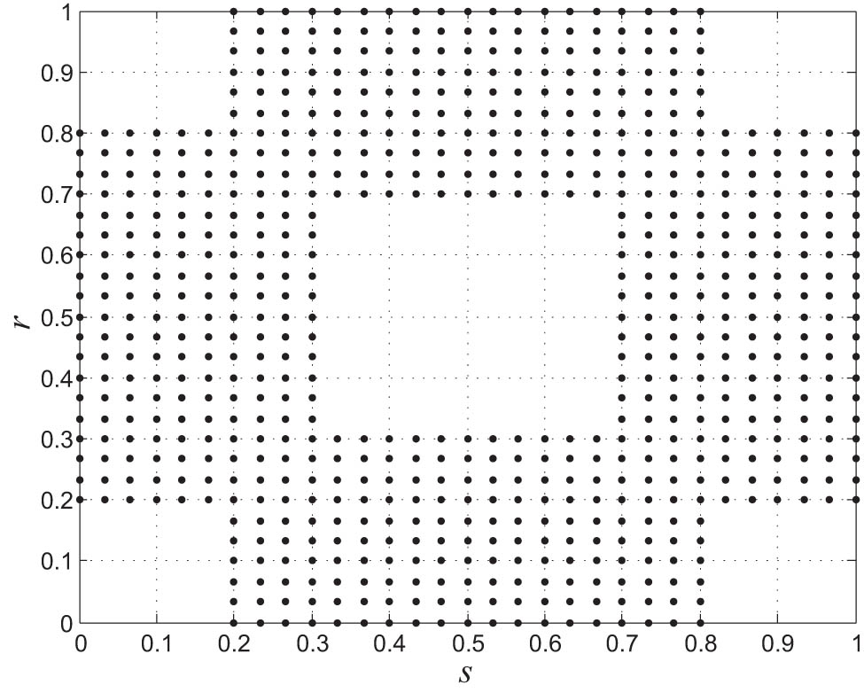
Computational domain.

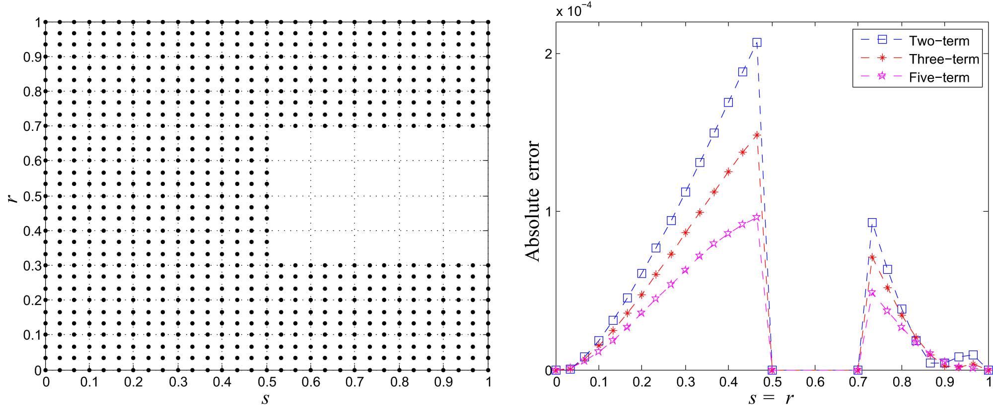
The computational domain and results of the hybrid meshless method for Problem 1.
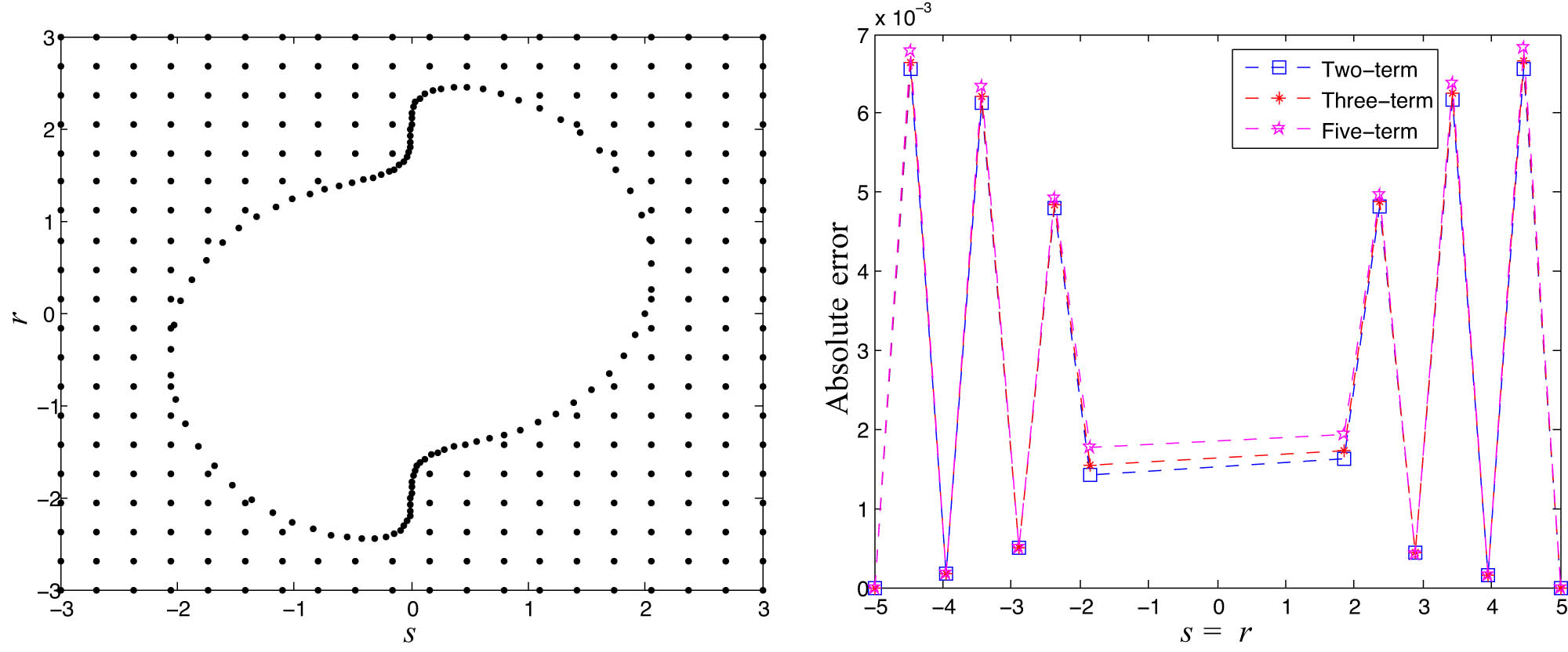
The computational domain and results of the hybrid meshless method for Problem 1.
Problem 2
As a second test problem, the exact solution for Eq. (1) with
The numerical results, the suggested hybrid meshless approach for Problem 2 are shown in Table 3. The nodes
Results of the hybrid meshless method for Problem 2
|
|
|
|
|||||
|---|---|---|---|---|---|---|---|
|
|
RMS | MaxE | RMS | MaxE | RMS | MaxE | |
| Two-term | 0.05 |
|
|
|
|
|
|
| 0.01 |
|
|
|
|
|
|
|
| 0.005 |
|
|
|
|
|
|
|
| 0.001 |
|
|
|
|
|
|
|
| Three-term | 0.05 |
|
|
|
|
|
|
| 0.01 |
|
|
|
|
|
|
|
| 0.005 |
|
|
|
|
|
|
|
| 0.001 |
|
|
|
|
|
|
|
| Five-term | 0.05 |
|
|
|
|
|
|
| 0.01 |
|
|
|
|
|
|
|
| 0.005 |
|
|
|
|
|
|
|
| 0.001 |
|
|
|
|
|
|
|
Results of the hybrid meshless method for Problem 2
| Two-term | Three-term | Five-term | |||||
|---|---|---|---|---|---|---|---|
|
|
RMS | MaxE | RMS | MaxE | RMS | MaxE | |
|
|
1 |
|
|
|
|
|
|
| 2 |
|
|
|
|
|
|
|
|
|
1 |
|
|
|
|
|
|
| 2 |
|
|
|
|
|
|
|
|
|
1 |
|
|
|
|
|
|
| 2 |
|
|
|
|
|
|
|
6 Conclusion
In this article, we have effectively solved the multiterm fractional-order convection-diffusion equation with the hybrid meshless method. Numerical studies were carried out for different values of time-fractional order
Acknowledgments
Researchers would like to thank the Deanship of Scientific Research, Qassim University for funding publication of this project.
-
Author contributions: All authors have accepted responsibility for the entire content of this manuscript and approved its submission.
-
Conflict of interest: The authors declare no conflict of interest.
-
Ethics approval and consent to participate: All authors demonstrate adherence to accepted ethical standards for genuine research. As corresponding author, I have obtained consent from all authors for their participation in this study.
-
Consent to publish: All the authors are agreed to publish this research work.
-
Data availability statement: Data will be provided on request to the corresponding author.
References
[1] Ahmad H, Khan TA, Ahmad I, Stanimirović PS, Chu YM. A new analyzing technique for nonlinear time fractional Cauchy reaction-diffusion model equations. Results Phys. 2020;19:103462. 10.1016/j.rinp.2020.103462Search in Google Scholar
[2] Inc M, Khan MN, Ahmad I, Yao SW, Ahmad H, Thounthong P. Analysing time-fractional exotic options via efficient local meshless method. Results Phys. 2020;19:103385. 10.1016/j.rinp.2020.103385Search in Google Scholar
[3] Mahreen K, Ain QT, Rahman G, Abdalla B, Shah K, Abdeljawad T. Approximate solution for the nonlinear fractional order mathematical model. AIMS Math. 2022;7(10):19267–86. 10.3934/math.20221057Search in Google Scholar
[4] Arfan M, Mahariq I, Shah K, Abdeljawad T, Laouini G, Mohammed PO. Numerical computations and theoretical investigations of a dynamical system with fractional order derivative. Alex Eng J. 2022;61(3):1982–94. 10.1016/j.aej.2021.07.014Search in Google Scholar
[5] Rehman ZR, Boulaaras S, Jan R, Ahmad I, Bahramand S. Computational analysis of financial system through non-integer derivative. J Comput Sci. 2023;75:102204. 10.1016/j.jocs.2023.102204. Search in Google Scholar
[6] Shah NNH, Jan R, Ahmad H, Razak NNA, Ahmad I, Ahmad H. Enhancing public health strategies for tungiasis: A mathematical approach with fractional derivative. AIMS Bioeng. 2023;10(4):384–405. 10.3934/bioeng.2023023Search in Google Scholar
[7] Ain QT, Anjum N, Din A, Zeb A, Djilali S, Khan ZA. On the analysis of Caputo fractional order dynamics of middle east lungs coronavirus (MERS-CoV) model. Alex Eng J. 2022;61(7):5123–31. 10.1016/j.aej.2021.10.016Search in Google Scholar
[8] Rizvi STR, Afzal I, Ali K. Chirped optical solitons for Triki-Biswas equation. Mod Phys Lett B. 2019;33(22):1950264. 10.1142/S0217984919502646Search in Google Scholar
[9] McLean D. Understanding aerodynamics: Arguing from the real physics. Hoboken (NJ), USA: John Wiley and Sons; 2012. 10.1002/9781118454190Search in Google Scholar
[10] Burgers JM. A mathematical model illustrating the theory of turbulence. Adv Appl Mech. 1948;1:171–99. 10.1016/S0065-2156(08)70100-5Search in Google Scholar
[11] Ahmad I, Riaz M, Ayaz M, Arif M, Islam S, Kumam P. Numerical simulation of partial differential equations via local meshless method. Symmetry. 2019;11(2):257. 10.3390/sym11020257Search in Google Scholar
[12] Ahmad I, Ahsan M, Din ZU, Masood A, Kumam P. An efficient local formulation for time-dependent PDEs. Mathematics. 2019;7(3):216. 10.3390/math7030216Search in Google Scholar
[13] Ahmad I, Ahsan M, Hussain I, Kumam P, Kumam W. Numerical simulation of PDEs by local meshless differential quadrature collocation method. Symmetry. 2019 11(3):394. 10.3390/sym11030394Search in Google Scholar
[14] Wang F, Zhang J, Ahmad I, Farooq A, Ahmad H. A novel meshfree strategy for a viscous wave equation with variable coefficients. Front Phys. 2021;9:701512. 10.3389/fphy.2021.701512Search in Google Scholar
[15] Jalghaf HK, Kovács E, Bolló B. Comparison of old and new stable explicit methods for heat conduction, convection, and radiation in an insulated wall with thermal bridging. Buildings. 2022;12(9):1365. 10.3390/buildings12091365Search in Google Scholar
[16] Li DS. Convection-diffusion modeling for chemical pollutant dispersion in the joint of artificial lake using finite element method. Bulg Chem Commun. 2015;47:949–58. Search in Google Scholar
[17] Khan H, Mustafa S, Ali I, Kumam P, Baleanu D, Arif M. Approximate analytical fractional view of convection-diffusion equations. Open Phys. 2020;18(1):897–905. 10.1515/phys-2020-0184Search in Google Scholar
[18] Safdari-Vaighani A, Heryudono A, Larsson E. A radial basis function partition of unity collocation method for convection-diffusion equations arising in financial applications. J Sci Comput. 2015;64(2):341–67. 10.1007/s10915-014-9935-9Search in Google Scholar
[19] Ain QT, Wan J. A stochastic analysis of co-infection model in a finite carrying capacity population. Int J Biomath. 2023;2350083. 10.1142/S1793524523500833Search in Google Scholar
[20] Mohammed PO, Alqudah MA, Hamed YS, Kashuri A, Abualnaja KM. Solving the modified regularized long wave equations via higher degree B-spline algorithm. J Funct Space. 2021;1–10. 10.1155/2021/5580687Search in Google Scholar
[21] Ain QT, Nadeem M, Karim S, Akguuul A, Jarad F. Optimal variational iteration method for parametric boundary value problem. AIMS Math. 2022;7(9):16649–56. 10.3934/math.2022912Search in Google Scholar
[22] Thounthong P, Khan MN, Hussain I, Ahmad I, Kumam P. Symmetric radial basis function method for simulation of elliptic partial differential equations. Mathematics. 2018;6(12):327. 10.3390/math6120327Search in Google Scholar
[23] Wang F, Hou E, Ahmad I, Ahmad H, Gu Y. An efficient meshless method for hyperbolic telegraph equations in (1+1) dimensions. CMES-Comp. Model Eng Sci. 2021;128(2):687–98. 10.32604/cmes.2021.014739Search in Google Scholar
[24] Mehnaz S, Khan MN, Ahmad I, Abdel-Khalek S, Alghamdi AM, Inc M. The generalized time fractional Gardner equation via numerical meshless collocation method. Therm Sci. 2022;26(1):469–74. 10.2298/TSCI22S1469MSearch in Google Scholar
[25] Ain QT, He JH, Anjum N, Ali M. The fractional complex transform: A novel approach to the time-fractional Schrödinger equation. Fractals. 2020;28(7):2050141. 10.1142/S0218348X20501418Search in Google Scholar
[26] Khan Z, Srivastava HM, Mohammed PO, Jawad M, Jan R, Nonlaopon K. Thermal boundary layer analysis of MHD nanofluids across a thin needle using non-linear thermal radiation. Math Biosci Eng. 2022;19(12):14116–41. 10.3934/mbe.2022658Search in Google Scholar PubMed
[27] Srivastava HM, Gusu DM, Mohammed PO, Wedajo G, Nonlaopon K, Hamed YS. Solutions of general fractional-order differential equations by using the spectral tau method. Fractal Fract. 2021;6(1):7. 10.3390/fractalfract6010007Search in Google Scholar
[28] Jan A, Srivastava HM, Khan A, Mohammed PO, Jan R, Hamed YS. In vivo HIV dynamics, modeling the interaction of HIV and immune system via non-integer derivatives. Fractal Fract. 2023;7(5):361. 10.3390/fractalfract7050361Search in Google Scholar
[29] Ahmad I, Ahmad H, Inc M, Yao SW, Almohsen B. Application of local meshless method for the solution of two term time fractional-order multi-dimensional PDE arising in heat and mass transfer. Therm Sci. 2020;24(1):95–105. 10.2298/TSCI20S1095ASearch in Google Scholar
[30] Ahmad I, Khan MN, Inc M, Ahmad H, Nisar KS. Numerical simulation of simulate an anomalous solute transport model via local meshless method. Alex Eng J. 2020;59(4):2827–38. 10.1016/j.aej.2020.06.029Search in Google Scholar
[31] Wang F, Khan MN, Ahmad I, Ahmad H, Abu-Zinadah H, Chu YM. Numerical solution of traveling waves in chemical kinetics: time-fractional Fishers equations. Fractals. 2022;30(02):2240051. 10.1142/S0218348X22400515Search in Google Scholar
[32] Ahmad I, Ali I, Jan R, Idris SA, Mousa M. Solutions of a three-dimensional multiterm fractional anomalous solute transport model for contamination in groundwater. PloS One. 2023;18(12):e0294348. 10.1371/journal.pone.0294348Search in Google Scholar PubMed PubMed Central
[33] Ahmad I, Bakar AA, Ali I, Haq S, Yussof S, Ali AH. Computational analysis of time-fractional models in energy infrastructure applications. Alex Eng J. 2023;82:426–36. 10.1016/j.aej.2023.09.057Search in Google Scholar
[34] Ahmad H, Khan MN, Ahmad I, Omri M, Alotaibi MF. A meshless method for numerical solutions of linear and nonlinear time-fractional Black-Scholes models. AIMS Math. 2023;8(8):19677–98. 10.3934/math.20231003Search in Google Scholar
[35] Li JF, Ahmad I, Ahmad H, Shah D, Chu YM, Thounthong P, et al. Numerical solution of two-term time-fractional PDE models arising in mathematical physics using local meshless method. Open Phys. 2020;18(1):1063–72. 10.1515/phys-2020-0222Search in Google Scholar
[36] Wang F, Ahmad I, Ahmad H, Alsulami MD, Alimgeer KS, Cesarano C, et al. Meshless method based on RBFs for solving three-dimensional multiterm time fractional PDEs arising in engineering phenomenons. J King Saud Univ Sci. 2021;33(8):101604. 10.1016/j.jksus.2021.101604Search in Google Scholar
[37] Caputo M. Linear models of dissipation whose Q is almost frequency independent-II. Geophys J Int. 1967;13(5):529–39. 10.1111/j.1365-246X.1967.tb02303.xSearch in Google Scholar
[38] Jumarie G. Stock exchange fractional dynamics defined as fractional exponential growth driven by (usual) Gaussian white noise. Application to fractional Black-Scholes equations. Insur Math Econ. 2008;42(1):271–87. 10.1016/j.insmatheco.2007.03.001Search in Google Scholar
[39] Jumarie G. Derivation and solutions of some fractional Black-Scholes equations in coarse-grained space and time. Application to Merton’s optimal portfolio. Comput Math Appl. 2010;59(3):1142–64. 10.1016/j.camwa.2009.05.015Search in Google Scholar
[40] Atangana A, Baleanu D. New fractional derivatives with non-local and nonsingular kernel theory and application to heat transfer model. Therm Sci. 2016;20:763. 10.2298/TSCI160111018ASearch in Google Scholar
[41] He JH. A new fractal derivation. Therm Sci. 2011;15(1):145–7. 10.2298/TSCI11S1145HSearch in Google Scholar
[42] Sun ZZ, Wu X. A fully discrete difference scheme for a diffusion-wave system. Appl Numer Math. 2006;56(2):193–209. 10.1016/j.apnum.2005.03.003Search in Google Scholar
[43] Sarra S. A local radial basis function method for advection-diffusion-reaction equations on complexly shaped domains. Appl Math Comput. 2012;218(19):9853–65. 10.1016/j.amc.2012.03.062Search in Google Scholar
© 2024 the author(s), published by De Gruyter
This work is licensed under the Creative Commons Attribution 4.0 International License.
Articles in the same Issue
- Editorial
- Focus on NLENG 2023 Volume 12 Issue 1
- Research Articles
- Seismic vulnerability signal analysis of low tower cable-stayed bridges method based on convolutional attention network
- Robust passivity-based nonlinear controller design for bilateral teleoperation system under variable time delay and variable load disturbance
- A physically consistent AI-based SPH emulator for computational fluid dynamics
- Asymmetrical novel hyperchaotic system with two exponential functions and an application to image encryption
- A novel framework for effective structural vulnerability assessment of tubular structures using machine learning algorithms (GA and ANN) for hybrid simulations
- Flow and irreversible mechanism of pure and hybridized non-Newtonian nanofluids through elastic surfaces with melting effects
- Stability analysis of the corruption dynamics under fractional-order interventions
- Solutions of certain initial-boundary value problems via a new extended Laplace transform
- Numerical solution of two-dimensional fractional differential equations using Laplace transform with residual power series method
- Fractional-order lead networks to avoid limit cycle in control loops with dead zone and plant servo system
- Modeling anomalous transport in fractal porous media: A study of fractional diffusion PDEs using numerical method
- Analysis of nonlinear dynamics of RC slabs under blast loads: A hybrid machine learning approach
- On theoretical and numerical analysis of fractal--fractional non-linear hybrid differential equations
- Traveling wave solutions, numerical solutions, and stability analysis of the (2+1) conformal time-fractional generalized q-deformed sinh-Gordon equation
- Influence of damage on large displacement buckling analysis of beams
- Approximate numerical procedures for the Navier–Stokes system through the generalized method of lines
- Mathematical analysis of a combustible viscoelastic material in a cylindrical channel taking into account induced electric field: A spectral approach
- A new operational matrix method to solve nonlinear fractional differential equations
- New solutions for the generalized q-deformed wave equation with q-translation symmetry
- Optimize the corrosion behaviour and mechanical properties of AISI 316 stainless steel under heat treatment and previous cold working
- Soliton dynamics of the KdV–mKdV equation using three distinct exact methods in nonlinear phenomena
- Investigation of the lubrication performance of a marine diesel engine crankshaft using a thermo-electrohydrodynamic model
- Modeling credit risk with mixed fractional Brownian motion: An application to barrier options
- Method of feature extraction of abnormal communication signal in network based on nonlinear technology
- An innovative binocular vision-based method for displacement measurement in membrane structures
- An analysis of exponential kernel fractional difference operator for delta positivity
- Novel analytic solutions of strain wave model in micro-structured solids
- Conditions for the existence of soliton solutions: An analysis of coefficients in the generalized Wu–Zhang system and generalized Sawada–Kotera model
- Scale-3 Haar wavelet-based method of fractal-fractional differential equations with power law kernel and exponential decay kernel
- Non-linear influences of track dynamic irregularities on vertical levelling loss of heavy-haul railway track geometry under cyclic loadings
- Fast analysis approach for instability problems of thin shells utilizing ANNs and a Bayesian regularization back-propagation algorithm
- Validity and error analysis of calculating matrix exponential function and vector product
- Optimizing execution time and cost while scheduling scientific workflow in edge data center with fault tolerance awareness
- Estimating the dynamics of the drinking epidemic model with control interventions: A sensitivity analysis
- Online and offline physical education quality assessment based on mobile edge computing
- Discovering optical solutions to a nonlinear Schrödinger equation and its bifurcation and chaos analysis
- New convolved Fibonacci collocation procedure for the Fitzhugh–Nagumo non-linear equation
- Study of weakly nonlinear double-diffusive magneto-convection with throughflow under concentration modulation
- Variable sampling time discrete sliding mode control for a flapping wing micro air vehicle using flapping frequency as the control input
- Error analysis of arbitrarily high-order stepping schemes for fractional integro-differential equations with weakly singular kernels
- Solitary and periodic pattern solutions for time-fractional generalized nonlinear Schrödinger equation
- An unconditionally stable numerical scheme for solving nonlinear Fisher equation
- Effect of modulated boundary on heat and mass transport of Walter-B viscoelastic fluid saturated in porous medium
- Analysis of heat mass transfer in a squeezed Carreau nanofluid flow due to a sensor surface with variable thermal conductivity
- Navigating waves: Advancing ocean dynamics through the nonlinear Schrödinger equation
- Experimental and numerical investigations into torsional-flexural behaviours of railway composite sleepers and bearers
- Novel dynamics of the fractional KFG equation through the unified and unified solver schemes with stability and multistability analysis
- Analysis of the magnetohydrodynamic effects on non-Newtonian fluid flow in an inclined non-uniform channel under long-wavelength, low-Reynolds number conditions
- Convergence analysis of non-matching finite elements for a linear monotone additive Schwarz scheme for semi-linear elliptic problems
- Global well-posedness and exponential decay estimates for semilinear Newell–Whitehead–Segel equation
- Petrov-Galerkin method for small deflections in fourth-order beam equations in civil engineering
- Solution of third-order nonlinear integro-differential equations with parallel computing for intelligent IoT and wireless networks using the Haar wavelet method
- Mathematical modeling and computational analysis of hepatitis B virus transmission using the higher-order Galerkin scheme
- Mathematical model based on nonlinear differential equations and its control algorithm
- Bifurcation and chaos: Unraveling soliton solutions in a couple fractional-order nonlinear evolution equation
- Space–time variable-order carbon nanotube model using modified Atangana–Baleanu–Caputo derivative
- Minimal universal laser network model: Synchronization, extreme events, and multistability
- Valuation of forward start option with mean reverting stock model for uncertain markets
- Geometric nonlinear analysis based on the generalized displacement control method and orthogonal iteration
- Fuzzy neural network with backpropagation for fuzzy quadratic programming problems and portfolio optimization problems
- B-spline curve theory: An overview and applications in real life
- Nonlinearity modeling for online estimation of industrial cooling fan speed subject to model uncertainties and state-dependent measurement noise
- Quantitative analysis and modeling of ride sharing behavior based on internet of vehicles
- Review Article
- Bond performance of recycled coarse aggregate concrete with rebar under freeze–thaw environment: A review
- Retraction
- Retraction of “Convolutional neural network for UAV image processing and navigation in tree plantations based on deep learning”
- Special Issue: Dynamic Engineering and Control Methods for the Nonlinear Systems - Part II
- Improved nonlinear model predictive control with inequality constraints using particle filtering for nonlinear and highly coupled dynamical systems
- Anti-control of Hopf bifurcation for a chaotic system
- Special Issue: Decision and Control in Nonlinear Systems - Part I
- Addressing target loss and actuator saturation in visual servoing of multirotors: A nonrecursive augmented dynamics control approach
- Collaborative control of multi-manipulator systems in intelligent manufacturing based on event-triggered and adaptive strategy
- Greenhouse monitoring system integrating NB-IOT technology and a cloud service framework
- Special Issue: Unleashing the Power of AI and ML in Dynamical System Research
- Computational analysis of the Covid-19 model using the continuous Galerkin–Petrov scheme
- Special Issue: Nonlinear Analysis and Design of Communication Networks for IoT Applications - Part I
- Research on the role of multi-sensor system information fusion in improving hardware control accuracy of intelligent system
- Advanced integration of IoT and AI algorithms for comprehensive smart meter data analysis in smart grids