Addressing target loss and actuator saturation in visual servoing of multirotors: A nonrecursive augmented dynamics control approach
-
Archit Krishna Kamath


Abstract
Traditional position and image-based visual servoing techniques often pose challenges in terms of target loss and actuator saturation. These challenges arise due to the requirement of calculating inverse Jacobians to determine robot motions and the susceptibility of these methods to image noise. To address the aforementioned challenges, this article presents a nonrecursive augmented dynamics control (NRADC) that establishes a direct correlation between variations in image pixels and the thrust and torque commands of a multirotor. By incorporating pixel variations into the dynamics of the multirotor, this approach enables the utilization of state constraints to address the issue of target loss. In addition, the correlation between image pixels and control commands allows for the integration of image noise with system uncertainties. Consequently, a single controller can be designed to simultaneously handle both aspects while considering input constraints, effectively addressing the problem of actuator saturation. Notably, unlike conventional control approaches that handle input and state constraints, the proposed NRADC approach is nonrecursive, making it well suited for implementation on systems with limited on-board computational resources, such as multirotors. The effectiveness of the proposed method is demonstrated through experimental validations, including a performance comparison with a nonrecursive controller from recent literature.
1 Introduction
With the exponential advancement in integrated circuits and manufacturing technology, minicomputers have evolved to efficiently pack increased computing resources while conserving energy. This progress enables the execution of intricate image processing tasks on hand-held devices, eliminating the need for the large GPU setups that were prevalent in the past. Consequently, researchers globally have directed their efforts towards developing efficient visual servoing algorithms capable of handling complex tasks, including object recognition, object tracking, pick-and-place maneuvers, and precision docking applications. The burgeoning trends in the visual servoing domain hold significant promise, particularly for multirotor unmanned aerial systems. Their unique capabilities, such as vertical take-off and landing, precise hovering, and agile maneuvering, position them as ideal candidates for visually guided tasks. Applications span diverse fields, encompassing search and rescue operations, drug delivery, condition monitoring, and reporting systems [1–3]. Existing position and image-based visual servoing algorithms rely on the computation of inverse Jacobians to determine the multirotor’s motion, making them computationally expensive and highly susceptible to image noise [4–6]. Moreover, these algorithms do not directly tackle the issues of target loss and actuator saturation.
Recent research has explored the combination of conventional visual servoing with machine learning algorithms to tackle target loss [5,7]. However, these approaches are recursive in nature and primarily applicable when the object of interest is already outside the camera’s line of sight during tracking. They do not actively contribute to keeping the object within the camera’s field of view. Furthermore, in the existing literature, actuator saturation is treated separately from its application to visual servoing, resulting in the need for two distinct solutions and increasing the computational burden on the multirotor’s onboard computer. To overcome these limitations, this article introduces a nonrecursive augmented dynamics control (NRADC) approach for visual servoing. This approach incorporates pixel variations into the multirotor’s dynamics, establishing a direct relationship between pixel variation and the multirotor’s thrust and torque commands. This correlation enables the modelling of target loss as a state constraint problem and the addressing of actuator saturation as an input constraint control problem. However, an additional challenge remains: the development of a nonrecursive robust controller to complement the augmented dynamics, capable of handling both input and state constraint issues effectively.
Previous studies have addressed input constraints using anti-windup controllers, but these approaches neglect state constraints and are vulnerable to system uncertainties and disturbances [8,9]. Model predictive control (MPC) strategies have been proposed to handle both input and state constraints, but their recursive nature makes them computationally expensive and lacking in robustness [10]. To enhance robustness, some studies propose combining an integral sliding mode controller with a linear MPC algorithm or utilizing a receding horizon-based discrete sliding mode algorithm [11,12]. However, these approaches remain recursive.
In the domain of sliding mode control, a second-order sliding mode controller has been demonstrated to be effective in handling systems with output constraints [13]. This approach incorporates a barrier Lyapunov function and a power integrator term to ensure the system’s output stays within predefined boundaries. However, it does not consider input constraints. Conversely, a chattering-free sliding mode control law based on unidirectional auxiliary surfaces has been introduced to handle state constraints [14]. Nevertheless, this work does not account for input constraints and primarily focuses on limiting the rate of change of the state rather than the state itself.
The limitations mentioned earlier are addressed in a study [15] that deals with a second-order system subject to both input and state constraints. The proposed algorithm divides the operational region into two zones with fixed control effort values corresponding to the maximum allowable input constraint. However, this approach results in significant chattering in the control channel, leading to frequent actuator saturation and instability in systems utilizing camera-based indoor localization. An extension of this algorithm to higher-order systems is presented in [16], where a higher-order sliding mode controller is proposed to mitigate chattering. Nonetheless, the inclusion of integrator chains makes the system sluggish and susceptible to integral windup.
Based on the findings of Rubagotti and Ferrara [15] and Incremona et al. [16], the proposed NRADC approach is inspired. This approach incorporates a nonrecursive terminal sliding mode controller with a power rate reaching law to address systems with input and state constraints [17,18]. The main contributions of this study are as follows:
Development of an augmented dynamics multirotor model that integrates pixel variations into the dynamics of the multirotor. This model establishes a correlation between pixel accelerations and the thrust and torque commands of the multirotor.
Formulation of a nonrecursive robust control law based on a terminal sliding mode controller with a power rate reaching law. This controller is designed to handle systems with both input and state constraints.
Development of a controller gain tuning algorithm to ensure the convergence of error trajectories within a desired boundary of the sliding manifold while strictly adhering to input and state constraints.
Real-time validation of the proposed NRADC approach in preventing target loss and actuator saturation in a target tracking task.
This article is organized as follows: Sections 2 and 3 present the augmented dynamics visual servoing model and outline the problem formulation. Controller design and implementation procedures are addressed in Sections 4 and 5, respectively. Sections 6 and 7 provide details on numerical simulations and experimental validations, respectively followed by concluding remarks in Section 8.
2 Mathematical model
This section presents the details pertaining to the development of the augmented multirotor dynamics for a 6DoF multirotor by extending the idea presented by Kamath et al. [19].
2.1 Multirotor’s dynamical model
The 6-degree-of-freedom multirotor model necessitates 12 states to depict its motion in three-dimensional space. The equation of motion for the multirotor can be expressed through state space representation, as depicted below [20].
where:
- (2)
To obtain the thrust input of the multirotor and the inner loop desired values of the roll and pitch angle, (2) is used as follows:
2.2 Acceleration image dynamics
This subsection presents the acceleration image dynamics. To understand this, consider a 3D point
where
In a situation where the 3D point,
where
where
where
where
(1) and (8) can be combined to obtain the augmented dynamical model.
2.3 Augmented dynamical multirotor model
In order to derive the augmented dynamical model of the multirotor, the outer loop state variables of the multirotor are employed. This approach is taken to ensure the effective tracking of POIs using the multirotor UAV. Consequently, the dynamics considered for augmentation are extracted from (1) and are presented as follows:
Since pixel acceleration in (8) is a for 2D pixel values and the outer loop dynamics of the multirotor has three variables, the relationship between them will have to be obtained by splitting the outer loop dynamics into two subsections as shown:
where the subscripts dep and pos represent the depth and the position subsystem, respectively. For instance, if the camera setup is as depicted in Figure 1, the dep parameter would align with the

Multirotor and camera setup.
The augmented dynamical model can be obtained using the pos subsystem alongside (8). To relate the variables of (8) with that of (11), a rotation matrix
Substituting (12) in (8) and eliminating the zero columns:
where
For ease of representation, (13) can be rewritten as follows:
where
Therefore, the outer loop control is now split into two subsystems: the depth subsystem and the augmented dynamics position subsystem. The state of the multirotor in each of these subsystems is influenced by the camera’s orientation in relation to the multirotor.
Remark 1
The transformed bounded disturbance vector, i.e.,
Remark 2
The following assumptions are made for this work: The intrinsic parameters of the camera being used are fully known. Uncertainties in the depth estimations and intrinsic parameters are assumed to be minimal. A LiDAR is employed in conjunction with the monocular camera to facilitate the acquisition of depth.
3 Problem formulation
Consider the complete augmented dynamics multirotor model obtained from (1) and (16):
Let the aforementioned dynamics be subjected to a set of state constraints
Considering the imposed constraints, the following conditions hold:
Remark 3
The constraint
4 Control strategy design
Consider a nonlinear system represented by the equation:
where
This effectively implies that the functions
where
where
Sets
To derive the control effort
This nonlinear sliding manifold ensures that the state trajectories converge to zero in finite time
where
4.1 Stability analysis
The stability analysis begins with establishing that the control effort
Theorem 1
For the given nonlinear system described in (20), when subjected to the control effort defined in (25), it can be proven that the system will converge to a small neighborhood in the vicinity of the sliding manifold specified by (24) within a finite time interval
Proof
Considering a positive definite Lyapunov candidate function
Simplifying the aforementioned equation further, we obtain
To further simplify the aforementioned inequality, three cases are considered:
Based on the analysis of the three aforementioned cases, it can be concluded that
Solving the aforementioned differential equation, the convergence time can be obtained using the expression [23]:
On similar lines, the power rate reaching law can also prove to be finite-time convergent by substituting
Since,
The following part of this section is dedicated to proving that the control algorithm effectively confines the system states within the desired state constraints.
Theorem 2
When applying the control law
Proof
Consider the region
Noting that points
Consider the scenario when
In the case of
4.2 Control parameter tuning
To limit the magnitude of the control effort
where
The aforementioned inequality is in terms of
Fixing speed of convergence: If the convergence speed is fixed, the value of
(34)Based on the stability analysis presented earlier, the gain
(35)Fixing
Fixing the region of convergence: If the region of convergence around the sliding manifold is fixed, it implies fixing the value of
In both methods, one of the control law parameters needs to be selected heuristically, while the other is determined based on the input and state constraints. To illustrate the implementation of the proposed controller.
4.3 Implementation example
To demonstrate the effectiveness of the controller, consider the nonlinear second order system:
where
For

Regulation task results. (a)
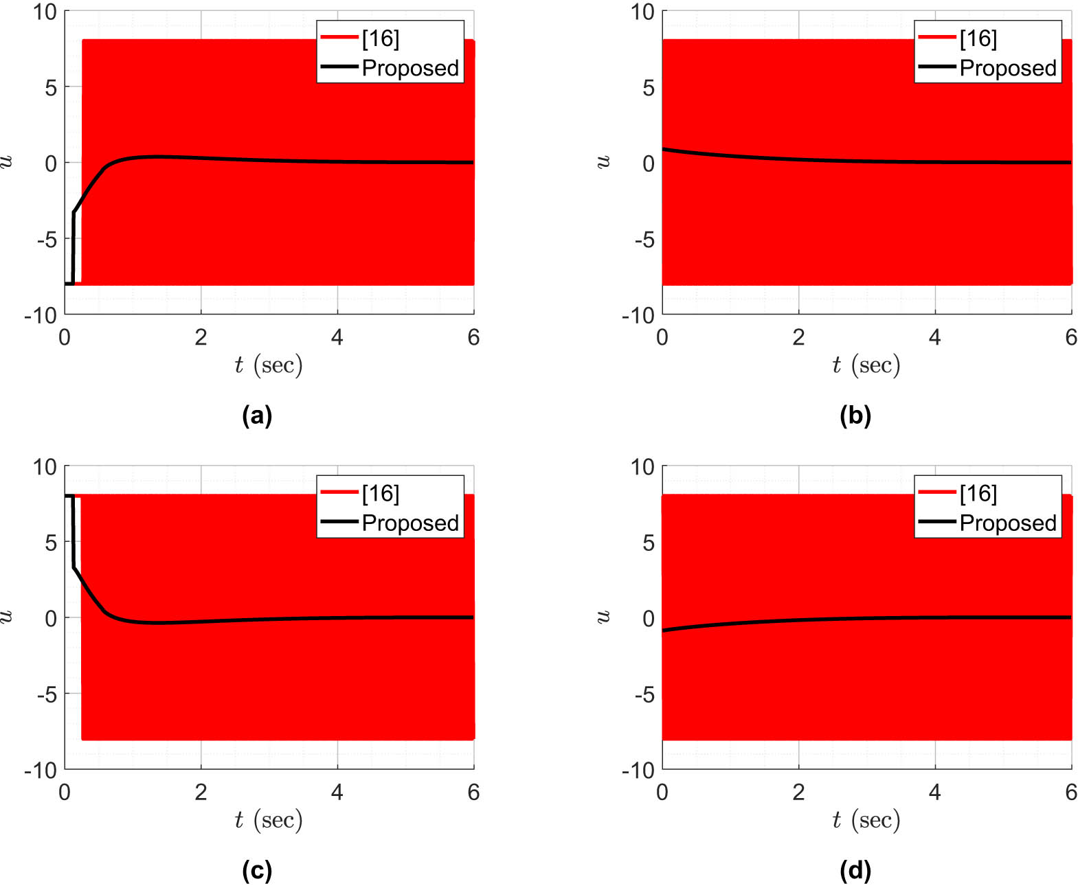
Control efforts. (a)
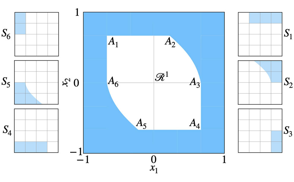
Figure 3 represents the phase plot for the system with different initial conditions,
The control effort profile for both the controllers is presented in Figure 4. The controller in [15] produce significant chattering to stabilize the system states to (0, 0) as opposed to the proposed controller. To mathematically assess the performance of the proposed controller with respect to the study by Rubagotti and Ferrara [15], integral square error (ISE), integral absolute error (IAE), integral time absolute error (ITAE), average control effort (ACE), average value of control effort between samples (
Performance evaluation
| Index | Formula | Proposed | [15] |
|---|---|---|---|
| ISE |
|
0.4374 | 0.4386 |
| IAE |
|
0.5714 | 0.8317 |
| ITAE |
|
0.3461 | 1.1068 |
| ACE |
|
0.6467 | 2.8261 |
|
|
|
0.3797 | 14.9131 |
| DOC |
|
0.5871 | 5.2770 |
From the entries of Table 1, one can see that the convergence error, to the origin, is smaller in the case of the proposed controller, as opposed to [15]. In addition, the DOC and the average control effort between samples are also lesser in case of the proposed controller. Similar performance indices can be observed for different values of
5 Control implementation
Since the objective of the problem formulation was to develop a control strategy for converging the states to a desired value rather than the origin, it is necessary to convert the state model in (17) into error dynamics to accommodate this control strategy. The state errors can be defined as follows:
For (38), the state constraints
where
By considering the constraints
The value of
6 Numerical simulations
In this section, the numerical simulations for the proposed approach are presented. The system parameters selected for simulation are detailed in Table 2. It is noteworthy that the value of
Simulation parameters
| Parameters | Value | Parameters | Value |
|---|---|---|---|
| m | 0.5 kg | g |
|
|
|
0.0075 kg m
|
|
0.0075 kg
|
|
|
0.0150 kg m
|
|
0.1 cm |
|
|
57/53 |
|
0.75 |
Distinct values are assigned to the controller gain
The subsequent subsection presents the results of the regulation and tracking tasks for three cases, specifically:
Case 1: The system is influenced by a conventional terminal sliding mode controller with a power rate reaching law and no constraints.
Case 2: The system is influenced by a conventional terminal sliding mode controller with a power rate reaching law and input saturation only.
Case 3: The system, under the influence of the proposed controller, is subjected to both input and state constraints.
In each scenario, it is assumed that the system is exposed to a bounded lumped disturbance (comprising system uncertainties, external disturbances, and image noises) with magnitudes
6.1 Regulation task
The goal of the regulation task is to transition the multirotor from the initial pixel coordinates

Augmented outer loop states.

Inner loop states.
Analyzing Figure 5 and Table 5, it is evident that the time constants for the responses of
Time constant comparison
| State | Time constant (sec) | ||
|---|---|---|---|
| Case 1 | Case 2 | Case 3 | |
|
|
0.62 | 0.64 | 0.71 |
|
|
0.62 | 0.64 | 0.71 |
|
|
0.91 | 0.91 | 0.91 |
|
|
0.82 | 0.82 | 0.82 |
Tables 3 and 4 detail the maximum values of system states and control effort in both cases. Examination of these tables reveals that the maximum values of system states are considerably higher in Cases 1 and 2 compared to Case 3, especially in states governing the system’s velocity. This observation implies that the addition of input saturation may not effectively constrain the system states to lower values and could potentially contribute to system instability.
Comparison table of state variables
| Task | Case | Parameters | |||||||||||
|---|---|---|---|---|---|---|---|---|---|---|---|---|---|
|
|
|
|
|
|
|
|
|
|
|
|
|
||
| Regulation | Case 1 | 2 | 0.3 | 0.2 | 0.68 | 0.79 | 0.5 | 0.96 | 0.28 | 0.28 | 6.93 | 7.7 | 0.53 |
| Case 2 | 2 | 0.3 | 0.2 | 0.15 | 0.21 | 0.5 | 0.96 | 0.28 | 0.28 | 4.81 | 4.18 | 0.53 | |
| Case 3 | 2 | 0.3 | 0.2 | 0.12 | 0.13 | 0.5 | 0.96 | 0.19 | 0.19 | 0.5 | 0.5 | 0.53 | |
| Tracking | Case 1 | 2 | 0.3 | 0.2 | 1.2 | 0.2 | 0.5 | 0.96 | 0.22 | 0.25 | 12.5 | 1.32 | 0.53 |
| Case 2 | 2 | 0.3 | 0.2 | 0.27 | 0.28 | 0.5 | 0.96 | 0.22 | 0.25 | 5.69 | 3.64 | 0.53 | |
| Case 3 | 2 | 0.3 | 0.2 | 0.19 | 0.19 | 0.5 | 0.96 | 0.19 | 0.19 | 0.5 | 0.5 | 0.49 | |
Comparison table of control effort
| Task | Case | Parameters | |||||
|---|---|---|---|---|---|---|---|
|
|
|
|
|
|
|
||
| Regulation | Case 1 | 35.2 | 35.2 | 16 | 2.82 | 4.91 | 0.19 |
| Case 2 | 15 | 15 | 15 | 1 | 1 | 0.19 | |
| Case 3 | 15 | 15 | 15 | 1 | 1 | 0.19 | |
| Tracking | Case 1 | 24.4 | 33.9 | 16 | 6.85 | 0.86 | 0.19 |
| Case 2 | 15 | 15 | 15 | 1 | 0.86 | 0.19 | |
| Case 3 | 15 | 15 | 15 | 1 | 0.86 | 0.19 | |
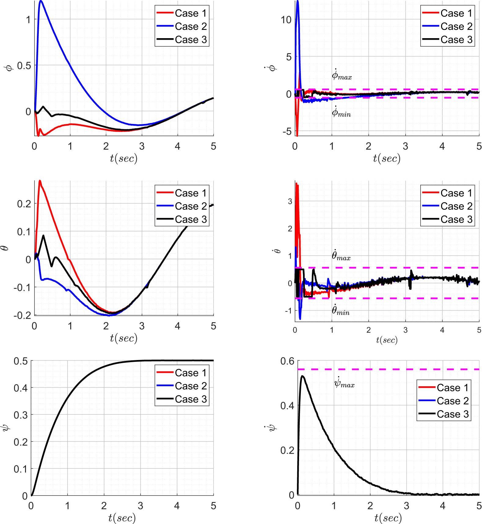
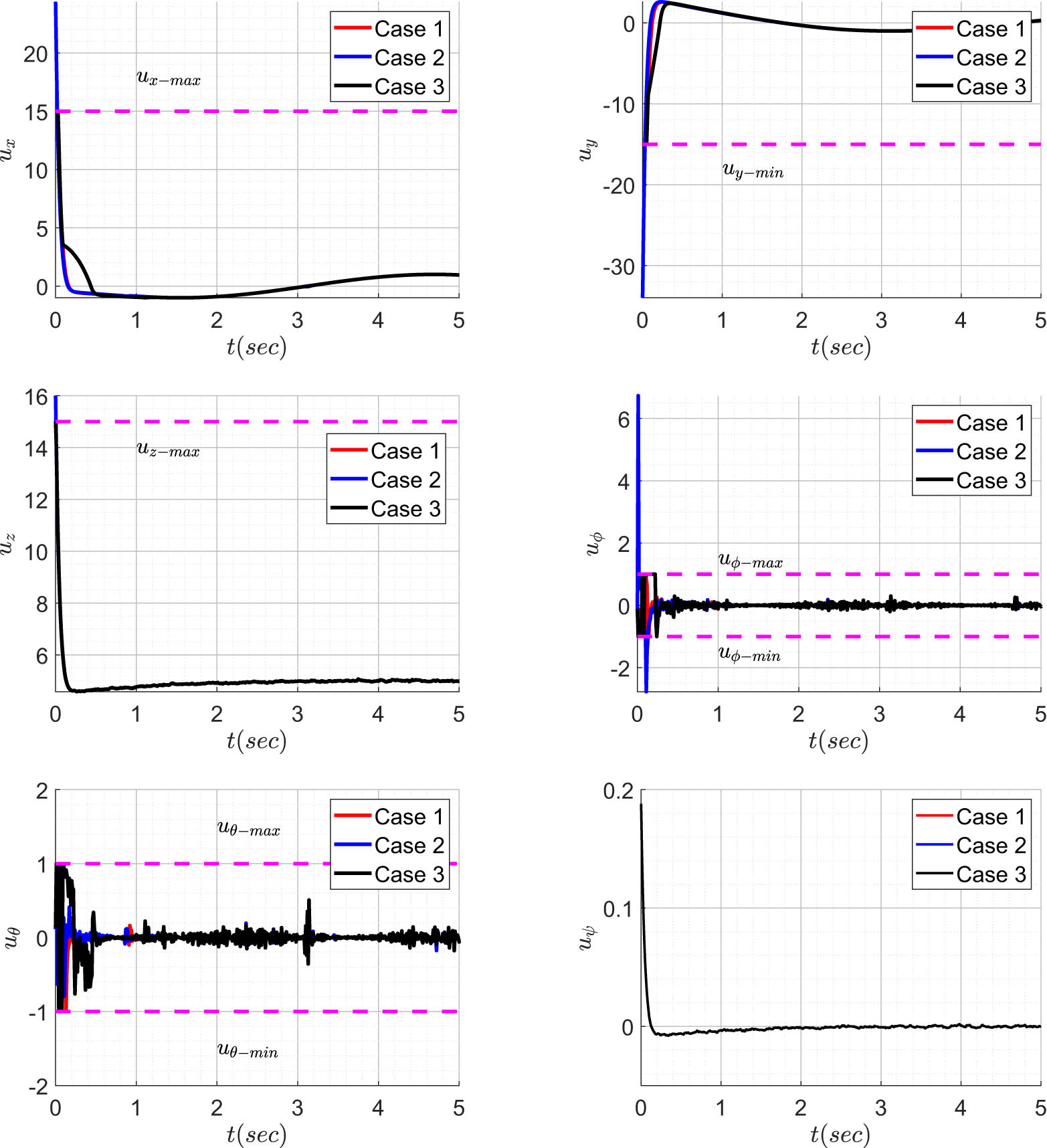
A similar pattern is evident in the inner loop states, as depicted in Figure 6. It is noteworthy that the proposed controller restricts the inner loop variables to values significantly lower than the original behaviour, in contrast to Cases 1 and 2. This is particularly significant since a high rate of change in attitude dynamics can induce erratic motions in the system, ultimately leading to instability. In Figure 7, the control effort is presented in the presence and absence of the input constraints

Control effort.
6.2 Tracking task
In the tracking task, the multirotor is tasked with pursuing a point undergoing circular motion. This is translated into sinusoidal pixel motion characterized by a magnitude of 0.1 and a frequency of 0.15 rad/s. Adjustments to altitude and yaw align with the parameters established in the preceding task. Subsequently, the tracking results for cases 1, 2, and 3 will be graphically illustrated using blue, red, and black representations, respectively.
Figures 8 and 9 illustrate the system states during the tracking task for the three considered cases, while Tables 3 and 4 outline the absolute maximum values of both system states and control efforts, as previously conducted. Similar to the regulation task, as observed in Figures 8 and 9, it is evident that the proposed controller (Case 3) effectively performs the tracking task, closely aligning its response with that of Cases 1 and 2. Despite the previously mentioned response sluggishness, its impact on the tracking behaviour of the system is minimal to negligible.

Augmented outer loop states.
Inner loop states.
The proposed controller’s significance (Case 3) becomes apparent when examining the velocity states of the system. This is evident in the data presented in Table 3 and illustrated in Figures 8 and 9. In Cases 1 and 2, the rate of change in states, particularly the inner loop states, is notably higher than that in Case 3. In addition, the velocity magnitudes exhibit erratic changes in Cases 1 and 2 compared to the more stable behaviour observed in Case 3. This stability is crucial in visual servoing applications, particularly when dealing with dynamic targets. Abrupt increases in system velocities (linear and/or angular) in Cases 1 and 2 may lead to unpredictable movements, potentially causing the system to lose sight of the target being tracked.
As depicted in Figure 10 and corroborated by the data in Table 4, the magnitude of control effort is significantly reduced. This reduction holds potential to alleviate issues related to electronic speed controllers overheating and, concurrently, contribute to an extended flight time. The succeeding section presents the experimental validation of the proposed approach on a real-time hardware for a tracking task.
Control effort.
7 Experimental validation
The proposed approach’s effectiveness is validated by conducting experiments on a quadrotor system, depicted in Figure 11. The quadrotor is built using a DJI F450 frame and includes a carbon fibre landing gear to improve shock absorption during landings. To automate the quadrotor’s flight, the Holybro Pixhawk RPi CM4 Baseboard is utilized as the flight controller. This hardware platform combines the functionalities of the Raspberry Pi Compute Module 4 and the Pixhawk autopilot system. For visual perception, a Logitech BRIO 500 camera is mounted on the quadrotor, facing downwards. This camera has a 4K ultra-high-definition sensor, allowing for the capture of clear and sharp images even in low-light conditions. In addition, to enhance depth estimation, a LiDAR sensor is used in conjunction with the downward-facing camera, operating within the same reference frame.

Hardware setup.
An automatic ground vehicle (AGV) equipped with an ArUco marker is employed to accomplish target tracking. Figure 12 visually depicts the three-dimensional trajectory followed by the quadrotor as it tracks the AGV on the ground. This experiment aims to simulate various scenarios, such as target loss and actuator saturation, by directing the AGV to follow a lemniscate trajectory at different velocities. The proposed NRADC’s effectiveness is assessed and compared to the performance of the nonrecursive controller outlined by Rubagotti and Ferrara [15] alongside the augmented multirotor dynamics within each of these scenarios.

3D trajectory of quadrotor tracking the AGV using NRADC approach.
The controller is configured with
In this task, the AGV maintains a constant speed of 1 m/s, while the quadrotor takes off from the AGV and ascends to an altitude of 4 m. Once reaching this altitude, the NRADC algorithm for tracking is activated. The objective of the quadrotor is to continuously track the target along a lemniscate trajectory while adhering to the system’s constraints. Box and whisker plots for the variations in system states and inputs during the tracking process at a speed of 1 m/s are shown in Figures 13 and 14. These plots demonstrate the effectiveness of the proposed NRADC in maintaining both steady-state values (represented by the boxes) and transient values (represented by the whiskers) of the system states and inputs within the specified constraints. Table 6 provides the average control effort (ACE), the average value of control effort between samples (

Quadrotor’s augmented dynamical state variables (left) and altitude and inner loop state variables (right).

Quadrotor’s auxiliary outer loop (left) and inner loop (right) control efforts.
Performance evaluation for the control effort
| Index | Formula | Proposed | [15] |
|---|---|---|---|
| ACE |
|
0.6467 | 2.8261 |
|
|
|
0.3797 | 14.9131 |
| DOC |
|
0.5871 | 5.2770 |
The results mentioned earlier can be reproduced when tracking speeds are up to 2 m/s. However, if the AGV speeds exceed 2 m/s, there is a risk of losing the target due to the control effort being constrained by
Expanding the scrutiny of the hardware entails a critical consideration of the specified performance evaluation metrics in Table 1. Particularly, these parameters warrant careful examination within the framework of quadrotor tracking of the AGV, spanning speeds from 0.5 to 2 m/s. The associated values for these performance metrics across various speed ranges can be found in Table 7. In addition, a comparative analysis is performed by juxtaposing these values with those obtained through the implementation of the algorithm proposed in [15].
Performance metric comparison between the proposed approach and [15] at varying AGV speeds
| Index | Proposed | [15] | ||||||
|---|---|---|---|---|---|---|---|---|
| 0.5 | 1.0 | 1.5 | 2.0 | 0.5 | 1.0 | 1.5 | 2.0 | |
| ISE | 0.3895 | 0.3916 | 0.3959 | 0.4126 | 0.3997 | 0.4035 | 0.4298 | 0.4338 |
| IAE | 0.5746 | 0.5866 | 0.5909 | 0.6027 | 0.7893 | 0.8519 | 0.9186 | 0.9842 |
| ITAE | 0.3123 | 0.3427 | 0.3702 | 0.3829 | 0.9004 | 0.9326 | 0.9873 | 1.2628 |
| ACE | 0.5726 | 0.5884 | 0.6278 | 0.6467 | 1.9741 | 2.2327 | 2.6896 | 2.8261 |
|
|
0.2868 | 0.3216 | 0.3591 | 0.3797 | 13.4258 | 13.8997 | 14.5874 | 14.9131 |
| DOC | 0.5009 | 0.5466 | 0.5720 | 0.5871 | 6.8010 | 6.2255 | 5.4236 | 5.277 |
8 Conclusion
This article introduces a NRADC approach tailored for visual servoing applications with multirotors. The methodology establishes a correlation between pixel variations and the augmented dynamics of the multirotor, effectively addressing challenges such as target loss and actuator saturation by framing them as input and state constraint control problems. Complementing the augmented multirotor dynamics, the authors propose a nonrecursive terminal sliding mode-based controller, ensuring strict adherence to system constraints. The nonrecursive nature of the control strategy renders it suitable for resource-constrained platforms and promotes smoother control, thereby extending the lifespan of the multirotor’s actuators.
To assess the efficacy of the proposed approach, the authors conducted extensive numerical simulations encompassing both regulation and tracking tasks. The simulations demonstrate the versatility of the approach and include a quantitative and qualitative comparison. The results indicate that the proposed approach outperforms conventional terminal sliding mode controllers with a power rate reaching law, with and without constraints. Furthermore, real-time experiments were conducted to validate the effectiveness of the approach. These experiments involved successfully tracking a moving AGV at speeds up to 2 m/s, maintaining continuous visual contact with the target, and ensuring that the actuator operations remain within their physical limits. The experimental findings reinforce the robustness and practical applicability of the proposed nonrecursive augmented dynamics control approach for visual servoing with multirotors.
-
Funding information: This research is supported by A*STAR under its RIE2025 MANUFACTURING, TRADE AND CONNECTIVITY (MTC) INDUSTRY ALIGNMENT FUND -PRE POSITIONING (IAF-PP), with Award No. M23L5a0002.
-
Author contributions: Both authors have accepted responsibility for the entire content of this manuscript and approved its submission.
-
Conflict of interest: The authors state no conflict of interest.
-
Data availability statement: The datasets generated during and/or analysed during the current study are available from the corresponding author on reasonable request.
References
[1] Lin J, Wang Y, Miao Z, Zhong H, Fierro R. Low-complexity control for vision-based landing of quadrotor UAV on unknown moving platform. IEEE Trans Ind Inf. 2021;18(8):5348–58. 10.1109/TII.2021.3129486Search in Google Scholar
[2] Zhang X, Fang Y, Zhang X, Jiang J, Chen X. Dynamic image-based output feedback control for visual servoing of multirotors. IEEE Trans Ind Inf. 2020;16(12):7624–36. 10.1109/TII.2020.2974485Search in Google Scholar
[3] Huang Y, Zhu M, Zheng Z, Feroskhan M. Fixed-time autonomous shipboard landing control of a helicopter with external disturbances. Aerospace Sci Technol. 2019;84:18–30. 10.1016/j.ast.2018.07.032Search in Google Scholar
[4] Popova MG, Liu HH. Position-based visual servoing for target tracking by a quadrotor UAV. In AIAA Guidance, Navigation, and Control Conference. 2016. p. 2092. 10.2514/6.2016-2092Search in Google Scholar
[5] Shi H, Sun G, Wang Y, Hwang KS. Adaptive image-based visual servoing with temporary loss of the visual signal. IEEE Trans Ind Inf. 2018;15(4):1956–65. 10.1109/TII.2018.2865004Search in Google Scholar
[6] Xu M, Hu A, Wang H. Visual impedance based Human-Robot co-transportation with a tethered aerial vehicle. IEEE Trans Ind Inf. 2023;19(10):10356–65. 10.1109/TII.2023.3240582Search in Google Scholar
[7] Choi Y, Oh S. Image-goal navigation via keypoint-based reinforcement learning. In: 2021 18th International Conference on Ubiquitous Robots (UR). IEEE; 2021. p. 18–21. 10.1109/UR52253.2021.9494664Search in Google Scholar
[8] Galeani S, Tarbouriech S, Turner M, Zaccarian L. A tutorial on modern anti-windup design. Eur J Control. 2009;15(3–4):418–40. 10.3166/ejc.15.418-440Search in Google Scholar
[9] Mulder EF, Kothare MV, Morari M. Multivariable anti-windup controller synthesis using linear matrix inequalities. Automatica. 2001;37(9):1407–16. 10.1016/S0005-1098(01)00075-9Search in Google Scholar
[10] Singh K, Mehndiratta M, Feroskhan M. Quadplus: design, modelling, and receding-horizon-based control of a hyperdynamic quadrotor. IEEE Trans Aerosp Electron. Syst. 2021;58(3):1766–79. 10.1109/TAES.2021.3133314Search in Google Scholar
[11] Rubagotti M, Raimondo DM, Ferrara A, Magni L. Robust model predictive control with integral sliding mode in continuous-time sampled-data nonlinear systems. IEEE Trans Autom Control. 2010;56(3):556–70. 10.1109/TAC.2010.2074590Search in Google Scholar
[12] Xu Q, Li Y. Micro-/nanopositioning using model predictive output integral discrete sliding mode control. IEEE Trans Ind Electron. 2011;59(2):1161–70. 10.1109/TIE.2011.2157287Search in Google Scholar
[13] Ding S, Park JH, Chen CC. Second-order sliding mode controller design with output constraint. Automatica. 2020;112:108704. 10.1016/j.automatica.2019.108704Search in Google Scholar
[14] Fu J, Wu QX, Mao ZH. Chattering-free SMC with unidirectional auxiliary surfaces for nonlinear system with state constraints. Int J Innov Comput Inf Control. 2013;9(12):4793–809. Search in Google Scholar
[15] Rubagotti M, Ferrara A. Second order sliding mode control of a perturbed double integrator with state constraints. In: Proceedings of the 2010 American Control Conference. IEEE; 2010 Jun 30. p. 985–90. 10.1109/ACC.2010.5530711Search in Google Scholar
[16] Incremona GP, Rubagotti M, Ferrara A. Sliding mode control of constrained nonlinear systems. IEEE Trans Autom Control. 2016;62(6):2965–72. 10.1109/TAC.2016.2605043Search in Google Scholar
[17] Maayah B, Moussaoui A, Bushnaq S, Abu Arqub O. The multistep Laplace optimized decomposition method for solving fractional-order coronavirus disease model (COVID-19) via the Caputo fractional approach. Demonstr Math. 2022 Dec 31;55(1):963–77. 10.1515/dema-2022-0183Search in Google Scholar
[18] Maayah B, Arqub OA, Alnabulsi S, Alsulami H. Numerical solutions and geometric attractors of a fractional model of the cancer-immune based on the Atangana-Baleanu-Caputo derivative and the reproducing kernel scheme. Chin J Phys. 2022;80:463–83. 10.1016/j.cjph.2022.10.002Search in Google Scholar
[19] Kamath AK, Yogi SC, Behera L, Nahavandi S. Vision augmented 3 DoF quadrotor control using a non-singular fast-terminal sliding mode modified super-twisting controller. In: 2021 IEEE International Conference on Systems, Man, and Cybernetics (SMC). IEEE; 2021. p. 2030–6. 10.1109/SMC52423.2021.9659168Search in Google Scholar
[20] Chen L, Xiao J, Lin RC, Feroskhan M. Angle-constrained formation maneuvering of unmanned aerial vehicles. IEEE Trans Control Syst Technol. 2023;31(4):1733–46. 10.1109/TCST.2023.3240286Search in Google Scholar
[21] Martinet P, Cervera E. Stacking Jacobians properly in stereo visual servoing. In Proceedings 2001 ICRA. IEEE International Conference on Robotics and Automation (Cat. No. 01CH37164). IEEE; May 21 2001. vol. 1. p. 717–22. 10.1109/ROBOT.2001.932635Search in Google Scholar
[22] Feng Y, Yu X, Man Z. Non-singular terminal sliding mode control of rigid manipulators. Automatica. 2002 Dec 1;38(12):2159–67. 10.1016/S0005-1098(02)00147-4Search in Google Scholar
[23] Feng Y, Yu X, Han F. On nonsingular terminal sliding-mode control of nonlinear systems. Automatica. 2013 Jun 1;49(6):1715–22. 10.1016/j.automatica.2013.01.051Search in Google Scholar
[24] Al-Mahasneh AJ, Anavatti SG, Garratt MA. Self-evolving neural control for a class of nonlinear discrete-time dynamic systems with unknown dynamics and unknown disturbances. IEEE Trans Ind Inf. 2019;16(10):6518–29. 10.1109/TII.2019.2958381Search in Google Scholar
[25] Xu L, Yao B. Adaptive robust precision motion control of linear motors with negligible electrical dynamics: theory and experiments. IEEE/ASME Trans Mechatron. 2001;6(4):444–52. 10.1109/3516.974858Search in Google Scholar
© 2024 the author(s), published by De Gruyter
This work is licensed under the Creative Commons Attribution 4.0 International License.
Articles in the same Issue
- Editorial
- Focus on NLENG 2023 Volume 12 Issue 1
- Research Articles
- Seismic vulnerability signal analysis of low tower cable-stayed bridges method based on convolutional attention network
- Robust passivity-based nonlinear controller design for bilateral teleoperation system under variable time delay and variable load disturbance
- A physically consistent AI-based SPH emulator for computational fluid dynamics
- Asymmetrical novel hyperchaotic system with two exponential functions and an application to image encryption
- A novel framework for effective structural vulnerability assessment of tubular structures using machine learning algorithms (GA and ANN) for hybrid simulations
- Flow and irreversible mechanism of pure and hybridized non-Newtonian nanofluids through elastic surfaces with melting effects
- Stability analysis of the corruption dynamics under fractional-order interventions
- Solutions of certain initial-boundary value problems via a new extended Laplace transform
- Numerical solution of two-dimensional fractional differential equations using Laplace transform with residual power series method
- Fractional-order lead networks to avoid limit cycle in control loops with dead zone and plant servo system
- Modeling anomalous transport in fractal porous media: A study of fractional diffusion PDEs using numerical method
- Analysis of nonlinear dynamics of RC slabs under blast loads: A hybrid machine learning approach
- On theoretical and numerical analysis of fractal--fractional non-linear hybrid differential equations
- Traveling wave solutions, numerical solutions, and stability analysis of the (2+1) conformal time-fractional generalized q-deformed sinh-Gordon equation
- Influence of damage on large displacement buckling analysis of beams
- Approximate numerical procedures for the Navier–Stokes system through the generalized method of lines
- Mathematical analysis of a combustible viscoelastic material in a cylindrical channel taking into account induced electric field: A spectral approach
- A new operational matrix method to solve nonlinear fractional differential equations
- New solutions for the generalized q-deformed wave equation with q-translation symmetry
- Optimize the corrosion behaviour and mechanical properties of AISI 316 stainless steel under heat treatment and previous cold working
- Soliton dynamics of the KdV–mKdV equation using three distinct exact methods in nonlinear phenomena
- Investigation of the lubrication performance of a marine diesel engine crankshaft using a thermo-electrohydrodynamic model
- Modeling credit risk with mixed fractional Brownian motion: An application to barrier options
- Method of feature extraction of abnormal communication signal in network based on nonlinear technology
- An innovative binocular vision-based method for displacement measurement in membrane structures
- An analysis of exponential kernel fractional difference operator for delta positivity
- Novel analytic solutions of strain wave model in micro-structured solids
- Conditions for the existence of soliton solutions: An analysis of coefficients in the generalized Wu–Zhang system and generalized Sawada–Kotera model
- Scale-3 Haar wavelet-based method of fractal-fractional differential equations with power law kernel and exponential decay kernel
- Non-linear influences of track dynamic irregularities on vertical levelling loss of heavy-haul railway track geometry under cyclic loadings
- Fast analysis approach for instability problems of thin shells utilizing ANNs and a Bayesian regularization back-propagation algorithm
- Validity and error analysis of calculating matrix exponential function and vector product
- Optimizing execution time and cost while scheduling scientific workflow in edge data center with fault tolerance awareness
- Estimating the dynamics of the drinking epidemic model with control interventions: A sensitivity analysis
- Online and offline physical education quality assessment based on mobile edge computing
- Discovering optical solutions to a nonlinear Schrödinger equation and its bifurcation and chaos analysis
- New convolved Fibonacci collocation procedure for the Fitzhugh–Nagumo non-linear equation
- Study of weakly nonlinear double-diffusive magneto-convection with throughflow under concentration modulation
- Variable sampling time discrete sliding mode control for a flapping wing micro air vehicle using flapping frequency as the control input
- Error analysis of arbitrarily high-order stepping schemes for fractional integro-differential equations with weakly singular kernels
- Solitary and periodic pattern solutions for time-fractional generalized nonlinear Schrödinger equation
- An unconditionally stable numerical scheme for solving nonlinear Fisher equation
- Effect of modulated boundary on heat and mass transport of Walter-B viscoelastic fluid saturated in porous medium
- Analysis of heat mass transfer in a squeezed Carreau nanofluid flow due to a sensor surface with variable thermal conductivity
- Navigating waves: Advancing ocean dynamics through the nonlinear Schrödinger equation
- Experimental and numerical investigations into torsional-flexural behaviours of railway composite sleepers and bearers
- Novel dynamics of the fractional KFG equation through the unified and unified solver schemes with stability and multistability analysis
- Analysis of the magnetohydrodynamic effects on non-Newtonian fluid flow in an inclined non-uniform channel under long-wavelength, low-Reynolds number conditions
- Convergence analysis of non-matching finite elements for a linear monotone additive Schwarz scheme for semi-linear elliptic problems
- Global well-posedness and exponential decay estimates for semilinear Newell–Whitehead–Segel equation
- Petrov-Galerkin method for small deflections in fourth-order beam equations in civil engineering
- Solution of third-order nonlinear integro-differential equations with parallel computing for intelligent IoT and wireless networks using the Haar wavelet method
- Mathematical modeling and computational analysis of hepatitis B virus transmission using the higher-order Galerkin scheme
- Mathematical model based on nonlinear differential equations and its control algorithm
- Bifurcation and chaos: Unraveling soliton solutions in a couple fractional-order nonlinear evolution equation
- Space–time variable-order carbon nanotube model using modified Atangana–Baleanu–Caputo derivative
- Minimal universal laser network model: Synchronization, extreme events, and multistability
- Valuation of forward start option with mean reverting stock model for uncertain markets
- Geometric nonlinear analysis based on the generalized displacement control method and orthogonal iteration
- Fuzzy neural network with backpropagation for fuzzy quadratic programming problems and portfolio optimization problems
- B-spline curve theory: An overview and applications in real life
- Nonlinearity modeling for online estimation of industrial cooling fan speed subject to model uncertainties and state-dependent measurement noise
- Quantitative analysis and modeling of ride sharing behavior based on internet of vehicles
- Review Article
- Bond performance of recycled coarse aggregate concrete with rebar under freeze–thaw environment: A review
- Retraction
- Retraction of “Convolutional neural network for UAV image processing and navigation in tree plantations based on deep learning”
- Special Issue: Dynamic Engineering and Control Methods for the Nonlinear Systems - Part II
- Improved nonlinear model predictive control with inequality constraints using particle filtering for nonlinear and highly coupled dynamical systems
- Anti-control of Hopf bifurcation for a chaotic system
- Special Issue: Decision and Control in Nonlinear Systems - Part I
- Addressing target loss and actuator saturation in visual servoing of multirotors: A nonrecursive augmented dynamics control approach
- Collaborative control of multi-manipulator systems in intelligent manufacturing based on event-triggered and adaptive strategy
- Greenhouse monitoring system integrating NB-IOT technology and a cloud service framework
- Special Issue: Unleashing the Power of AI and ML in Dynamical System Research
- Computational analysis of the Covid-19 model using the continuous Galerkin–Petrov scheme
- Special Issue: Nonlinear Analysis and Design of Communication Networks for IoT Applications - Part I
- Research on the role of multi-sensor system information fusion in improving hardware control accuracy of intelligent system
- Advanced integration of IoT and AI algorithms for comprehensive smart meter data analysis in smart grids