Novel analytic solutions of strain wave model in micro-structured solids
-
 and
and

Abstract
In this article, the modified extended direct algebraic method is implemented to investigate the strain wave model that governs the wave propagation in micro-structured solids. The proposed method provides many new exact traveling wave solutions with certain free parameters. Exact solutions are extremely important in interpreting the inner structures of the natural phenomena. Solitary and other wave solutions are provided for this model, such as bright solitary solutions, dark solitary solutions, singular solitary solutions, singular-dark combo solitary solutions. Also, periodic solutions and Jacobi elliptic function solutions are presented. To show the physical characteristics of the raised solutions, the graphical illustration of some solutions is presented.
1 Introduction
In science, many important phenomena can be described by nonlinear partial differential equations (NLPDEs). Seeking the exact solutions for these equations plays an important role in the study on the dynamics of those phenomena that appear in various scientific and engineering fields, such as solid-state physics, fluid mechanics, chemical kinetics, plasma physics, population models, and nonlinear optics. Many authors have been investigated the exact solutions of these models. Topsakal and Tascan [1] obtained the exact traveling wave solutions for space–time fractional Klein–Gordon equation and (2 + 1)-dimensional time-fractional Zoomeron equation via the auxiliary equation method. Jafari et al. [2] established the exact solutions of two NLPDEs using the first integral method. El-Horbaty and Ahmed [3] studied the solitary traveling wave solutions of some NLPDEs using the modified extended tanh function method with Riccati equation. Seadawy et al. [4] studied the weakly nonlinear wave propagation theory for the Kelvin–Helmholtz instability in magnetohydrodynamics flows. Arshad et al. [5] discussed the elliptic function solutions, modulation instability, and optical soliton analysis of the paraxial wave dynamical model with Kerr media. Arshad et al. [6] obtained the dispersive solitary wave solutions of strain wave dynamical model and its stability. Ali et al. [7] investigated the new solitary wave solutions of some nonlinear models and their applications. Lu et al. [8] discussed the structure of traveling wave solutions for some nonlinear models via the modified mathematical method. Mohyud-Din and Irshad [9] derived the solitary wave solutions of some nonlinear PDEs arising in electronics. Seadawy et al. [10] constructed the solitary wave solutions of some nonlinear dynamical systems arising in nonlinear water wave models. Samir et al. [11] introduced the exact wave solutions of the fourth-order nonlinear partial differential equation of optical fiber pulses by using different methods. El-Sheikh et al. [12] discussed the dispersive and propagation of shallow water waves as a higher-order nonlinear Boussinesq-like dynamical wave equations. Donfack et al. [13] studied the traveling waves in nonlinear electrical transmission lines with intrinsic fractional-order using discrete tanh method. Park et al. [14] introduced novel hyperbolic and exponential ansatz methods to the fractional fifth-order Korteweg–de Vries equations. Nisar et al. [15] established novel multiple soliton solutions for some nonlinear PDEs via multiple Exp-function method. Siddique et al. [16] obtained the exact traveling wave solutions for two prolific conformable M-fractional differential equations via three diverse approaches. Djennadi et al. [17] introduced the Tikhonov regularization method for the inverse source problem of time-fractional heat equation in the view of ABC-fractional technique. Malik et al. [18] studied a (2 + 1)-dimensional Kadomtsev–Petviashvili equation with competing dispersion effect: Painlev analysis, dynamical behavior, and invariant solutions. Liu and Osman [19] discussed the nonlinear dynamics for different nonautonomous wave structure solutions of a 3D variable-coefficient generalized shallow water wave equation. Yao et al. [20] studied the analysis of parametric effects in the wave profile of the variant Boussinesq equation through two analytical approaches.
Micro-structured materials such as ceramics, alloys, crystallites, and functionally graded materials, which are used as “super resistant” materials in fuselage coatings and propulsion systems in spacecraft in order to improve thermal resistivity and reduce generated thermal stress, have gained wide applications. The strain wave model that governs the wave propagation in micro-structured solids has been studied in some works: Silambarasan et al. [21] discussed the longitudinal strain waves propagating in an infinitely long cylindrical rod composed of generally incompressible materials and its Jacobi elliptic function solutions. Arshad et al. [22] studied the bright-dark solitons of strain wave equation in micro-structured solids and its applications. Porubov and Pastrone [23] constructed nonlinear bell-shaped and kink-shaped strain waves in micro-structured solids. Kumar et al. [24] obtained new exact solitary wave solutions of the strain wave equation in micro-structured solids via the generalized exponential rational function method. Taher et al. [25] established the new solitary wave solutions to the strain wave model in micro-structured solids. Arshad et al. [6] established dispersive solitary wave solutions of strain wave dynamical model and its stability.
Recently, many new approaches to obtain the exact solutions of nonlinear differential equations have been proposed, such as Kudryashov’s method, Generalized Jacobi’s elliptic function expansion, extended trial equation method, and
In this work, the modified extended direct algebraic method is applied to obtain solitary wave solutions and other wave solutions for the strain wave model. By comparing our results with the outcomes of previous studies [6,21–25], we obtain various types of solutions such as, bright solitary solutions, dark solitary solutions, singular solitary solutions, singular-dark combo solitary solutions, periodic solutions, Jacobi elliptic function solutions, and other solutions. In the end of this article, we present some 3D and 2D graphs to illustrate the obtained results.
2 Method summary
In this section, we describe the modified extended direct algebraic method [29–32].
We assume an NLPDE as follows:
where
In order to obtain the solution of Eq. (1) using this method, the following steps are followed:
where
Now, the ordinary differential equation is obtained by substituting Eq. (2) into Eq. (1) as follows:
where
Case 1: When
Case 2: When
Case 3:
Case 4:
|
|
|
|
|
|---|---|---|---|
| 1 |
|
|
|
|
|
|
|
|
|
|
|
|
|
|
|
|
|
|
|
|
|
|
|
|
|
|
|
|
3 Governing system
The system of stress waves in micro-structured solids is represented as [6,24]
where
Solutions of stress waves in solids with micro-structure were studied by Porubov and Pastrone [23]. The nondispersed state arose when
The proposed model (7) was studied in the study by Arshad et al. [22] under the constraint
4 Dynamical behavior for solutions of strain wave model
To find the solitary wave solutions of Eq. (7), we use the following transformation:
where
By substituting from Eq. (8) into Eq. (7), we obtain the following:
By integrating Eq. (9) twice, we obtain the following:
and the second constant of integration is represented by
By performing step 2 in Section 2 with the application of the equilibrium principle, we obtain the solution of Eq. (10) as follows:
By compensating Eq. (11) with Eq. (5) into Eq. (10), we can obtain the solutions to Eq. (7) as follows:
Case 1:
Through this case, we have two types, namely:
If
(12)(13)where
If
(14)(15)where
Case 2:
Through this case, if
where
Case 3:
(3.1,1) If
(17)or
(18)where
Special case, if
(19)or
(20)(21)
(3.1,2) If
(22)or
(23)where
Special case, if
(24)
If
(25)where
If
(26)where
(3.1,5) If
(27)or
(28)where
Special case, if
(29)
(3.1,6) If
(30)where
Special case, if
(31)
(3.1,7) If
(32)where
Special case, if
(33)or
(34)
(3.1,8) If
(35)where
Special case, if
(36)or
(37)
If
(38)where
(3.1,10) If
(39)where
Special case, if
(40)(41)or
(42)(43)
(3.11) If
(44)where
Special case, if
(45)
If
(46)where
(3.1,13) If
(47)where
Special case. If
(48)or
(49)
(3.1,14) If
(50)where
Special case, if
(51)
If
(52)where
If
(53)where
If
(54)where
(3.1,18) If
(55)where
Special case, if
(56)
(3.1,19) If
(57)where
Special case, if
(58)
(3.1,20) If
(59)where
Special case. If
(60)
If
(61)(62)where
(3.1,22) If
(63)(64)where
Special case, if
(65)(66)(67)
If
(68)where
If
(69)where
If
(70)(71)where
(3.2,1) If
(72)or
(73)where
Special case, if
(74)
(3.2,2) If
(75)or
(76)where
Special case, if
(77)or
(78)(79)
(3.2,3) If
(80)(81)where
Special case, if
(82)
If
(83)where
If
(84)where
(3.2,6) If
(85)where
Special case, if
(86)or
(87)
If
(88)where
If
(89)where
If
(90)where
If
(91)where
If
(92)where
If
(93)where
If
(94)where
(3.2,14) If
(95)where
Special case, if
(96)
If
(97)where
If
(98)where
(3.2,17) If
(99)where
Special case. If
(100)where
If
(101)where
(3.2,19) If
(102)where
Special case, if
(103)
If
(104)where
If
(105)or
(106)where
If
(107)or
(108)where
If
(109)where
(3.2,24) If
(110)where
Special case, if
(111)
If
(112)or
(113)where
If
(114)(115)or
(116)(117)where
If
(118)where
If
(119)or
(120)where
If
(121)where
If
(122)where
If
(123)where
If
(124)or
(125)where
If
(126)where
If
(127)where
If
(128)where
(3.3,11) If
(129)where
Special case, if
(130)or
(131)
If
(132)where
If
(133)where
If
(134)where
If
(135)where
(3.3,16) If
(136)where
Special case, if
(137)or
(138)where
If
(139)where
If
(140)or
(141)where
If
(142)or
(143)where
If
(144)where
If
(145)where
If
(146)or
(147)where
5 Graphical representation
This study successfully established new solutions to the strain wave model with the aid of the modified extended direct algebraic method. These solutions include bright solitary solutions, dark solitary solutions, singular solitary solutions, singular-dark combo solitary solutions, periodic solutions, Jacobi elliptic function solutions, and other solutions. For the physical illustration, 3D and 2D and contour graphs of
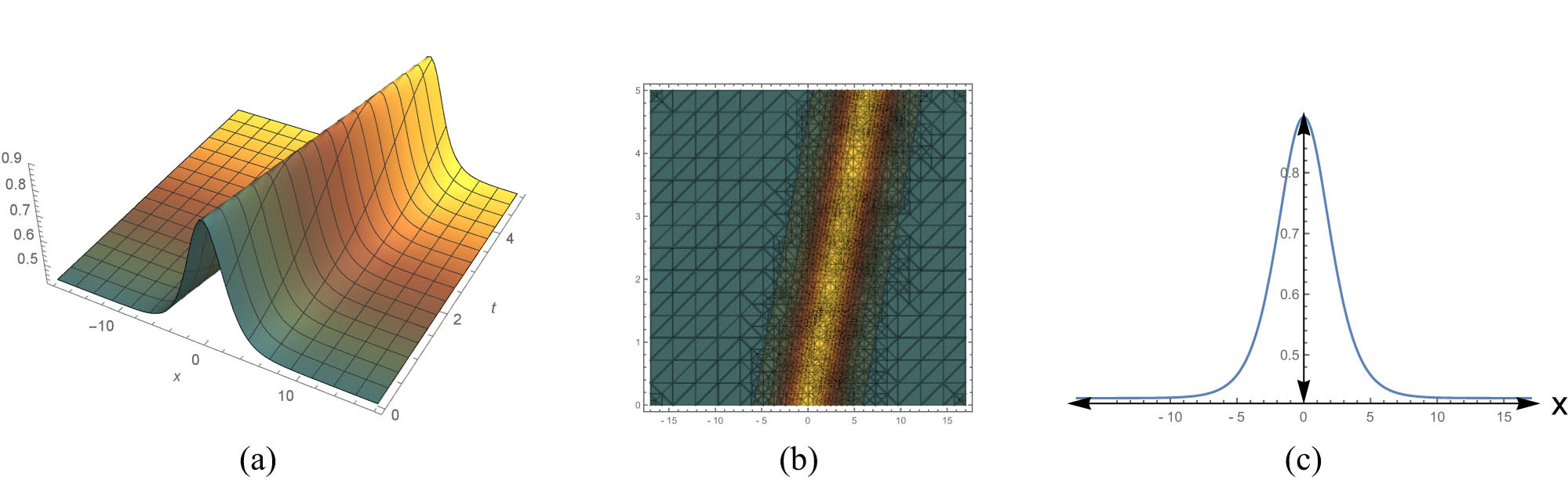
Bright solitary solution of (13): (a) 3D, (b) contour, and (c) 2D.
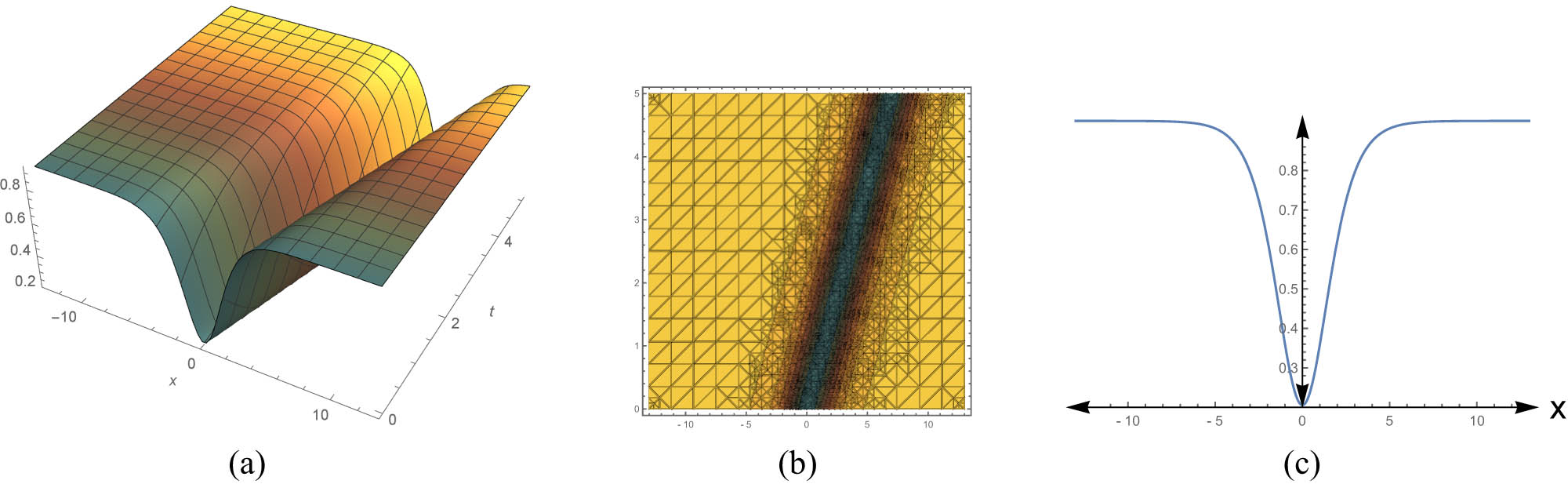
Dark solitary solution (24): (a) 3D, (b) contour, and (c) 2D.
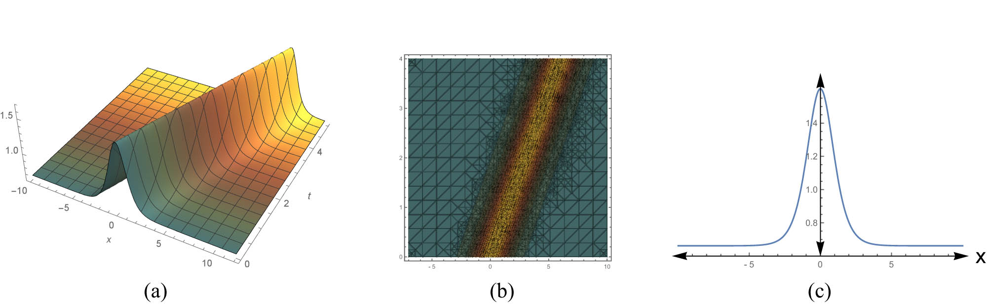
Bright solitary solution of (82): (a) 3D, (b) contour, and (c) 2D.
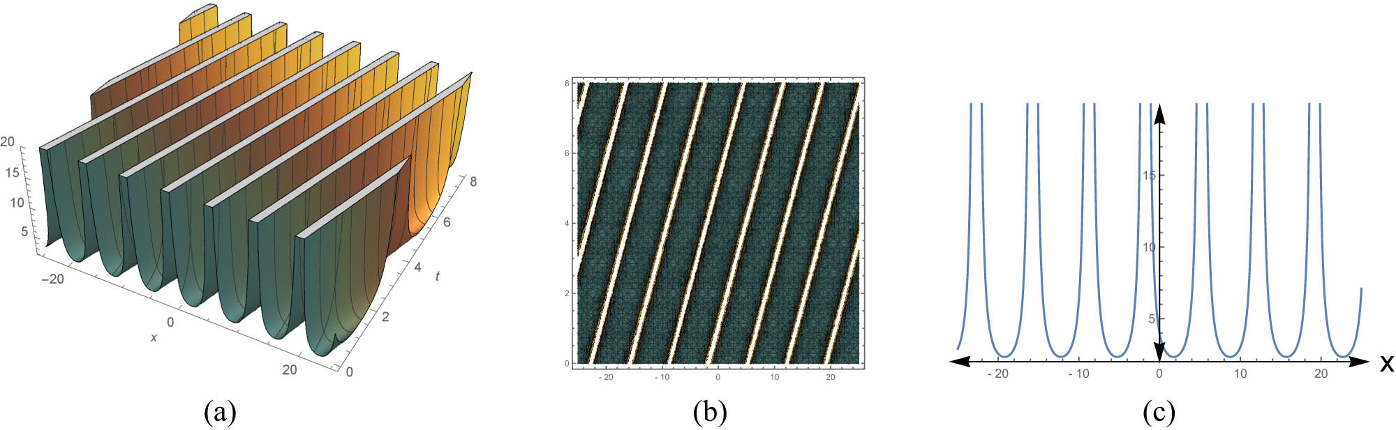
Periodic solution of (96): (a) 3D, (b) contour, and (c) 2D.
6 Results and discussion
The proposed model (7) was studied in the study by Arshad et al. [22] under the constraint
7 Conclusion
In this work, the strain wave model has been studied successfully using the modified extended direct algebraic method. The advantage of the proposed method is that it provides many new exact traveling wave solutions with certain free parameters. Exact solutions are extremely important in interpreting the inner structures of the natural phenomena. The explicit solutions represented several forms of solitary wave solutions based on the variation of the physical parameters. In different articles [6,21–25], only a few traveling wave solutions are extracted to this model that does not provide a complete representation of the physical phenomena. With the aid of the proposed method, novel exact wave solutions are extracted for this model such as bright solitary solutions, dark solitary solutions, singular solitary solutions, singular-dark combo solitary solutions, periodic solutions, Jacobi elliptic function solutions, and other solutions. The extracted solutions confirmed the efficacy and strength of the current technique. Also, this method can be applied to study many other NLPDEs, which frequently arise in engineering, mathematical physics, and other scientific real-time application fields. Moreover, for the physical illustration of the obtained solutions, 2D, contour, and 3D graphs are presented.
In the future, this work may be extended for stochastic strain wave model in micro-structured solids.
-
Funding information: Not available.
-
Author contributions: All authors have accepted responsibility for the entire content of this manuscript and approved its submission.
-
Conflict of interest: The authors have no conflict of interest.
-
Data availability statement: All data are included inside the manuscript.
References
[1] Topsakal M, Taşcan F. Exact traveling wave solutions for space–time-fractional Klein–Gordon equation and (2+1)-Dimensional time-fractional Zoomeron equation via auxiliary equation method. Appl Math Nonlinear Sci. 2020;5(1):437–46. 10.2478/amns.2020.1.00041Search in Google Scholar
[2] Jafari H, Soltani R, Khalique CM, Baleanu D. Exact solutions of two nonlinear partial differential equations by using the first integral method. Boundary Value Problems. 2013 Dec;2013:1–9. 10.1186/1687-2770-2013-117Search in Google Scholar
[3] El-Horbaty MM, Ahmed FM. The solitary traveling wave solutions of some nonlinear partial differential equations using the modified extended tanh function method with Riccati equation. Asian Res J Math. 2018;8(3):1–3. 10.9734/ARJOM/2018/36887Search in Google Scholar
[4] Seadawy AR, Arshad M, Lu D. The weakly nonlinear wave propagation theory for the Kelvin–Helmholtz instability in magnetohydrodynamics flows. Chaos Soliton Fractal. 2020 Oct 1;139:110141. 10.1016/j.chaos.2020.110141Search in Google Scholar
[5] Arshad M, Seadawy AR, Lu D, Saleem MS. Elliptic function solutions, modulation instability and optical solitons analysis of the paraxial wave dynamical model with Kerr media. Optical Quantum Electr. 2021 Jan;53:1–20. 10.1007/s11082-020-02637-6Search in Google Scholar
[6] Arshad M, Seadawy AR, Lu DC, Ali A.Dispersive solitary wave solutions of strain wave dynamical model and its stability. Commun Theoretic Phys. 2019 Oct 1;71(10):1155. 10.1088/0253-6102/71/10/1155Search in Google Scholar
[7] Ali A, Seadawy AR, Lu D. New solitary wave solutions of some nonlinear models and their applications. Adv Differ Equ. 2018 Dec;2018:1–2. 10.1186/s13662-018-1687-7Search in Google Scholar
[8] Lu D, Seadawy R, Ali A. Structure of traveling wave solutions for some nonlinear models via modified mathematical method. Open Phys. 2018 Dec 31;16(1):854–60. 10.1515/phys-2018-0107Search in Google Scholar
[9] Mohyud-Din ST, Irshad A. Solitary wave solutions of some nonlinear PDEs arising in electronics. Optical Quantum Electr. 2017 Apr;49:1–2. 10.1007/s11082-017-0895-9Search in Google Scholar
[10] Seadawy AR, Lu D, Nasreen N. Construction of solitary wave solutions of some nonlinear dynamical system arising in nonlinear water wave models. Indian J Phys. 2020 Nov;94:1785–94. 10.1007/s12648-019-01608-2Search in Google Scholar
[11] Samir I, Badra N, Seadawy AR, Ahmed HM, Arnous AH. Exact wave solutions of the fourth order non-linear partial differential equation of optical fiber pulses by using different methods. Optik. 2021 Mar 1;230:166313. 10.1016/j.ijleo.2021.166313Search in Google Scholar
[12] El-Sheikh MM, Seadawy AR, Ahmed HM, Arnous AH, Rabie WB. Dispersive and propagation of shallow water waves as a higher order nonlinear Boussinesq-like dynamical wave equations. Phys A Stat Mechanics Appl. 2020 Jan 1;537:122. 10.1016/j.physa.2019.122662Search in Google Scholar
[13] Donfack EF, Nguenang JP, Nana L. On the traveling waves in nonlinear electrical transmission lines with intrinsic fractional-order using discrete tanh method. Chaos Solitons Fractals. 2020 Feb 1;131:109486. 10.1016/j.chaos.2019.109486Search in Google Scholar
[14] Park C, Nuruddeen RI, Ali KK, Muhammad L, Osman MS, Baleanu D. Novel hyperbolic and exponential ansatz methods to the fractional fifth-order Korteweg–de Vries equations. Adv Differ Equ. 2020 Dec;2020(1):1–2. 10.1186/s13662-020-03087-wSearch in Google Scholar
[15] Nisar KS, Ilhan OA, Abdulazeez ST, Manafian J, Mohammed SA, Osman MS. Novel multiple soliton solutions for some nonlinear PDEs via multiple Exp-function method. Results Phys. 2021 Feb 1;21:103769. 10.1016/j.rinp.2020.103769Search in Google Scholar
[16] Siddique I, Jaradat MM, Zafar A, Mehdi KB, Osman MS. Exact traveling wave solutions for two prolific conformable M-Fractional differential equations via three diverse approaches. Results Phys. 2021 Sep 1;28:104557. 10.1016/j.rinp.2021.104557Search in Google Scholar
[17] Djennadi S, Shawagfeh N, Osman MS, Gómez-Aguilar JF, Arqub OA. The Tikhonov regularization method for the inverse source problem of time-fractional heat equation in the view of ABC-fractional technique. Phys Scr. 2021 Jun 15;96(9):094006. 10.1088/1402-4896/ac0867Search in Google Scholar
[18] Malik S, Almusawa H, Kumar S, Wazwaz AM, Osman MS. A (2+1)-dimensional Kadomtsev–Petviashvili equation with competing dispersion effect: Painlevé analysis, dynamical behavior and invariant solutions. Results Phys. 2021 Apr 1;23:104043. 10.1016/j.rinp.2021.104043Search in Google Scholar
[19] Liu JG, Osman MS. Nonlinear dynamics for different nonautonomous wave structures solutions of a 3D variable-coefficient generalized shallow water wave equation. Chinese J Phys. 2022 Jun 1;77:1618–24. 10.1016/j.cjph.2021.10.026Search in Google Scholar
[20] Yao SW, Islam ME, Akbar MA, Inc M, Adel M, Osman MS. Analysis of parametric effects in the wave profile of the variant Boussinesq equation through two analytical approaches. Open Phys. 2022 Aug 14;20(1):778–94. 10.1515/phys-2022-0071Search in Google Scholar
[21] Silambarasan R, Baskonus HM, Anand RV, Dinakaran M, Balusamy B, Gao W. Longitudinal strain waves propagating in an infinitely long cylindrical rod composed of generally incompressible materials and its Jacobi elliptic function solutions. Math Comput Simulat. 2021 Apr 1;182:566–602. 10.1016/j.matcom.2020.11.011Search in Google Scholar
[22] Arshad M, Seadawy AR, Lu D. Study of bright-dark solitons of strain wave equation in micro-structured solids and its applications. Modern Phys Lett B. 2019 Nov 30;33(33):1950417. 10.1142/S0217984919504177Search in Google Scholar
[23] Porubov AV, Pastrone F. Non-linear bell-shaped and kink-shaped strain waves in microstructured solids. Int J Non-Linear Mechanics. 2004 Oct 1;39(8):1289–99. 10.1016/j.ijnonlinmec.2003.09.002Search in Google Scholar
[24] Kumar S, Kumar A, Wazwaz AM. New exact solitary wave solutions of the strain wave equation in microstructured solids via the generalized exponential rational function method. Europ Phys J Plus. 2020 Nov;135(11):1–7. 10.1140/epjp/s13360-020-00883-xSearch in Google Scholar
[25] Nofal TA, Samir I, Badra N, Darwish A, Ahmed HM, Arnous AH. Constructing new solitary wave solutions to the strain wave model in micro-structured solids. Alexandria Eng J. 2022 Dec 1;61(12):11879–88. 10.1016/j.aej.2022.05.050Search in Google Scholar
[26] Biswas A. Quasi-stationary non-Kerr law optical solitons. Optical Fiber Technol. 2003 Oct 1;9(4):224–59. 10.1016/S1068-5200(03)00044-0Search in Google Scholar
[27] Mirzazadeh M, Yıldırım Y, Yaşar E, Triki H, Zhou Q, Moshokoa SP, et al. Optical solitons and conservation law of Kundu-Eckhaus equation. Optik. 2018 Feb 1;154:551–7. 10.1016/j.ijleo.2017.10.084Search in Google Scholar
[28] Biswas A. Optical soliton cooling with polynomial law of nonlinear refractive index. J Optics. 2020 Dec;49(4):580–3. 10.1007/s12596-020-00644-0Search in Google Scholar
[29] Seadawy AR, Yaro D, Lu D. Propagation of nonlinear waves with a weak dispersion via coupled (2+1)-dimensional Konopelchenko-Dubrovsky dynamical equation. Pramana. 2020 Dec;94:1–6. 10.1007/s12043-019-1879-zSearch in Google Scholar
[30] Seadawy AR, Arshad M, Lu D. Stability analysis of new exact traveling-wave solutions of new coupled KdV and new coupled Zakharov-Kuznetsov systems. Europ Phys J Plus. 2017 Apr;132:1–9. 10.1140/epjp/i2017-11437-5Search in Google Scholar
[31] Lu D, Seadawy AR, Arshad M, Wang J. New solitary wave solutions of (3+1)-dimensional nonlinear extended Zakharov-Kuznetsov and modified KdV-Zakharov-Kuznetsov equations and their applications. Results Phys. 2017 Jan 1;7:899–909. 10.1016/j.rinp.2017.02.002Search in Google Scholar
[32] Taghizadeh N, Foumani MN. Using a reliable method for higher dimensional of the fractional Schrödinger equation. Punjab Univ J Math. 2020 Nov 20;48(1). Search in Google Scholar
[33] Samsonov AM. Strain solitons in solids and how to construct them. Boca Raton: CRC Press; 2001. p. 1–229.10.1201/9781420026139Search in Google Scholar
© 2024 the author(s), published by De Gruyter
This work is licensed under the Creative Commons Attribution 4.0 International License.
Articles in the same Issue
- Editorial
- Focus on NLENG 2023 Volume 12 Issue 1
- Research Articles
- Seismic vulnerability signal analysis of low tower cable-stayed bridges method based on convolutional attention network
- Robust passivity-based nonlinear controller design for bilateral teleoperation system under variable time delay and variable load disturbance
- A physically consistent AI-based SPH emulator for computational fluid dynamics
- Asymmetrical novel hyperchaotic system with two exponential functions and an application to image encryption
- A novel framework for effective structural vulnerability assessment of tubular structures using machine learning algorithms (GA and ANN) for hybrid simulations
- Flow and irreversible mechanism of pure and hybridized non-Newtonian nanofluids through elastic surfaces with melting effects
- Stability analysis of the corruption dynamics under fractional-order interventions
- Solutions of certain initial-boundary value problems via a new extended Laplace transform
- Numerical solution of two-dimensional fractional differential equations using Laplace transform with residual power series method
- Fractional-order lead networks to avoid limit cycle in control loops with dead zone and plant servo system
- Modeling anomalous transport in fractal porous media: A study of fractional diffusion PDEs using numerical method
- Analysis of nonlinear dynamics of RC slabs under blast loads: A hybrid machine learning approach
- On theoretical and numerical analysis of fractal--fractional non-linear hybrid differential equations
- Traveling wave solutions, numerical solutions, and stability analysis of the (2+1) conformal time-fractional generalized q-deformed sinh-Gordon equation
- Influence of damage on large displacement buckling analysis of beams
- Approximate numerical procedures for the Navier–Stokes system through the generalized method of lines
- Mathematical analysis of a combustible viscoelastic material in a cylindrical channel taking into account induced electric field: A spectral approach
- A new operational matrix method to solve nonlinear fractional differential equations
- New solutions for the generalized q-deformed wave equation with q-translation symmetry
- Optimize the corrosion behaviour and mechanical properties of AISI 316 stainless steel under heat treatment and previous cold working
- Soliton dynamics of the KdV–mKdV equation using three distinct exact methods in nonlinear phenomena
- Investigation of the lubrication performance of a marine diesel engine crankshaft using a thermo-electrohydrodynamic model
- Modeling credit risk with mixed fractional Brownian motion: An application to barrier options
- Method of feature extraction of abnormal communication signal in network based on nonlinear technology
- An innovative binocular vision-based method for displacement measurement in membrane structures
- An analysis of exponential kernel fractional difference operator for delta positivity
- Novel analytic solutions of strain wave model in micro-structured solids
- Conditions for the existence of soliton solutions: An analysis of coefficients in the generalized Wu–Zhang system and generalized Sawada–Kotera model
- Scale-3 Haar wavelet-based method of fractal-fractional differential equations with power law kernel and exponential decay kernel
- Non-linear influences of track dynamic irregularities on vertical levelling loss of heavy-haul railway track geometry under cyclic loadings
- Fast analysis approach for instability problems of thin shells utilizing ANNs and a Bayesian regularization back-propagation algorithm
- Validity and error analysis of calculating matrix exponential function and vector product
- Optimizing execution time and cost while scheduling scientific workflow in edge data center with fault tolerance awareness
- Estimating the dynamics of the drinking epidemic model with control interventions: A sensitivity analysis
- Online and offline physical education quality assessment based on mobile edge computing
- Discovering optical solutions to a nonlinear Schrödinger equation and its bifurcation and chaos analysis
- New convolved Fibonacci collocation procedure for the Fitzhugh–Nagumo non-linear equation
- Study of weakly nonlinear double-diffusive magneto-convection with throughflow under concentration modulation
- Variable sampling time discrete sliding mode control for a flapping wing micro air vehicle using flapping frequency as the control input
- Error analysis of arbitrarily high-order stepping schemes for fractional integro-differential equations with weakly singular kernels
- Solitary and periodic pattern solutions for time-fractional generalized nonlinear Schrödinger equation
- An unconditionally stable numerical scheme for solving nonlinear Fisher equation
- Effect of modulated boundary on heat and mass transport of Walter-B viscoelastic fluid saturated in porous medium
- Analysis of heat mass transfer in a squeezed Carreau nanofluid flow due to a sensor surface with variable thermal conductivity
- Navigating waves: Advancing ocean dynamics through the nonlinear Schrödinger equation
- Experimental and numerical investigations into torsional-flexural behaviours of railway composite sleepers and bearers
- Novel dynamics of the fractional KFG equation through the unified and unified solver schemes with stability and multistability analysis
- Analysis of the magnetohydrodynamic effects on non-Newtonian fluid flow in an inclined non-uniform channel under long-wavelength, low-Reynolds number conditions
- Convergence analysis of non-matching finite elements for a linear monotone additive Schwarz scheme for semi-linear elliptic problems
- Global well-posedness and exponential decay estimates for semilinear Newell–Whitehead–Segel equation
- Petrov-Galerkin method for small deflections in fourth-order beam equations in civil engineering
- Solution of third-order nonlinear integro-differential equations with parallel computing for intelligent IoT and wireless networks using the Haar wavelet method
- Mathematical modeling and computational analysis of hepatitis B virus transmission using the higher-order Galerkin scheme
- Mathematical model based on nonlinear differential equations and its control algorithm
- Bifurcation and chaos: Unraveling soliton solutions in a couple fractional-order nonlinear evolution equation
- Space–time variable-order carbon nanotube model using modified Atangana–Baleanu–Caputo derivative
- Minimal universal laser network model: Synchronization, extreme events, and multistability
- Valuation of forward start option with mean reverting stock model for uncertain markets
- Geometric nonlinear analysis based on the generalized displacement control method and orthogonal iteration
- Fuzzy neural network with backpropagation for fuzzy quadratic programming problems and portfolio optimization problems
- B-spline curve theory: An overview and applications in real life
- Nonlinearity modeling for online estimation of industrial cooling fan speed subject to model uncertainties and state-dependent measurement noise
- Quantitative analysis and modeling of ride sharing behavior based on internet of vehicles
- Review Article
- Bond performance of recycled coarse aggregate concrete with rebar under freeze–thaw environment: A review
- Retraction
- Retraction of “Convolutional neural network for UAV image processing and navigation in tree plantations based on deep learning”
- Special Issue: Dynamic Engineering and Control Methods for the Nonlinear Systems - Part II
- Improved nonlinear model predictive control with inequality constraints using particle filtering for nonlinear and highly coupled dynamical systems
- Anti-control of Hopf bifurcation for a chaotic system
- Special Issue: Decision and Control in Nonlinear Systems - Part I
- Addressing target loss and actuator saturation in visual servoing of multirotors: A nonrecursive augmented dynamics control approach
- Collaborative control of multi-manipulator systems in intelligent manufacturing based on event-triggered and adaptive strategy
- Greenhouse monitoring system integrating NB-IOT technology and a cloud service framework
- Special Issue: Unleashing the Power of AI and ML in Dynamical System Research
- Computational analysis of the Covid-19 model using the continuous Galerkin–Petrov scheme
- Special Issue: Nonlinear Analysis and Design of Communication Networks for IoT Applications - Part I
- Research on the role of multi-sensor system information fusion in improving hardware control accuracy of intelligent system
- Advanced integration of IoT and AI algorithms for comprehensive smart meter data analysis in smart grids