Optimize the corrosion behaviour and mechanical properties of AISI 316 stainless steel under heat treatment and previous cold working
-
Haider Mahdi Lieth
 ,
Basil Sh. Munahi
,
Basil Sh. Munahi

Abstract
Improving corrosion resistance in alloys made of stainless steel is an important innovation on the petroleum trade. The effect of heat treatments (HT) and cold working on the corrosion behaviour, surface hardness, and microstructure of 316 stainless steel was investigated experimentally. The corrosion environment is seawater and crude oil. The corrosion rates (CRs) were obtained using the mean loss of weight approach, which was then optimised using the Taguchi method. The specimens used in this study are made of 316 stainless steel rod, which is first annealed to obtain the qualities of the raw material before being put through a tensile test to assess the mechanical characteristics of the metal. After cold working, the hardness test, the corrosion test utilising the lost weight method, and the microstructure test are all carried out. By performing these tests, the metal show excellent mechanical properties such as yield stress, tensile stress, and hardness; in the corrosion test, the raw metal show higher resistance in both seawater and crude oil, while in cold working and HT with cold working, samples show higher corrosion The HT samples had the lowest corrosion resistance as the cold working percentage increased. In this work, the input parameters such as ultimate corrosion media, HT and cold work (CW) are optimised utilising a multiple objective optimisation approach that uses weighted grey relational analysis. Two objectives, that are CR and Hardness (H), are simultaneously optimised. We suggested a quantitative approach to establish the weight factors of various responses for grey relational analysis called weighted grey relational analysis. The optimum input parameters were determined using weighted grey relational analysis, and the outcomes showed that HT is the most relevant parameter. Cold working has been observed in association with stress-related twinning and austenite phase deformation, resulting in fast grain splitting and the production of a microstructure that resembles a ribbon composed of austenite and ferrite.
1 Introduction
Austenitic stainless steels (SS) are commonly used in many instances of industrial and construction industries due to their passivation feature and ability to tolerate environmental deterioration. Their outstanding mechanical performance and corrosion resistance at both high and low temperatures are largely responsible for this wide range of applications. However, intergranular corrosion poses a serious threat to them [1,2,3]. The majority of biomedical applications for austenitic stainless steels include implants, fittings, medicines, and surgical instruments. The biocompatibility, low cost, ease of manufacture, exceptionally high mechanical strength, and resistance to corrosion of 316L stainless steel contribute to its widespread application [4,5,6].
Heat treatment (HT) cannot harden 316 stainless steel. Rapid cooling can be used to perform annealing or solution treatment after heating to 1,010–1,120°C [7].
Rather than being heated, such stainless steel can be toughened by cold working. Intergranular corrosion can result from heat treating stainless steel as well as chromium and C depletion at grain boundaries [8]. However, by limiting the diffusion channel for carbon together with chromium in the fine granules, stainless steel grain refinement could significantly enhance corrosion resistance. Because of this, there is less chance of chromium depletion at grain boundaries, which would encourage the development of an identical passive oxide coating on the surface and prevent 316L stainless steel from dissolving [8,9,10].
The 316L steel has a very low strength. HTs cannot strengthen these steels since they do not go through any phase transformations. However, they may be made stronger by reducing the grain size to submicrometer levels [11,12].
Plastic deformation has the ability to alter the characteristics of a material by increasing the dislocation density, decreasing the percentage of coincidence site lattice barriers, introducing deformation bands, and even changing the phase [13,14]. The corrosion and cracking resistance of austenitic stainless steels in settings would be impacted by these modifications to the material and mechanical characteristics. Austenitic stainless steel achieves a passive state with high stability and strong corrosion resistance when chromium is present in some quantity [15,16]. It has been found that increasing the quantity of cold-working produced tensile and yield strength improvements for austenitic stainless steels. This can be done as a percentage, such as 10, 20%, and so on [17,18,19].
316 austenitic stainless steel has been the subject of several studies on corrosion rates (CRs); however, there has been little study on how pre-cold working and annealing temperature affect 316 CRs. These impacts at various levels and in diverse corrosive settings are made clear by the current investigation. In addition, each environment’s mechanical properties and microstructure were examined, and the most efficient elements of the process were investigated.
2 Experimental work
2.1 Raw materials and HT
Three 316 stainless steel rods were selected, each measuring 1.87 m in length and 10 mm in diameter. As indicated in Table 1, a PECTROTEST TXC25 spectrometer was utilised to ascertain the chemical composition for a double check.
Lists the chemical constitution of 316 stainless steel in percentages
| Fe | C | Si | Mn | Cr | Ni | Cu | P | S | Co | |
|---|---|---|---|---|---|---|---|---|---|---|
| Measured | Bal. | 0.037 | 0.215 | 1.19 | 17.13 | 11.89 | 0.45 | 0.0187 | 0.012 | 0.154 |
| Maximum (%) | Bal. | 0.07 | 1 | 2 | 18.5 | 13 | 0.045 | 0.03 |
According to the ultimate corrosion media (CM), either saltwater or crude oil, the samples were split into two primary groups, each of which was further separated into three parts (without HT, annealing at 1,160°C and quenching with water, and annealing at 1,160°C and quenching with oil). Three parts of each specimen group are divided into three smaller groups, each of which is subjected to 10, 20, and 30% cold working, respectively, according to ASTM E8M [19] utilising a universal tensile machine. Each group from 20 groups contains three specimens according to the cold working and immersion media environments as shown in Table 2.
Specimen classification based on cold working and immersion media
| Group | HT | Cold working | Quenching media | Ultimate CM |
|---|---|---|---|---|
| 1 | Without | Without | Without | Crude oil |
| 2 | Without | Without | Without | Seawater |
| 3 | Without | 10% | Without | Seawater |
| 4 | Without | 20% | Without | Seawater |
| 5 | Without | 30% | Without | Seawater |
| 6 | Without | 10% | Without | Crude oil |
| 7 | Without | 20% | Without | Crude oil |
| 8 | Without | 30% | Without | Crude oil |
| 9 | Annealing at 1,160°C | 10% | Oil | Crude oil |
| 10 | Annealing at 1,160°C | 20% | Oil | Crude oil |
| 11 | Annealing at 1,160°C | 30% | Oil | Crude oil |
| 12 | Annealing at 1,160°C | 10% | Oil | Seawater |
| 13 | Annealing at 1,160°C | 20% | Oil | Seawater |
| 14 | Annealing at 1,160°C | 30% | Oil | Seawater |
| 15 | Annealing at 1,160°C | 10% | Water | Seawater |
| 16 | Annealing at 1,160°C | 20% | Water | Seawater |
| 17 | Annealing at 1,160°C | 30% | Water | Seawater |
| 18 | Annealing at 1,160°C | 10% | Water | Crude oil |
| 19 | Annealing at 1,160°C | 20% | Water | Crude oil |
| 20 | Annealing at 1,160°C | 30% | Water | Crude oil |
The hardness test was performed in accordance with ASTM E384 [20]. After machining the metal as shown in Figure 1, in the first two cases, the specimens were kept unprocessed simply by being placed in seawater and crude oil, while the other examples were subjected to 10, 20, and 30% cold working, respectively, and annealing. The process of annealing was used to create 316 stainless steel. After being submerged at 1,160°C, Type 316 is quenched in either water or air.

Tension test specimen.
2.2 Aggressive environments
The impact of annealing and pre-cold on the corrosion resistance of the 316 stainless steel was examined using two corrosive media. The corrosive environment consists of seawater and crude oil. Table 3 lists the characteristics of seawater, while Table 4 lists the characteristics of the crude oil utilised in the experiment.
Properties of sea water
| Test | Seawater |
|---|---|
| Temperature (°C) | 16 |
| Mass density (kg/m3) | 1027.03 |
| Kinematic viscosity (m2/s) | 1.1978 × 10⁻⁶ |
| PH | 8.12 |
| Dynamic viscosity (Pa s) | 0.001324 |
Crude oil’s characteristics
| Test | Results | Method |
|---|---|---|
| Density (g/cm3) at 15°C | 0.95 | ASTM D-1298 |
| Flash point (°C) | 139.00 | ASTM D-93 |
| Kinematic viscosity (m2/s) | 371.20 | ASTM D-445 |
| Pour point (°C) | −3.00 | ASTM D-97 |
| Sulphur contact (wt%) | 4.53 | ASTM D-4294 |
| Carbon residue (RAMS) (wt%) | 9.54 | ASTM D-524 |
| Water and sediment (vol%) | 0.11 | ASTM D-1796 |
The majority of the oil produced in Iraq is exported via the Arabian Gulf; therefore, sea water measurements from the Arabian Gulf must be taken. This is because there are numerous export platforms (including Khor al-Zubayr in the Basra Governorate and the port of Umm Qasr).
2.3 Corrosion test
The corrosion of the samples was examined using the loss-weight method in conformity with ASTM G31 [21], a standard. The specimens were cleaned correctly, with the use of chemical and mechanical cleaners to eliminate any contaminants and any oxidisation layer (if present). To avoid the inaccurate and deceptive findings of short-period tests, a certain container was used, and the appropriate test period was picked. The tests were set up as cases submerged in settings including seawater and crude oil. The container was shut tightly and kept for a week. To determine the weight lost, the specimens were taken out and cleaned every week. The CR was calculated using the following equation [22]:
where ρ is the metal density in grams per cubic centimetre, A is the specimen’s area in square centimetres (cm2), t is the exposure duration in hours, m is weight loss in milligrams, and CR is the CR in millimetres per year (MPY). In Table 5, a portion of the weight loss calculations is shown.
Weight loss for sea water samples
| Sample | Week zero | Week 1 | Week 2 | Week 3 | Week 4 | Weight loos week 1 | Weight loos week 2 | Weight loos week 3 | Weight loos week 4 |
|---|---|---|---|---|---|---|---|---|---|
| Shaft without | 12.2625 | 12.2618 | 12.2613 | 12.261 | 12.2608 | 0.0007 | 0.0012 | 0.0015 | 0.0017 |
| Without HT 10% | 12.4981 | 12.4979 | 12.4977 | 12.4975 | 12.4973 | 0.0002 | 0.0004 | 0.0006 | 0.0008 |
| Without HT 20% | 12.4482 | 12.448 | 12.4479 | 12.4477 | 12.4476 | 0.0002 | 0.0003 | 0.0005 | 0.0006 |
| Without HT 30% | 12.5585 | 12.558 | 12.5577 | 12.557 | 12.5549 | 0.0005 | 0.0008 | 0.0015 | 0.0036 |
| 1,160°C → cooling in oil 10% | 12.6498 | 12.6492 | 12.6476 | 12.6449 | 12.6411 | 0.0006 | 0.0022 | 0.0049 | 0.0087 |
| 1,160°C → cooling in oil 20% | 12.615 | 12.6131 | 12.6122 | 12.6118 | 12.6113 | 0.0019 | 0.0028 | 0.0032 | 0.0037 |
| 1,160°C → cooling in oil 30% | 12.2255 | 12.2252 | 12.2232 | 12.222 | 12.2214 | 0.0003 | 0.0023 | 0.0035 | 0.0041 |
| 1,160°C → cooling in water 10% | 12.5063 | 12.5045 | 12.5043 | 12.5031 | 12.5022 | 0.0018 | 0.002 | 0.0032 | 0.0041 |
| 1,160°C → cooling in water 20% | 12.4495 | 12.449 | 12.4478 | 12.4471 | 12.4466 | 0.0005 | 0.0017 | 0.0024 | 0.0029 |
| 1,160°C → cooling in water 30% | 12.5789 | 12.5771 | 12.5767 | 12.5729 | 12.5721 | 0.0018 | 0.0022 | 0.006 | 0.0068 |
2.4 Analysis and design of experimental data
The total number of the input parameters, their involvement in research, as well as their levels, influence the design of experiments (DOE) that will be utilised to perform the experiments. The L20 array is created in the current experiment using the Taguchi approach, and subsequent processing is progressed correspondingly. Furthermore, the strength of the chosen design is guaranteed. A powerful design is one that noise or other uncontrolled events have the least impact possible on the response variables. The next sections provide specifics on the experiment and analytic method utilised in the current study for multi-response optimisation.
2.4.1 Optimisation parameters
The input parameters used in the current analysis are ultimate CM, HT, and cold work (CW). The parameters, units, and levels as indicated in Table 6.
Parameters of input and their levels
| Input parameters | Symbol | Unit | Level 1 | Level 2 | Level 3 | Level 4 |
|---|---|---|---|---|---|---|
| Ultimate CM | CM | Sea Water CM1 | Crude Oil CM2 | |||
| HT | HT | without HT1 | Annealing at 1,160°C | Annealing at 1,160°C | ||
| Quenching in oil | Quenching in water | |||||
| HT2 | HT3 | |||||
| Cold work | CW | 0 | 10 | 20 | 30 |
2.4.2 Response variables
CR and hardness (H) were examined as two response variables. CR minimisation and Hardness (H) maximisation were the goals. Table 7 displays the response variables along with the abbreviations and units.
Response variables
| No | Response variables | Abbreviation | Unit |
|---|---|---|---|
| 1 | CR | CR | mpy |
| 2 | Hardness | H | N/mm² |
2.4.3 Experimental data array
With fewer experiments, the experimental data array may be used to examine how a system’s or process’s input parameters impact the response variables. The Taguchi technique is used to do this. The number of input parameters utilised in the experiment, together with their levels, determine the experimental data array. The L20 data array was used for the current investigation, as indicated in Table 8. The data analysis may be carried out using a standard statistical programme like Minitab; in the current study, the tool used for this was Minitab18.
Experimental data array
| Exp. No | CM | HT | CW | Exp. No | CM | HT | CW |
|---|---|---|---|---|---|---|---|
| 1 | CM1 | HT1 | 0 | 11 | CM2 | HT1 | 0 |
| 2 | CM1 | HT1 | 10 | 12 | CM2 | HT1 | 10 |
| 3 | CM1 | HT1 | 20 | 13 | CM2 | HT1 | 20 |
| 4 | CM1 | HT1 | 30 | 14 | CM2 | HT1 | 30 |
| 5 | CM1 | HT2 | 10 | 15 | CM2 | HT2 | 10 |
| 6 | CM1 | HT2 | 20 | 16 | CM2 | HT2 | 20 |
| 7 | CM1 | HT2 | 30 | 17 | CM2 | HT2 | 30 |
| 8 | CM1 | HT3 | 10 | 18 | CM2 | HT3 | 10 |
| 9 | CM1 | HT3 | 20 | 19 | CM2 | HT3 | 20 |
| 10 | CM1 | HT3 | 30 | 20 | CM2 | HT3 | 30 |
2.4.4 Signal-to-noise ratio calculation and analysis
The signal-to-noise (S/N) ratio for each factor level combination is calculated. Since the goal was to reduce the CR, the smaller-is-better criteria was applied, and Eq. (2) is utilised to obtain the S/N ratio. Similarly, as the goal was to maximise hardness (H), the larger-is-better criteria was applied, and the S/N ratio is determined using Eq. (3).
The following is the S/N ratio for the smaller-the-better characteristic:
The S/N ratio for the larger-the-better feature is also written as follows:
where y i stands for the observed response values for each run, and n stands for the experimental sets. Table 9 shows the S/N ratio for CR and H depending on Eqs. (2) and (3).
S/N ratio for CR and H with their calculated values
| Exp. No | CM | HT | CW | CR | H | CR S/N ratio | H S/N ratio |
|---|---|---|---|---|---|---|---|
| 1 | CM1 | HT1 | 0 | 0.143876781 | 184 | 16.8402 | 45.2964 |
| 2 | CM1 | HT1 | 10 | 0.066716407 | 198.5 | 23.5153 | 45.9552 |
| 3 | CM1 | HT1 | 20 | 0.050352548 | 203 | 25.9596 | 46.1499 |
| 4 | CM1 | HT1 | 30 | 0.300293095 | 229 | 10.4491 | 47.1967 |
| 5 | CM1 | HT2 | 10 | 0.71948974 | 96 | 2.8595 | 39.6454 |
| 6 | CM1 | HT2 | 20 | 0.306930175 | 103 | 10.2592 | 40.2567 |
| 7 | CM1 | HT2 | 30 | 0.345052859 | 94 | 9.2423 | 39.4626 |
| 8 | CM1 | HT3 | 10 | 0.345731672 | 100 | 9.2252 | 40.0000 |
| 9 | CM1 | HT3 | 20 | 0.242799663 | 127 | 12.2950 | 42.0761 |
| 10 | CM1 | HT3 | 30 | 0.582217968 | 90 | 4.6983 | 39.0849 |
| 11 | CM2 | HT1 | 0 | 0.138065687 | 152 | 17.1983 | 43.6369 |
| 12 | CM2 | HT1 | 10 | 0.051667957 | 200 | 25.7356 | 46.0206 |
| 13 | CM2 | HT1 | 20 | 0.135684539 | 221 | 17.3494 | 46.8878 |
| 14 | CM2 | HT1 | 30 | 0.070028183 | 231 | 23.0945 | 47.2722 |
| 15 | CM2 | HT2 | 10 | 0.141415624 | 94 | 16.9901 | 39.4626 |
| 16 | CM2 | HT2 | 20 | 0.049263307 | 127 | 26.1495 | 42.0761 |
| 17 | CM2 | HT2 | 30 | 0.36404637 | 111 | 8.7769 | 40.9065 |
| 18 | CM2 | HT3 | 10 | 0.17342484 | 103 | 15.2178 | 40.2567 |
| 19 | CM2 | HT3 | 20 | 0.28751917 | 120 | 10.8267 | 41.5836 |
| 20 | CM2 | HT3 | 30 | 0.126789336 | 110 | 17.9383 | 40.8279 |
2.4.5 Grey-Taguchi optimisation technique
We have used a multi-objective optimisation approach since two response parameters are thought to be optimised concurrently. In the current experimental study, we are using grey and Taguchi to optimise the process parameters, and depending on their grade, Taguchi approach is then used to optimise them.
2.4.6 Grey relational technique
Grey relational methodology is a technique for combining many quality factors into one, allowing for the implementation of Taguchi single objective optimisation techniques and multi-objective quality parameter conversions. To do this, grey relational analysis (GRA) is used to determine the grey relational grade (GRG). Less data and multifactor analysis are its defining qualities, and these two traits might outweigh the drawbacks of statistical regression analysis. This single goal optimisation strategy makes advantage of the performance feature known as GRG. A step-by-step description of the GRA process and its outcome is presented [22,23].
2.4.6.1 GRA methodology
The following stages are the order in which GRA is conducted.
2.4.6.1.1 Normalising the S/N ratios
The study’s initial data, which is used to convert the original sequence into an identical sequence, is prepared by normalising the S/N ratio in Taguchi-based GRA. The information in the 0–1 range of values, often known as the “grey relational generation,” are transformed by normalising the S/N ratio. In this study, the smaller the better criterion for CR and the larger the better criterion for normalisation of Hardness (H) are employed, respectively, utilising the equations found in Eqs. (4) and (5) [23].
Smaller the better:
Larger the better:
where max z i (p) is the largest value of z i (p) for the pth respond, min z i (p) is the lowest value of the S/N ratio, u i (p) is the outcome of grey relational generation. The normalised data are presented in Table 10.
S/N ratio normalised value for CR and H
| No. | CR | H | No. | CR | H |
|---|---|---|---|---|---|
| u i (p) | u i (p) | u i (p) | u i (p) | ||
| 1 | 0.399713812 | 0.758667502 | 11 | 0.384338166 | 0.55597961 |
| 2 | 0.113103449 | 0.839139277 | 12 | 0.0177739 | 0.847125913 |
| 3 | 0.008156188 | 0.862921038 | 13 | 0.377850071 | 0.953050465 |
| 4 | 0.674127162 | 0.990774843 | 14 | 0.131171455 | 1 |
| 5 | 1 | 0.068468036 | 15 | 0.393279023 | 0.046132762 |
| 6 | 0.682280218 | 0.143134062 | 16 | 0 | 0.365345299 |
| 7 | 0.72594359 | 0.046132762 | 17 | 0.74592732 | 0.222489648 |
| 8 | 0.726676553 | 0.111775533 | 18 | 0.469375053 | 0.143134062 |
| 9 | 0.594868095 | 0.365345299 | 19 | 0.657915463 | 0.305197983 |
| 10 | 0.921048588 | 0 | 20 | 0.352562299 | 0.212888801 |
2.4.6.1.2 Determining the deviation sequence
The difference between the reference sequence y o (p) and the comparability sequence y i (p), following normalisation, is represented by the deviation sequence ∆ oi [23]. Eq. (6) is used to determine it as follows:
The deviation sequence is presented in Table 11.
Deviation sequence for CR and H
| No. | CR | H | No. | CR | H |
|---|---|---|---|---|---|
| Δ oi | Δ oi | Δ oi | Δ oi | ||
| 1 | 0.600286188 | 0.241332498 | 11 | 0.615661834 | 0.44402039 |
| 2 | 0.886896551 | 0.160860723 | 12 | 0.9822261 | 0.152874087 |
| 3 | 0.991843812 | 0.137078962 | 13 | 0.622149929 | 0.046949535 |
| 4 | 0.325872838 | 0.009225157 | 14 | 0.868828545 | 0 |
| 5 | 0 | 0.931531964 | 15 | 0.606720977 | 0.953867238 |
| 6 | 0.317719782 | 0.856865938 | 16 | 1 | 0.634654701 |
| 7 | 0.27405641 | 0.953867238 | 17 | 0.25407268 | 0.777510352 |
| 8 | 0.273323447 | 0.888224467 | 18 | 0.530624947 | 0.856865938 |
| 9 | 0.405131905 | 0.634654701 | 19 | 0.342084537 | 0.694802017 |
| 10 | 0.078951412 | 1 | 20 | 0.647437701 | 0.787111199 |
2.4.6.1.3 Grey relational coefficient
The grey relational coefficient (GRC) is a measure of the connection between the ideal (optimal) and actual normalised S/N ratio for all sequences. The two sequences have a grey relational coefficient of 1 if they agree at every points [23,24]. Eq. (7) may be used to represent the grey relational coefficient GRC.
where
GRC for CR and H
| No. | CR | H | No. | CR | H |
|---|---|---|---|---|---|
| GRC | GRC | GRC | GRC | ||
| 1 | 0.454427226 | 0.674461192 | 11 | 0.448164475 | 0.529649577 |
| 2 | 0.360517156 | 0.756589071 | 12 | 0.337330452 | 0.765844455 |
| 3 | 0.335155729 | 0.78483207 | 13 | 0.445573258 | 0.914161121 |
| 4 | 0.60542008 | 0.981883934 | 14 | 0.365275842 | 1 |
| 5 | 1 | 0.349276169 | 15 | 0.451785057 | 0.343910356 |
| 6 | 0.611456407 | 0.368496243 | 16 | 0.333333333 | 0.440662696 |
| 7 | 0.645947755 | 0.343910356 | 17 | 0.663066059 | 0.391386261 |
| 8 | 0.64655999 | 0.3601723 | 18 | 0.485142536 | 0.368496243 |
| 9 | 0.552405674 | 0.440662696 | 19 | 0.593764614 | 0.418479374 |
| 10 | 0.863630332 | 0.333333333 | 20 | 0.435753505 | 0.388466824 |
Mean value for the CR parameter at each level
| CR | |||
|---|---|---|---|
| Level | CM | HT | CW |
| 1 | 0.607552035 | 0.418983027 | 0.45129585 |
| 2 | 0.455918913 | 0.617598102 | 0.546889198 |
| 3 | 0.596209442 | 0.478614836 | |
| 4 | 0.596515596 | ||
| max | 0.607552035 | 0.617598102 | 0.596515596 |
| min | 0.455918913 | 0.418983027 | 0.45129585 |
| Range = max–min | 0.151633122 | 0.198615075 | 0.145219745 |
| Sum | 0.495467942 | ||
Mean value for the H parameter at each level
| H | |||
|---|---|---|---|
| Level | CM | HT | CW |
| 1 | 0.539361736 | 0.800927677 | 0.602055384 |
| 2 | 0.556105691 | 0.372940347 | 0.490714766 |
| 3 | 0.384935128 | 0.5612157 | |
| 4 | 0.573163451 | ||
| max | 0.556105691 | 0.800927677 | 0.602055384 |
| min | 0.539361736 | 0.372940347 | 0.490714766 |
| Range = max–min | 0.016743954 | 0.42798733 | 0.111340618 |
| Sum | 0.556071903 | ||
2.4.6.1.4 Weight factor calculations
For an actual engineering challenge, different approaches have varying degrees of relevance. The GRG varies significantly when different responses have differing weights, indicating that weight considerations are crucial for attaining the best outcomes. In most cases, researchers employ equal weight to calculate the GRG of numerous replies [25,26] or use a weight to subjectively emphasise or de-emphasize the aim. To provide acceptable values to various responses under optimisation, a sensible criterion for weight factor computation can be utilised [27]. To estimate the weight factors, this technique depends on how much the alterations in the parameters have an impact on the responds. Using Eqs. (8) and (9) correspondingly, the grey relational coefficient ranges and weight factors are calculated. The weighting variables for each response are also shown in the last row of Table 15.
j = 1,2…, p, i = 1,2…, m, and k = 1,2…, l. w, weights, m, responses, p, parameters, l, experimental levels, R, ranges of grey relational coefficients, K, average grey relational coefficients for each parameter at each level of each response, and m, responses. There are specified weighting parameters for the responses, and the calculation for the GRG is provided by
Grey relational coefficients weighing factors
| CR | H | |
|---|---|---|
| Sum | 0.495467942 | 0.556071903 |
| Total sum | 1.051539845 | |
| Weight | 0.471183231 | 0.528816769 |
where GRCCR stands for the grey relational coefficient of CR and GRCH is that for the hardness. Table 16 lists the values for two responses grey relationship grades.
Grey relational grade and rank
| No. | GRG | Rank | No. | GRG | Rank |
|---|---|---|---|---|---|
| 1 | 0.570784877 | 7 | 11 | 0.491255163 | 14 |
| 2 | 0.569966626 | 8 | 12 | 0.563935843 | 9 |
| 3 | 0.572952118 | 6 | 13 | 0.693370378 | 3 |
| 4 | 0.804500479 | 1 | 14 | 0.700928621 | 2 |
| 5 | 0.655886326 | 4 | 15 | 0.394739106 | 19 |
| 6 | 0.482974998 | 16 | 16 | 0.3900909 | 20 |
| 7 | 0.486225314 | 15 | 17 | 0.519397226 | 10 |
| 8 | 0.495113377 | 12 | 18 | 0.42345802 | 17 |
| 9 | 0.493314114 | 13 | 19 | 0.50107084 | 11 |
| 10 | 0.583200387 | 5 | 20 | 0.410747515 | 18 |
2.4.6.1.5 GRG and rank determination
The GRG provides the foundation for the overall assessment of the many performance aspects. The highest rank is given to the grade with the highest value. The computation of the GRG, which acts as a basis for the overall assessment of the multiple-performance feature, is the next stage of GRA and is performed using Eq. (11) [23,28]:
where w p is the weighted factor for each grey relational coefficient and n is the total number of response variables. For each of the response variables, the total weighting factors should equal 1.
3 Results and discussion
3.1 Microhardness
Results for the microhardness of the 316 austenitic stainless steels as received and after HT and cold working are shown in Figure 2 for the groups in Table 2. At room temperature, the microhardness values were determined. As a result, cold work was the sole factor in all of the microhardness variations. The percentage of cold working affects the work-hardening capacity [22,29].

Hardness of 316 stainless steel of the as-received and after heat treatment, cold working/aggressive environments classified by groups.
When the hardness values are observed, they increase directly with the value of cold operation and reach their maximum when the cold working rate is 30%, as seen in groups 5 and 8 with hardness value 229 and 231, respectively. 316 stainless steel hardness usually reduced relatively considerably when annealing up to 1,120°C, when it dropped significantly due to recrystallisation and the formation of equated grains [30].
3.2 Microstructure
The chemical, physical, and mechanical properties of a specimen can be significantly influenced by its microstructure. For metallographic investigation, samples were taken from the experimental AISI 316 stainless steel. Each of the samples were done by grinding with emery paper measuring 250, 600, 1,000, and 1,200, then polishing with 3 µm diamond, and etching for 50 s in a certified and tested hood with 10 mL HNO3, 10 mL acetic acid, 15 mL HCl, and 2–5 drops glycerin to define the microstructure according to ASTM E 407 [28]. As shown in Figure 3a, the microstructure of the specimen as it was received was mostly made up of equiaxed austenite grains, with just a little amount of annealing twins. Parallel lamellar structures and many dislocations were produced by cold working. The lamellar structure is extended mostly in the cold working direction [31]. When demonstrated in the insets in Figure 3b and when cold working increases, the deformation and lamellar structure become increasingly apparent as a difference between Figure 3c and d.

Investigate of the 316 stainless steel microstructure (a) in its as-received state; (b) 20% cold working quenching in a hostile environment in oil/crude oil; (c) 10% cold working quenching in a harsh environment water/sea water; (d) 20% cold functioning without heat treatment in a hostile environment seawater.
Furthermore, as cross-sectional metallographic structures indicated, distortion morphologies became thinner and more uniform. Cold working causes considerable deformation and the production of a lamella rough grain, as shown in Figure 3d. The density of dislocations increases over time with cold working, which can improve micro-hardness.
3.3 Surfaces analysis
Photography of high resolution to the surface morphology of the 316 stainless steel samples was examined using a NanoSEM 450 scanning electron microscope (SEM) [32]. Figure 4 indicates the differences in the morphology of polished surfaces for steel that has had 10, 20, and 30% cold working in addition to HT. Examining the micro scanner images makes it clear how cold-working in various proportions has affected the internal structure and the HT process. As the metal is cold worked more quickly, it deforms more and changes its mechanical properties, especially its ability to resist, i.e., corrosion. The internal structure of the metal is more significantly affected by HT, and this is seen by the metal’s ability to resist corrosion.

SEM pictures of AISI 316 stainless steel (a) as received, (b) 10% cold work, (c) 20% cold work, (d) 30% cold work, and (e) annealing, 10% cold working, crude oil.
3.4 CRs
It was previously explained how the sample surfaces experienced a mass difference due to the hostile environment. Time affects how much each specimen’s mass changes during a corrosion test. Calculations of weight loss offer an accurate assessment of CRs. Using Eq. (1), the weights before and after exposure to the corrosive liquid were computed.
The CR for different cold working percentage with and without HT for oil and water as aggressive environments are shown in Figures 5–7. According’s to Figure 5, where it is clear that the received sample experienced the greatest weight loss, this graph investigates the impact of cold working alone, without consideration of HT conditions.

Corrosion rate for different cold working without heat treatment.
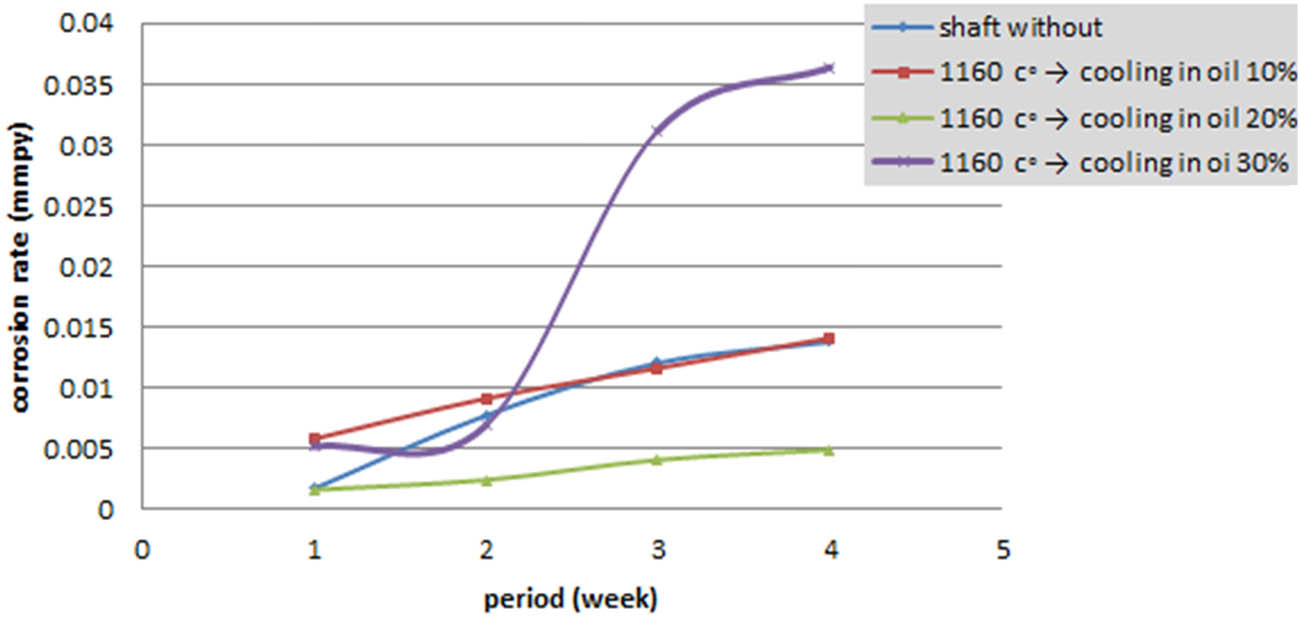
Corrosion rate for different cold working quenching in oil.

Corrosion rate for different cold working quenching in water.
3.5 GRG analysis using Taguchi
The main effects analysis is utilised to examine the influence and impacts of input parameters on the GRG, as shown in Figure 8. It is clear from Figure 8 that as CM changed from sea water to crude oil, the S/N ratio decreases [33]. Also the S/N ratio decreases when the HT is applied. But in the case of cold work, the S/N ratio also decreases and then increases at 30%. Figure 8 shows how to estimate CM at level 1, HT at level 1, and cold work at level 4, which means CM1-HT1-CW4 will concurrently give the optimal output characteristics (CR and surface hardness).
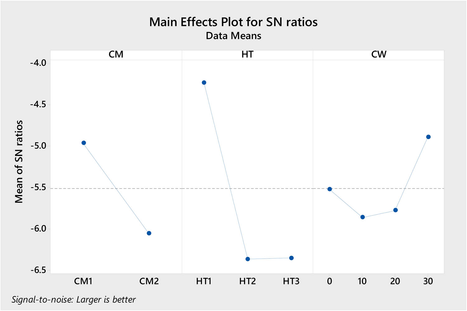
S/N ratio for GRG main influence plot.
3.5.1 Signal-to-noise ratio response table
Based on the rank value shown in Table 17, the response table shows that the control factors affecting the response variable (GRG) follow the prescribed sequence in descending order: HT > CM > CW.
S/N ratio response table (larger is better)
| Level | CM | HT | CW |
|---|---|---|---|
| 1 | −4.966 | −4.237 | −5.522 |
| 2 | −6.055 | −6.365 | −5.861 |
| 3 | −6.354 | −5.776 | |
| 4 | −4.890 | ||
| Delta | 1.090 | 2.128 | 0.971 |
| Rank | 2 | 1 | 3 |
3.5.2 Analysis of mean
The optimal amount for the process parameters was calculated using the analysis of means (ANOM). The collection of input parameters is presented in Figure 9’s ANOM graph for response variable optimisation (GRG). We must go with the higher values of input parameters under the larger, better criteria used for optimisation of GRG since we are improving the process parameters under multi-objective optimisation such that sea water may be used as the corrosive medium, without HT, and with 30% cold work, which is the ideal combination of input parameters.

Mean of means of GRG main effect plot.
The response table indicates that the control variables that affect the response variables follow a decreasing order HT > CW > CM based on the rank value presented in Table 18.
Response table for means
| Level | CM | HT | CW |
|---|---|---|---|
| 1 | 0.5715 | 0.6210 | 0.5310 |
| 2 | 0.5089 | 0.4882 | 0.5172 |
| 3 | 0.4845 | 0.5223 | |
| 4 | 0.5842 | ||
| Delta | 0.0626 | 0.1365 | 0.0670 |
| Rank | 3 | 1 | 2 |
3.6 Variance analysis for GRG
The P value for the HT parameters is less than 0.05, which is considered significant (lower probabilities give greater proof against the null hypothesis), and its percentage of contribution is also high, being 38.39%. This indicates that HT is the most important variable, followed by CW and CM, which have 16.87 and 8.64% influence, respectively, in the GRG ANOVA table. The F-value, a test statistic used to establish if a term is related to a response, also demonstrates that the HT is the aspect that has the greatest impact on the GRG response (Table 19).
Variance analysis
| Source | DF | Seq SS | Contribution (%) | Adj SS | Adj MS | F-Value | P-Value |
|---|---|---|---|---|---|---|---|
| CM | 1 | 0.01959 | 8.64 | 0.01959 | 0.019589 | 3.11 | 0.101 |
| HT | 2 | 0.08702 | 38.39 | 0.10840 | 0.054201 | 8.61 | 0.004 |
| CW | 3 | 0.03825 | 16.87 | 0.03825 | 0.012751 | 2.03 | 0.160 |
| Error | 13 | 0.08184 | 36.10 | 0.08184 | 0.006295 | ||
| Total | 19 | 0.22670 | 100.00 |
4 Conclusions
In this work, two techniques were used to strengthen AISI 316 stainless steel. In the first instance, the specimens were immersed in two hostile environments (crude oil and seawater) after having gone through many cold working actions on the tensile machine. In the second instance, the specimens were sliced before being heated. These samples were afterward subjected to the same circumstances as the initial case. The most important conclusions are as follows:
Cold action has been accompanied by stress-related twinning and austenite phase deformation, which resulted in fast grain splitting and the creation of an austenite and ferrite ribbon-type microstructure.
The hardness values increase in direct proportion to the intensity of cold working. Since a decline in hardness values was noticeable as a result of the microstructure changes that took place throughout the annealing process, it is also possible to see how the annealing HT affected hardness values.
The multi-objective optimisation technique we suggested reveals that HT is the element with the greatest influence, followed by CW and CM.
The order of the descending importance of the control variables impacting the response variable (GRG) is as stated: CW > HT > CM.
The combined set of the resultant parameters (CR and surface hardness) will be the best possible when CM are at level 1, HT is at level 1, and cold work is at level 4, which provided by CM1-HT1-CW4.
Acknowledgement
The writers would want to take this chance to say how grateful they are to the College of Engineering at the University of Basrah’s departments of mechanical engineering and materials engineering.
-
Funding information: The authors state no funding involved.
-
Author contributions: All authors have collectively accepted responsibility for the entire content of the manuscript and have given their approval for its submission. Basil Sh. Munahi and Haider Mahdi Lieth conceptualized and designed the study. Haider M. Mohammad and Haider Mahdi Lieth conducted the experiments, ensuring the robustness and reliability of the data. Basil Sh. Munahi developed and implemented the optimization model codes. All authors actively participated in critical discussions, providing valuable insights that shaped the research, data analysis, and manuscript composition.
-
Conflict of interest: Authors state the absence of any conflicts of interest.
-
Data availability statement: Data sharing is not applicable to this article as no datasets were generated or analysed during the current study.
References
[1] Li SX, He YN, Yu SR, Zhang PY. Evaluation of the effect of grain size on chromium carbide precipitation and intergranular corrosion of 316L stainless steel. Corros Sci. 2013;66:211–6.10.1016/j.corsci.2012.09.022Search in Google Scholar
[2] Chen J, Xiao Q, Lu Z, Ru X, Han G, Tian Y, et al. The effects of prior-deformation on anodic dissolution kinetics and pitting behavior of 316L stainless steel. Int J Electrochem Sci. 2016;11(2):1395–415.10.1016/S1452-3981(23)15930-XSearch in Google Scholar
[3] Tanhaei S, Gheisari KH, Alavi Zaree SR. Effect of cold rolling on the microstructural, magnetic, mechanical, and corrosion properties of AISI 316L austenitic stainless steel. Int J Min Metall Mater. 2018;25(6):630–40.10.1007/s12613-018-1610-ySearch in Google Scholar
[4] Shih CC, Shih CM, Su YY, Su LHJ, Chang MS, Lin SJ. Effect of surface oxide properties on corrosion resistance of 316L stainless steel for biomedical applications. Corros Sci. 2004;46(2):427–41.10.1016/S0010-938X(03)00148-3Search in Google Scholar
[5] Lodhi MJK, Deen KM, Greenlee-Wacker MC, Haider W. Additively manufactured 316L stainless steel with improved corrosion resistance and biological response for biomedical applications. Addit Manuf. 2019;27:8–19.10.1016/j.addma.2019.02.005Search in Google Scholar
[6] Tayyab KB, Farooq A, Alvi AA, Nadeem AB, Deen KM. Corrosion behavior of cold-rolled and post heat-treated 316L stainless steel in 0.9wt% NaCl solution. Int J Min Metall Mater. 2021;28(3):440–9.10.1007/s12613-020-2054-8Search in Google Scholar
[7] Milosan I, Florescu M, Cristea D, Voiculescu I, Pop MA, Cañadas I, et al. Evaluation of heat-treated AISI 316 stainless steel in solar furnaces to be used as possible implant material. Materials. 2020;13(3):581.10.3390/ma13030581Search in Google Scholar PubMed PubMed Central
[8] Muley SV, Vidvans AN, Chaudhari GP, Udainiya S. An assessment of ultra fine grained 316L stainless steel for implant applications. Acta Biomater. 2016;30:408–19.10.1016/j.actbio.2015.10.043Search in Google Scholar PubMed
[9] Lieth HM, Al-Sabur R, Jassim RJ, Alsahlani A. Enhancement of corrosion resistance and mechanical properties of API 5L X60 steel by heat treatments in different environments. J Eng Res. 2021;9:428–40.10.36909/jer.14591Search in Google Scholar
[10] Xu D, Wan X, Yu J, Xu G, Li G. Effect of cold deformation on microstructures and mechanical properties of austenitic stainless steel. Metals. 2018;8(7):522. 10.3390/met8070522.Search in Google Scholar
[11] Qin W, Li J, Liu Y, Yue W, Wang C, Mao Q, et al. Effect of rolling strain on the mechanical and tribological properties of 316 L stainless steel. J Tribol. 2018;141(2):438–63.10.1115/1.4041214Search in Google Scholar
[12] Song R, Ponge D, Raabe D, Speer JG, Matlock DK. Overview of processing, microstructure and mechanical properties of ultrafine grained bcc steels. Mater Sci Eng A. 2006;441(1–2):1–17.10.1016/j.msea.2006.08.095Search in Google Scholar
[13] Ravi Kumar B, Sharma S, Mahato B. Formation of ultrafine grained microstructure in the austenitic stainless steel and its impact on tensile properties. Mater Sci Eng A. 2011;528(6):2209–16.10.1016/j.msea.2010.11.034Search in Google Scholar
[14] Nakhaie D, Moayed MH. Pitting corrosion of cold rolled solution treated 17-4 PH stainless steel. Corros Sci. 2014;80:290–8.10.1016/j.corsci.2013.11.039Search in Google Scholar
[15] Peguet L, Malki B, Baroux B. Influence of cold working on the pitting corrosion resistance of stainless steels. Corros Sci. 2007;49(4):1933–48.10.1016/j.corsci.2006.08.021Search in Google Scholar
[16] Fyfe D, Shanahan CEA, Shreir LL. Atmospheric corrosion of Fe-Cu alloys and Cu-containing steels. Corros Sci. 1970;10(11):817–30.10.1016/S0010-938X(70)80005-1Search in Google Scholar
[17] Osozawa K, Engell HJ. The anodic polarization curves of iron-nickel-chromium alloys. Corros Sci. 1966;6:389–93.10.1016/S0010-938X(66)80022-7Search in Google Scholar
[18] Kim K, Park M, Jang J, Kim H, Moon HS, Lim DH, et al. Improvement of strength and impact toughness for cold-worked austenitic stainless steels using a surface-cracking technique. Metals. 2018;8(11):932.10.3390/met8110932Search in Google Scholar
[19] Lieth HM, Jabbar MA, Jassim RJ, Al-Sabur R. Optimize the corrosion behavior of AISI 204Cu stainless steel in different environments under previous cold working and welding. Metall Res Technol. 2023;120(4):415.10.1051/metal/2023058Search in Google Scholar
[20] E8/E8M-22. Standard test methods for tension testing of metallic materials. ASTM; 2022.Search in Google Scholar
[21] E384-17. Standard test method for microindentation hardness of materials. ASTM; 2021.Search in Google Scholar
[22] G31. Standard guide for laboratory immersion corrosion testing of metals. ASTM; 2021.Search in Google Scholar
[23] Saini N, Dhingra DS. Tools and techniques used in optimization of machining parameters in CNC lathe turning of aluminium 7075 alloy. 2018;4:30–8.Search in Google Scholar
[24] Yan FK, Liu GZ, Tao NR, Lu K. Strength and ductility of 316L austenitic stainless steel strengthened by nano-scale twin bundles. Acta Mater. 2012;60(3):1059–71.10.1016/j.actamat.2011.11.009Search in Google Scholar
[25] Asokan P, Ravi Kumar R, Jeyapaul R, Santhi M. Development of multi-objective optimization models for electrochemical machining process. Int J Adv Manuf Technol. 2008 Oct;39(1–2):55–63.10.1007/s00170-007-1204-8Search in Google Scholar
[26] Kolahan F, Golmezerji R, Moghaddam MA. Multi objective optimization of turning process using grey relational analysis and simulated annealing algorithm. Appl Mech Mater. 2012;110–116:2926–32.10.4028/www.scientific.net/AMM.110-116.2926Search in Google Scholar
[27] Yan J, Li L. Multi-objective optimization of milling parameters – the trade-offs between energy, production rate and cutting quality. J Clean Prod. 2013;52:1–10.10.1016/j.jclepro.2013.02.030Search in Google Scholar
[28] Jayaraman P, Kumar LM. Multi-response optimization of machining parameters of turning AA6063 T6 aluminium alloy using grey relational analysis in Taguchi method. Procedia Eng. 2014;97:197–204.Search in Google Scholar
[29] Hug E, Prasath Babu R, Monnet I, Etienne A, Moisy F, Pralong V, et al. Impact of the nanostructuration on the corrosion resistance and hardness of irradiated 316 austenitic stainless steels. Appl Surf Sci. 2017;392:1026–35.10.1016/j.apsusc.2016.09.110Search in Google Scholar
[30] Hou XZ, Zheng WJ, Song ZG, Long JM. Effect of cold work on structure and mechanical behavior of 316L stainless steel. J. Iron Steel Res. 2013;25:53–7.Search in Google Scholar
[31] Raykar SJ, D’Addona DM, Mane AM. Multi-objective optimization of high speed turning of Al 7075 using grey relational analysis. Procedia CIRP. 2015;33:293–8.10.1016/j.procir.2015.06.052Search in Google Scholar
[32] E407. Standard practice for microetching metals and alloys. United States: ASTM International; 2012. p. 19428–2959.Search in Google Scholar
[33] Jayaraman P, Mahesh Kumar L. Multi-response optimization of machining parameters of turning AA6063 T6 aluminium alloy using grey relational analysis in Taguchi method. Procedia Engineering. 2014;97:197–204.10.1016/j.proeng.2014.12.242Search in Google Scholar
© 2024 the author(s), published by De Gruyter
This work is licensed under the Creative Commons Attribution 4.0 International License.
Articles in the same Issue
- Editorial
- Focus on NLENG 2023 Volume 12 Issue 1
- Research Articles
- Seismic vulnerability signal analysis of low tower cable-stayed bridges method based on convolutional attention network
- Robust passivity-based nonlinear controller design for bilateral teleoperation system under variable time delay and variable load disturbance
- A physically consistent AI-based SPH emulator for computational fluid dynamics
- Asymmetrical novel hyperchaotic system with two exponential functions and an application to image encryption
- A novel framework for effective structural vulnerability assessment of tubular structures using machine learning algorithms (GA and ANN) for hybrid simulations
- Flow and irreversible mechanism of pure and hybridized non-Newtonian nanofluids through elastic surfaces with melting effects
- Stability analysis of the corruption dynamics under fractional-order interventions
- Solutions of certain initial-boundary value problems via a new extended Laplace transform
- Numerical solution of two-dimensional fractional differential equations using Laplace transform with residual power series method
- Fractional-order lead networks to avoid limit cycle in control loops with dead zone and plant servo system
- Modeling anomalous transport in fractal porous media: A study of fractional diffusion PDEs using numerical method
- Analysis of nonlinear dynamics of RC slabs under blast loads: A hybrid machine learning approach
- On theoretical and numerical analysis of fractal--fractional non-linear hybrid differential equations
- Traveling wave solutions, numerical solutions, and stability analysis of the (2+1) conformal time-fractional generalized q-deformed sinh-Gordon equation
- Influence of damage on large displacement buckling analysis of beams
- Approximate numerical procedures for the Navier–Stokes system through the generalized method of lines
- Mathematical analysis of a combustible viscoelastic material in a cylindrical channel taking into account induced electric field: A spectral approach
- A new operational matrix method to solve nonlinear fractional differential equations
- New solutions for the generalized q-deformed wave equation with q-translation symmetry
- Optimize the corrosion behaviour and mechanical properties of AISI 316 stainless steel under heat treatment and previous cold working
- Soliton dynamics of the KdV–mKdV equation using three distinct exact methods in nonlinear phenomena
- Investigation of the lubrication performance of a marine diesel engine crankshaft using a thermo-electrohydrodynamic model
- Modeling credit risk with mixed fractional Brownian motion: An application to barrier options
- Method of feature extraction of abnormal communication signal in network based on nonlinear technology
- An innovative binocular vision-based method for displacement measurement in membrane structures
- An analysis of exponential kernel fractional difference operator for delta positivity
- Novel analytic solutions of strain wave model in micro-structured solids
- Conditions for the existence of soliton solutions: An analysis of coefficients in the generalized Wu–Zhang system and generalized Sawada–Kotera model
- Scale-3 Haar wavelet-based method of fractal-fractional differential equations with power law kernel and exponential decay kernel
- Non-linear influences of track dynamic irregularities on vertical levelling loss of heavy-haul railway track geometry under cyclic loadings
- Fast analysis approach for instability problems of thin shells utilizing ANNs and a Bayesian regularization back-propagation algorithm
- Validity and error analysis of calculating matrix exponential function and vector product
- Optimizing execution time and cost while scheduling scientific workflow in edge data center with fault tolerance awareness
- Estimating the dynamics of the drinking epidemic model with control interventions: A sensitivity analysis
- Online and offline physical education quality assessment based on mobile edge computing
- Discovering optical solutions to a nonlinear Schrödinger equation and its bifurcation and chaos analysis
- New convolved Fibonacci collocation procedure for the Fitzhugh–Nagumo non-linear equation
- Study of weakly nonlinear double-diffusive magneto-convection with throughflow under concentration modulation
- Variable sampling time discrete sliding mode control for a flapping wing micro air vehicle using flapping frequency as the control input
- Error analysis of arbitrarily high-order stepping schemes for fractional integro-differential equations with weakly singular kernels
- Solitary and periodic pattern solutions for time-fractional generalized nonlinear Schrödinger equation
- An unconditionally stable numerical scheme for solving nonlinear Fisher equation
- Effect of modulated boundary on heat and mass transport of Walter-B viscoelastic fluid saturated in porous medium
- Analysis of heat mass transfer in a squeezed Carreau nanofluid flow due to a sensor surface with variable thermal conductivity
- Navigating waves: Advancing ocean dynamics through the nonlinear Schrödinger equation
- Experimental and numerical investigations into torsional-flexural behaviours of railway composite sleepers and bearers
- Novel dynamics of the fractional KFG equation through the unified and unified solver schemes with stability and multistability analysis
- Analysis of the magnetohydrodynamic effects on non-Newtonian fluid flow in an inclined non-uniform channel under long-wavelength, low-Reynolds number conditions
- Convergence analysis of non-matching finite elements for a linear monotone additive Schwarz scheme for semi-linear elliptic problems
- Global well-posedness and exponential decay estimates for semilinear Newell–Whitehead–Segel equation
- Petrov-Galerkin method for small deflections in fourth-order beam equations in civil engineering
- Solution of third-order nonlinear integro-differential equations with parallel computing for intelligent IoT and wireless networks using the Haar wavelet method
- Mathematical modeling and computational analysis of hepatitis B virus transmission using the higher-order Galerkin scheme
- Mathematical model based on nonlinear differential equations and its control algorithm
- Bifurcation and chaos: Unraveling soliton solutions in a couple fractional-order nonlinear evolution equation
- Space–time variable-order carbon nanotube model using modified Atangana–Baleanu–Caputo derivative
- Minimal universal laser network model: Synchronization, extreme events, and multistability
- Valuation of forward start option with mean reverting stock model for uncertain markets
- Geometric nonlinear analysis based on the generalized displacement control method and orthogonal iteration
- Fuzzy neural network with backpropagation for fuzzy quadratic programming problems and portfolio optimization problems
- B-spline curve theory: An overview and applications in real life
- Nonlinearity modeling for online estimation of industrial cooling fan speed subject to model uncertainties and state-dependent measurement noise
- Quantitative analysis and modeling of ride sharing behavior based on internet of vehicles
- Review Article
- Bond performance of recycled coarse aggregate concrete with rebar under freeze–thaw environment: A review
- Retraction
- Retraction of “Convolutional neural network for UAV image processing and navigation in tree plantations based on deep learning”
- Special Issue: Dynamic Engineering and Control Methods for the Nonlinear Systems - Part II
- Improved nonlinear model predictive control with inequality constraints using particle filtering for nonlinear and highly coupled dynamical systems
- Anti-control of Hopf bifurcation for a chaotic system
- Special Issue: Decision and Control in Nonlinear Systems - Part I
- Addressing target loss and actuator saturation in visual servoing of multirotors: A nonrecursive augmented dynamics control approach
- Collaborative control of multi-manipulator systems in intelligent manufacturing based on event-triggered and adaptive strategy
- Greenhouse monitoring system integrating NB-IOT technology and a cloud service framework
- Special Issue: Unleashing the Power of AI and ML in Dynamical System Research
- Computational analysis of the Covid-19 model using the continuous Galerkin–Petrov scheme
- Special Issue: Nonlinear Analysis and Design of Communication Networks for IoT Applications - Part I
- Research on the role of multi-sensor system information fusion in improving hardware control accuracy of intelligent system
- Advanced integration of IoT and AI algorithms for comprehensive smart meter data analysis in smart grids