Fast analysis approach for instability problems of thin shells utilizing ANNs and a Bayesian regularization back-propagation algorithm
-
T. N. Nguyen
 ,
Dongsheng Zhang
,
Dongsheng Zhang

Abstract
This research develops a data-driven methodology for structural instability problems with highly nonlinear, difficult, noisy, and small data. A fast analysis and prediction (FAP) approach for instability problems of thin shells is first proposed. This approach contains two phases: the fast numerical analysis and the pure prediction utilizing artificial neural networks (ANNs) incorporated with the Bayesian regularization (B-R) algorithm as follows: (1) in Phase 1 (the fast numerical analysis), post-buckling analysis is conducted utilizing a minor amount of load steps. The load–displacement relation achieved from Phase 1 is not exact because of the small number of load steps utilized; (2) in Phase 2 (the prediction), the loads and deflections achieved from Phase 1 were employed as the data for training ANNs. The trained networks, including the load and displacement networks, were employed to fast predict loads and deflections at any step of the post-buckling analysis. After utilizing Phase 2, a smooth, complete and exact load–displacement curve was achieved. In Phase 1, the available formulation for post-buckling analysis of thin shells in the literature was utilized. Five popular types of instabilities chosen to confirm the effectiveness and exactness of the FAP were snap-through, snap-back, softening–hardening, kink instabilities, and delamination buckling and post-buckling of composites. The high exactness and effectiveness of the FAP were confirmed in the numerical verification section. The present approach saves a huge computation compared to the other ones. It was found that ANNs incorporated with the B-R algorithm have notable advantages compared to numerous neural networks. The proposed approach is applicable to simulations or experiments where data are “expensive”, highly nonlinear, difficult, and limited. Utilizing the proposed approach for these fields can dramatically save time and money.
1 Introduction
A structure under a compressive load can present an instability phenomenon. When the compressive load is large enough or reaches the buckling load, the structure can reduce its stiffness, experience a notable change in geometry, and become unstable. When instability occurs, the structure can reduce its load-carrying capacity and is incapable of maintaining a stable equilibrium configuration. Investigations into structural instability and post-buckling behavior are necessary and play an important role in structural engineering, especially when post-buckling behavior is unpredictable. Load–displacement equilibrium paths are usually employed to evaluate structural instability. Several approaches, such as an analytical approach, a semi-analytical approach, and a numerical approach, can be employed to obtain those equilibrium paths. The numerical approach is convenient and powerful. It is applicable to problems with complex loading, boundaries, and geometries. Therefore, it is popularly employed in both academic and industrial problems. Utilizing the numerical approach for solving an instability problem needs a complete combination of an appropriate formulation, a numerical technique, and a nonlinear solver. One of the difficulties of solving instability problems utilizing the numerical approach is high time-consuming because of a huge computation and numerous computational iterations. This reality is clearly seen in large-scale problems utilizing thousands or millions degrees of freedom. Another difficulty in solving instability problems is divergent in some cases, especially when the equilibrium path passes the limit or special points, the inflection points. To overcome the aforementioned difficulties, a lot of approaches, nonlinear solvers, and techniques were proposed to decrease the number of computational iterations and to successfully pass limit or special points on the equilibrium paths including the Newton–Raphson (N-R) technique [1], the modified N-R [2], the modified Riks (M–R) technique [3], the iterative techniques upon an optimization technique [4] and upon residual areas [5], the Koiter (K) technique [6], the accelerated K technique [7], the Koiter-Newton (K-N) technique [8,9], a new technique upon the discretization of governing equations [10], a general path-following methodology [11], the methodology that improves effectiveness of the Newton technique [12], the dynamic relaxation techniques [13,14], a technique without utilizing the predictor [15], and the multi-point techniques [16]. Although numerous nonlinear solvers, approaches, and techniques have been developed and proposed, high time-consuming is still a difficulty in solving instability problems utilizing the numerical approach. To completely overcome this disadvantage, the FAP for instability problems of thin shells is proposed in this work. The present approach includes two phases: the fast analysis utilizing pure isogeometric analysis (IGA) and the prediction utilizing ANNs. In Phase 1, a post-buckling analysis is conducted utilizing a minor amount of load steps. In Phase 2, the obtained data from Phase 1 are utilized to train ANNs to fast and completely predict post-buckling behavior of the structure for many load steps. Interestingly, the computational cost of the FAP is dramatically lower than that of other ones.
ANNs are computing systems simulated according to the operation of biological neurons in the human brain. An ANN is a group of connected neurons. An ANN can mimic a human brain to fast and simply resolve complex problems that possess nonlinear relationships [17]. Up to now, ANNs have been successfully used in many areas, including bridge deck structure [18], optimal material structure [19], aircraft design [20], prediction of the fracture energy of concrete [21], buckling capacity assessment of steel structures [22], compressive strength prediction of cement [23], an optimization for hydrogen purification performance [24], an optimization for fatigue prediction [25], structural damage identification [26], and damage detection [27]. For nonlinear problems utilizing the numerical methodology, ANNs were employed to improve an algorithm for nonlinear dynamic analysis [28] and the Newton iterative technique [29]. Recently, the FAP for nonlinear bending analysis of structures was proposed [30], in which, N-R technique was applied to solve the nonlinear equation system in Phase 1. In the study by Nguyen et al. [30], the approach was proposed and investigated for pure bending problems of plates/shells. As known, loads are priorly known in the bending problems, while displacements are unknown. Thus, ANNs incorporated with the B-R algorithm were only employed to predict series of displacements in Phase 2 in the study by Nguyen et al. [30]. In this study, the FAP is proposed for instability problems of thin shells. As known, solving instability problems is much difficult than solving nonlinear bending problems because the equilibrium path can pass the limit or special points, the inflection points. Solving instability problems can be divergent in some cases. Thus, in this study, a powerful nonlinear solver named the modified Riks technique is applied to solve the nonlinear equation system in Phase 1. Besides different from the nonlinear bending problems, loads and displacements are both unknown in the instability problems. Thus, ANNs incorporated with the B-R algorithm are employed to predict the series of displacements and loads in Phase 2. It is emphasized that the present approach employs a minor amount of data points in the training phase. Thus, the time for training a network is very small and can be neglected in evaluating the effectiveness of the proposed approach. The idea of this work is simple in its implementation and can dramatically save computation compared to the another approach. The size of the dataset in this work is relatively small. Both deep neural networks (DNNs) including multiple hidden layers and artificial neural networks (ANNs) including one hidden layer can be used for training. However, we chose ANNs combined with Bayesian regularization back-propagation (BPP) algorithm because of their computational efficiency compared to DNNs. Training a DNN is usually longer than an ANN. This can be explained as follows. DNNs use multiple hidden layers and many neurons on each layer. Thus, there are many computations in each layer, and the weight optimization is more complex and longer. Inversely, ANNs use only one hidden layer, and so time for training is shorter than that for DNNs. However, we recommend using DNNs if the size of dataset is large, for example, 10,000 data points or more. For such big data, DNNs are more accurate than ANNs in predictions. Structure of this article is organized as follows. The next section shows post-buckling analysis of isotropic thin shells utilizing the first-order shear deformation shell theory (FSDT). Section 3 presents the isotropic shell formulation for post-buckling analysis utilizing FSDT and IGA. The FAP for instability problems of thin shells is presented in Section 4. The numerical verification is shown in Section 5. Finally, several notable conclusions are drawn.
2 Post-buckling analysis of isotropic shells utilizing FSDT
The aim of this article is to propose a fast analysis and prediction (FAP) approach for instability problems. Without losing the generality of the proposed approach, shell instabilities were chosen to confirm the effectiveness and exactness of the approach. For the analysis employed in Phase 1, the current formulation was reemployed from a published article on post-buckling analysis of shells. Therefore, a brief formulation of the analysis is presented in this article. The nonlinearity of the shell formulation is established upon the von Karman hypothesis. We now consider an isotropic shell depicted in Figure 1. The shell strain vectors upon the FSDT are
where
where
where
where the in-plane stress vector is
The bending and shear stress vectors, respectively, are

Panel subjected to a radial pressure.
For isotropic shells, the generalized strain vector
where
where
3 Isotropic shell formulation for post-buckling analysis utilizing FSDT and IGA
This part briefly presents the post-buckling analysis of isotropic shells upon FSDT and IGA. As introduced earlier, the detailed formulation can be found in the study for the post-buckling analysis of functionally graded carbon nanotube-reinforced composite (FG-CNTRC) shells utilizing FSDT and IGA. As known, an isotropic shell is a separate case of an FG-CNTRC shell. Therefore, the formulation for isotropic shells is the same as for FG-CNTRC shells, except there is a small difference in determining the matrices for material presented in Eqs (10)–(12). At the
where the tangent stiffness matrix is
and the load vector
where
where
In this article, the modified Riks technique [3] is employed to solve the system of linear incremental equations. With an arbitrary load increment, an iterative process is performed until the following convergence criterion is satisfied as
Once the incremental solutions are achieved from Eq. (13), the load factor
where
4 FAP approach for instabilities of thin shells
4.1 Brief introduction to ANNs
ANNs are systems simulated according to the operation of biological neurons in the human brain [21,31]. An ANN is a group of connected nodes as depicted in Figure 2(a). In this network, signals are spread from these neurons to those neurons via connections. Each neuron in the network has a weight adjusted during the learning process. The weight may decrease and increase the signal strength at the connection. During the learning process, the signals are transmitted from the first layer to the last layer numerous times until optimization of all the weights is achieved. The neuron’s output is computed via the function (
where
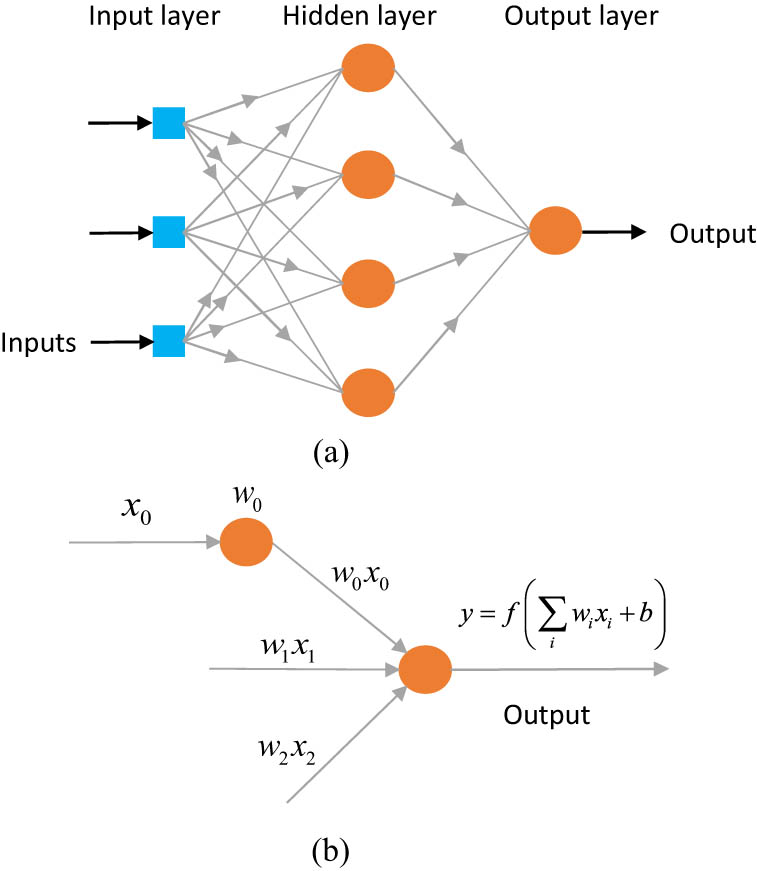
Typical architecture and output calculation of an ANN: (a) architecture of a typical ANN and (b) calculating output for a neuron with three inputs.
ANNs are established upon the feed-forward BPP algorithm. In application, the input data together with the desired output data are first provided for ANNs. Then, the neuron’s weight and bias are modified (once or many times) to decrease the distinction between the actual and desired outputs of the network. The target of training ANNs is to minimize network error (the distinction between the actual output and the desired output of the network) or optimize the performance of the networks in predictions. The training process can end when the stopping criterion upon the mean square error (MSE) is met. The MSE is calculated as [21,31]
where
Several optimization techniques can be employed to speed up the convergence of the BPP algorithm including the scaled conjugate gradient (SCG) technique, the B-R technique, and the Levenberg–Marquardt (L-M) technique. The details of these optimization techniques can be found in previous studies [21,31]. For all the networks in this article, the B-R technique is utilized.
4.2 B-R BPP algorithm
The objective function of ANNs utilizing B-R is written as [32]
where
where
where
In the B-R BPP algorithm, the optimal weights are found when the posterior probability
We assume that the prior density
Note that all the probabilities have a Gaussian form. Thus, Eq. (29) can be re-expressed as
where
where
(0) Initialize the weights
(1) Employ the L-M algorithm for finding the minimum of the objective function.
(2) Calculate
(3) Compute new values of
(4) Steps 1–3 are iterated until we obtain the convergence.
where
4.3 FAP approach for instability problems of thin shells
Some popular types of thin shell instabilities chosen to confirm the effectiveness and exactness of the FAP were snap-through, snap-back, kink, and softening–hardening instabilities. One of the great difficulties of solving structural instability problems is highly time-consuming because of numerous computational iterations and a huge computation. This reality is clearly seen in large-scale problems utilizing thousands or millions of degrees of freedom. Another difficulty in solving instability problems is divergence in many cases especially when the equilibrium path passes the limit points, the inflection points, the neighborhoods of turning points, and bifurcations. To overcome the aforementioned difficulties, the FAP for instability problems of thin shells is proposed in this article. It is noted that in instability or post-buckling analysis of structures, loads and displacement vectors of analysis steps are unknown. The present methodology contains two phases: fast numerical analysis and pure prediction utilizing ANNs as follows: (1) for Phase 1, post-buckling analysis is conducted utilizing a minor amount of load steps. The obtained load–displacement relation is not exact because of a minor amount of load steps utilized; (2) for Phase 2, the loads and the deflections obtained from Phase 1 are considered as the data for training networks. Then, the trained networks, including the load network and the displacement network, are utilized to fast predict loads and deflections at any step of the post-buckling analysis. Upon utilizing Phase 2, an exact and smooth load–displacement curve is achieved. Figures 3 and 4, respectively present the description and the flowchart of the FAP. The numerical verification section demonstrates the high exactness and effectiveness of the FAP for instability problems. Besides, the high ability of the FAP to detect limit and inflection points is also confirmed in the next section.
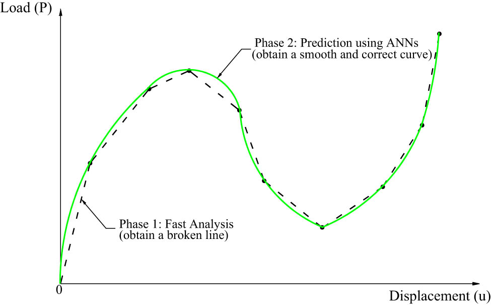
FAP for instability problems utilizing ANNs.

Workflow of the present methodology for instability problems.
5 Numerical verification
The effectiveness and exactness of the present approach for instability problems of thin shells are verified in this section. Without losing the generality of the proposed approach, four popular types of thin shell instabilities chosen to confirm the effectiveness and exactness of the present approach were snap-through, snap-back, kink and softening–hardening instabilities. For convenience and consistency, the following parameters are fixed for the whole manuscript.
For the analysis in Phase 1, the computational models are analyzed utilizing 14 × 14 cubic elements. The hinged boundary is described as
For the prediction packages in Phase 2, the structure of all ANNs includes the hidden and output layers. The number of neurons in the first and second layers is 15 and 1, respectively. ANNs utilizing the B-R BPP algorithm did not require a validation dataset to evaluate the models. The algorithm has a built-in validation technique. Therefore, in the training phase, the dataset was separated into two data groups: the training data (
All the networks were trained utilizing the NN-fitting application built in MATLAB R2021a. The ANN’s parameters and architecture are listed in table 1 in the study by Nguyen et al. [30].
For verification study, the results of the FAP are compared with that of pure IGA and reference solutions. The pure IGA is conducted utilizing the same formulation as the FAP but needs much more load steps.
5.1 FAP approach for snap-through instability problems of thin shells
The effectiveness and exactness of the FAP for snap-through instability problems of shells and the performance of ANNs incorporated with the B-R are studied in this subsection. We consider a hinged-hinged isotropic cylindrical panel under a central point load, as in Figure 5. The geometric data and the material properties of the panel are provided at the beginning of this section. Note that in this problem, the panel thickness is
For the training process of the displacement network, the data sizes of the input, output, and target are equal. The number of load steps in Phase 1 is 13. Thirteen achieved deflections are utilized as the target data for training the displacement network. For training networks, we utilize a typical input data as
For the application of the displacement network: if we need to predict full deflections of 31 equal load steps utilizing the trained ANN, the input is still from 1 to 14 but the increment in the data is
The training process and the application of the load network are the same as that of the displacement network. The details can be found in Figure 8.

Hinged-hinged panel under a point load at the center.

Analysis of the hinged-hinged panel utilizing the FAP: Phase 1 (fast analysis, 13 load steps),

Data structure of the first and second phases for displacement prediction.

Data structure of the first and second phases for load prediction.
Figure 9 presents the training performance of the displacement and load networks. The training processes of the two networks can be, respectively, stopped after 443 and 99 epochs because the MSEs are very small. The results of applications of the trained ANNs are presented in Figure 10. The very good agreements are found between the obtained outputs (from the networks) and the targets (from pure IGA). The networks are well trained. Interestingly, the cost for training and application of a network is very low (approximately 3 seconds) because the sizes of data are very small together with the advantages of ANNs. Thus, this cost is neglected in evaluation of the effectiveness of the FAP. Besides, Figure 11 presents the obtained results of the FAP utilizing 13 fast analysis steps in the comparison with that of pure IGA utilizing 31 load steps and that of Sabir and Djoudi [33] utilizing pure finite element (FE) analysis with 31 load steps. These results match well. A smooth, complete, and exact curve is achieved after utilizing Phase 2. Also, the upper and lower limit points are detected successfully upon ANNs. The present approach saves 58% of the computational effort compared to other approaches. The high effectiveness and exactness of the present approach are verified. Figure 12 describes the effect of the number of fast analysis steps on the solution. The higher number of fast analysis steps, the higher exactness of the FAP solution. Utilizing 13 analysis steps in Phase 1 can produce a great solution that balances exactness and effectiveness. For snap-through instability problems, we recommend to utilize the present approach with 13 fast analysis steps to ensure exactness and effectiveness in solutions.

Training performance of ANNs in Phase 2: (a) for displacement network and (b) for load network.

Applying the trained networks in Phase 2: (a) for displacement (mm) network and (b) for load (kN) network.

Central deflection of the hinged-hinged panel utilizing various approaches,

Number of fast analysis steps affects the FAP solution for a hinged-hinged panel,
5.2 FAP approach for softening–hardening instability problems of shells
The hinged-hinged panel under a central point load depicted in Figure 5 is continued considering. The geometric data and the material data of the panel are unchanged, except the panel thickness in this problem is

Analysis of the hinged-hinged panel utilizing the FAP: Phase 1 (fast analysis, seven load steps),

Central deflection of the hinged-hinged panel utilizing various approaches,

Number of fast analysis steps affects the FAP solution for a hinged-hinged panel,
5.3 FAP approach for snap-back instability problems of shells
In the this problem, the clamped-hinged panel under a central point load depicted in Figure 16 is considered. The geometric data and material data of the panel are the same as those in the first problem, except the panel thickness, in this case, is

Clamped-hinged panel under a central load,

Analysis of the clamped-hinged panel utilizing the FAP: Phase 1 (fast analysis, 14 load steps),

Central deflection of the clamped-hinged panel utilizing various approaches,

Number of fast analysis steps affects the FAP solution for a clamped-hinged panel,
ANNs incorporated with the B-R algorithm recommended for the FAP have some notable advantages compared to numerous existing networks. To confirm this, we solved this problem utilizing different types of NNs in Phase 2 including ANNs incorporated with the L-M algorithm [21,31], ANNs incorporated with the SCG algorithm [21,31], DNNs [34], and the group method of data handling (GMDH) [35]. For this problem, the data obtained in Phase 1 were re-utilized for training networks in Phase 2. Notably, the ANN’s structure, which includes number of neurons and layers, is unchanged. The change is the SCG algorithm, and the L-M algorithm is utilized in this investigation. All the ANNs were trained utilizing MATLAB R2021a as mentioned earlier. For all types of networks in this investigation and in this article, data splitting is performed as follows: the training set (70%), the testing set (15%), and the validation set (15%). Group method of data handling is utilized in many fields including forecasting, optimization, and pattern recognition. In this article, a GMDH-based NN [35] includes 15 neurons per layer and 4 hidden layers. We choose the selection pressure factor

Applications of the networks utilizing ANNs and the L-M algorithm: (a) network for displacement (mm) prediction and (b) network for load (kN) prediction.

Applications of the networks utilizing ANNs and the SCG algorithm: (a) network for displacement (mm) prediction and (b) network for load (kN) prediction.

Applications of the networks utilizing the GMDH: (a) network for displacement (mm) prediction and (b) network for load (kN) prediction.

Training performances of DNNs: (a) network for displacement prediction and (b) network for load prediction.

Applications of the trained networks utilizing the DNNs: (a) network for displacement (mm) prediction and (b) network for load (kN) prediction.

Analysis of a clamped-hinged panel utilizing the FAP and different NNs.

Network’s architecture affects the FAP solution: (a) number of neurons, data-splitting ratio: 85%, 15% and (b) data-splitting ratio (training, testing), 15 neurons in the hidden layer.
5.4 FAP approach for kink instability problems of shells
The panel in Figure 5 and Section 5.1 is continued considering. In this problem, the panel thickness is
![Figure 27
Analysis of the hinged-hinged composite panel with
h
h
= 6.35 mm and [
0
0
∕
9
0
0
∕
0
0
{0}^{0}/9{0}^{0}/{0}^{0}
] stacking sequence utilizing the FAP: (a) Phase 1 (fast analysis) and (b) Phase 2 (prediction) and comparison.](/document/doi/10.1515/nleng-2024-0012/asset/graphic/j_nleng-2024-0012_fig_027.jpg)
Analysis of the hinged-hinged composite panel with
5.5 FAP approach for an experiment
In the last problem, the FAP is applied to predict delamination buckling and post-buckling of composite laminates utilizing data from experiment. The compression test was conducted on HYE-3574 OH graphite/epoxy composites with built-in delamination [39]. The material properties are found in table 1 in the study by Gu and Chattopadhyay [39]. Geometry of specimen and compression test setup are shown in Figure 28 and Figure 4 in the study by Gu and Chattopadhyay [39], respectively. The delamination length is 3.0 in. The ply stacking sequence of the test specimen was
![Figure 28
An experiment of delamination postbuckling of composite laminates: Geometry of specimen [39].](/document/doi/10.1515/nleng-2024-0012/asset/graphic/j_nleng-2024-0012_fig_028.jpg)
An experiment of delamination postbuckling of composite laminates: Geometry of specimen [39].

Postbuckling path for the test specimen utilizing the FAP: (a) Phase 1 and (b) Phase 2 (prediction) and comparison.
Finally, the computational effectiveness of the FAP for various types of instabilities of thin shells is summarized and presented in Tables 1 and 2. It is concluded that utilizing the FAP can save a huge amount of computation compared to the other ones (fully pure isogeometric and fully pure FE analyses) and the experiment. Notably, the computational costs for problems of kink instability and experiment were not available in the literature [38,39]. Therefore, these costs are not present in Table 2.
Effectiveness of the FAP according to load steps
| Instabilities | Total steps per analysis | Saved computation (%) compared | |
|---|---|---|---|
| Pure analysis | FAP approach | with pure analysis approach | |
| Snap-through | 31 | 13 | 58 |
| Softening–hardening | 14 | 7 | 50 |
| Snap–back | 43 | 14 | 67 |
| Kink | 36 | 18 | 50 |
| Experiment | 19 | 10 | 47 |
Effectiveness of the FAP according to computational cost
| Instabilities | Total cost per analysis (s) | Saved cost (%) compared | |
|---|---|---|---|
| Pure analysis | FAP approach | with pure analysis approach | |
| Snap-through | 261 | 126 | 52 |
| Softening-hardening | 116 | 64 | 45 |
| Snap-back | 403 | 132 | 67 |
6 Conclusions
An FAP approach for instability problems of thin shells has been proposed. The present approach contains two phases: fast analysis and pure prediction. (1) for Phase 1, fast post-buckling analysis is conducted utilizing a minor amount of load steps. The obtained load–displacement relation from Phase 1 is incomplete and not exact because of a minor amount of load steps utilized; (2) for Phase 2, the loads and the deflections obtained from Phase 1 are considered as the data for training ANNs incorporated with Bayesian regularization (B-R). After that, the trained networks, including the load network and the displacement network, are utilized to fast predict load and deflection at any step of the post-buckling analysis. After utilizing Phase 2, an exact, complete, and smooth load–displacement curve is achieved. Interestingly, the cost for training and application of an ANN is very low (approximately 3 s) because the utilized data sizes are very small together with the advantages of ANNs. From the numerical verification, several notable conclusions are drawn as follows:
Good agreement between the results of the FAP and the reference results was found for all problems in this work. The present approach saves a huge computation compared to other ones. High effectiveness and exactness of the proposed approach for post-buckling analysis of thin shells were demonstrated.
The FAP solutions for instability problems are stable and exact. The more number of fast analysis steps, the more exact solution but high computational cost is required.
To produce good solutions for the FAP with a balance between exactness and effectiveness (the lowest computational cost), some conclusions are drawn as follows: For snap-through instability problems, we recommend to utilize the present approach with 13 load steps in Phase 1. For softening–hardening instability problems, we recommend to utilize the present approach with seven load steps in Phase 1. For snap-back instability problems, we recommend to utilize the present approach with 14 load steps in Phase 1.
ANNs incorporated with B-R, which are recommended for the present approach, have some notable advantages compared to numerous existing networks. We recommend to utilize ANNs incorporated with B-R in Phase 2 to achieve exact predictions. Besides, we recommend to utilize the present approach with the network’s architecture as: at least 85% data for training and 15 neurons in the hidden layer.
The FAP is applicable to experiments and highly nonlinear problems, which can have a kink on their equilibrium paths. This can save labor, time, and money for the experiments.
-
Funding information: This research project was supported by the Second Century Fund (C2F), Chulalongkorn University.
-
Author contributions: All authors have accepted responsibility for the entire content of this manuscript and approved its submission.
-
Conflict of interest: The authors state no conflict of interest.
-
Data availability statement: The datasets generated during and analyzed during the current study are available from the corresponding author on reasonable request.
References
[1] Zhang LW, Lei ZX, Liew KM, Yu JL. Large deflection geometrically nonlinear analysis of carbon nanotube-reinforced functionally graded cylindrical panels. Comput Meth Appl Mech Eng. 2014;273:1–18. 10.1016/j.cma.2014.01.024Search in Google Scholar
[2] Crisfield MA. A faster modified Newton-Raphson iteration. Comput Meth Appl Mech Eng. 1979;20(3):267–78. 10.1016/0045-7825(79)90002-1Search in Google Scholar
[3] Crisfield MA. A fast incremental/iterative solution procedure that handles ‘snap-through. Comput Struct. 1981;13(1):55–62. 10.1016/0045-7949(81)90108-5Search in Google Scholar
[4] Rezaiee-Pajand M, Naserian R. Geometrical nonlinear analysis based on optimization technique. Appl Math Model. 2018;53:32–48. 10.1016/j.apm.2017.08.003Search in Google Scholar
[5] Rezaiee-Pajand M, Naserian R. Using residual areas for geometrically nonlinear structural analysis. Ocean Eng. 2015;105:327–35. 10.1016/j.oceaneng.2015.06.043Search in Google Scholar
[6] Castro SGP, Jansen EL. Displacement-based formulation of Koiter’s method: Application to multi-modal post-buckling finite element analysis of plates. Thin-Walled Struct. 2021;159:107217. 10.1016/j.tws.2020.107217Search in Google Scholar
[7] Sun Y, Tian K, Li R, Wang B. Accelerated Koiter method for post-buckling analysis of thin-walled shells under axial compression. Thin-Walled Struct. 2020;155:106962. 10.1016/j.tws.2020.106962Search in Google Scholar
[8] Liang K, Ruess M, Abdalla M. The Koiter-Newton approach using von xxxx kinematics for buckling analyses of imperfection sensitive structures. Comput Meth Appl Mech Eng. 2014;279:440–68. 10.1016/j.cma.2014.07.008Search in Google Scholar
[9] Magisano D, Liang K, Garcea G, Leonetti L, Ruess M. An efficient mixed variational reduced-order model formulation for nonlinear analyses of elastic shells. Int J Numer Methods Eng. 2018;113(4):634–55. 10.1002/nme.5629Search in Google Scholar
[10] Mei Y, Hurtado DE, Pant S, Aggarwal A. On improving the numerical convergence of highly nonlinear elasticity problems. Comput Meth Appl Mech Eng. 2018;337:110–27. 10.1016/j.cma.2018.03.033Search in Google Scholar
[11] Groh RMJ, Avitabile D, Pirrera A. Generalised path-following for well-behaved nonlinear structures. Comput Meth Appl Mech Eng. 2018;331:394–426. 10.1016/j.cma.2017.12.001Search in Google Scholar
[12] Magisano D, Leonetti L, Garcea G. How to improve efficiency and robustness of the Newton method in geometrically non-linear structural problem discretized via displacement-based finite elements. Comput Meth Appl Mech Eng. 2017;313:986–1005. 10.1016/j.cma.2016.10.023Search in Google Scholar
[13] Rezaiee-Pajand M, Estiri H. Geometrically nonlinear analysis of shells by various dynamic relaxation methods. World J Eng. 2017;14(5):381–405. 10.1108/WJE-10-2016-0109Search in Google Scholar
[14] Rezaiee-Pajand M, Estiri H. Finding equilibrium paths by minimizing external work in dynamic relaxation method. Appl Math Model. 2016;40(23):10300–22. 10.1016/j.apm.2016.07.017Search in Google Scholar
[15] Rezaiee-Pajand M, Afsharimoghadam H. An incremental iterative solution procedure without predictor step. Eur J Comput Mech. 2018;27(1):58–87. 10.1080/17797179.2018.1455028Search in Google Scholar
[16] Maghami A, Shahabian F, Hosseini SM. Path following techniques for geometrically nonlinear structures based on Multi-point methods. Comput Struct. 2018;208:130–42. 10.1016/j.compstruc.2018.07.005Search in Google Scholar
[17] Chojaczyk AA, Teixeira AP, Neves LC, Cardoso JB, Guedes Soares C. Review and application of Artificial Neural Networks models in reliability analysis of steel structures. Struct Saf. 2015;52:78–89. 10.1016/j.strusafe.2014.09.002Search in Google Scholar
[18] Fahmy AS, El-Madawy MET, Atef Gobran Y. Using artificial neural networks in the design of orthotropic bridge decks. Alex Eng J. 2016;55(4):3195–203. 10.1016/j.aej.2016.06.034Search in Google Scholar
[19] Sebaaly H, Varma S, Maina JW. Optimizing asphalt mix design process using artificial neural network and genetic algorithm. Constr Build Mater. 2018;168:660–70. 10.1016/j.conbuildmat.2018.02.118Search in Google Scholar
[20] Wang S, Sun G, Chen W, Zhong Y. Database self-expansion based on artificial neural network: An approach in aircraft design. Aerosp Sci Technol. 2018;72:77–83. 10.1016/j.ast.2017.10.037Search in Google Scholar
[21] Nikbin IM, Rahimi I, Allahyari RS. A new empirical formula for prediction of fracture energy of concrete based on the artificial neural network. Eng Fract Mech. 2017;186:466–82. 10.1016/j.engfracmech.2017.11.010Search in Google Scholar
[22] Tohidi S, Sharifi Y. Neural networks for inelastic distortional buckling capacity assessment of steel I-beams. Thin-Walled Struct. 2015;94:359–71. 10.1016/j.tws.2015.04.023Search in Google Scholar
[23] Eskandari-Naddaf H, Kazemi R. ANN prediction of cement mortar compressive strength, influence of cement strength class. Constr Build Mater. 2017;138:1–11. 10.1016/j.conbuildmat.2017.01.132Search in Google Scholar
[24] Ye F, Ma S, Tong L, Xiao J, Baaaanard P, Chahine R. Artificial neural network based optimization for hydrogen purification performance of pressure swing adsorption. The 6th International Conference on Energy, Engineering and Environmental Engineering. 2019. Vol. 44. No. 11. p. 5334–44. 10.1016/j.ijhydene.2018.08.104Search in Google Scholar
[25] Kong YS, Abdullah S, Schramm D, Omar MZ, Haris SM. Optimization of spring fatigue life prediction model for vehicle ride using hybrid multi-layer perceptron artificial neural networks. Mech Syst Signal Proc. 2019;122:597–621. 10.1016/j.ymssp.2018.12.046Search in Google Scholar
[26] Pathirage CSN, Li J, Li L, Hao H, Liu W, Ni P. Structural damage identification based on autoencoder neural networks and deep learning. Eng Struct. 2018;172:13–28. 10.1016/j.engstruct.2018.05.109Search in Google Scholar
[27] Tan ZX, Thambiratnam DP, Chan THT, Abdul Razak H. Detecting damage in steel beams using modal strain energy based damage index and Artificial Neural Network. Eng Fail Anal. 2017;79:253–62. 10.1016/j.engfailanal.2017.04.035Search in Google Scholar
[28] Suk JW, Kim JH, Kim YH. A predictor algorithm for fast geometrically-nonlinear dynamic analysis. Comput Meth Appl Mech Eng. 2003;192(22):2521–38. 10.1016/S0045-7825(03)00270-6Search in Google Scholar
[29] Kim JH, Kim YH. A predictor–corrector method for structural nonlinear analysis. Comput Meth Appl Mech Eng. 2001;191(8):959–74. 10.1016/S0045-7825(01)00296-1Search in Google Scholar
[30] Nguyen TN, Zhang D, Mirrashid M, Nguyen DK, Singhatanadgid P. Fast analysis and prediction approach for geometrically nonlinear bending analysis of plates and shells using artificial neural networks. Mechanics of Advanced Materials and Structures. Philadelphia: Taylor & Francis. 2023. p. 1–19. 10.1080/15376494.2023.2286626. Search in Google Scholar
[31] Mouloodi S, Rahmanpanah H, Gohari S, Burvill C, Davies HMS. Feedforward backpropagation artificial neural networks for predicting mechanical responses in complex nonlinear structures: A study on a long bone. J Mech Behav Biomed Mater. 2022;128:105079. 10.1016/j.jmbbm.2022.105079Search in Google Scholar PubMed
[32] Dan Foresee F, Hagan MT. Gauss-Newton approximation to Bayesian learning. In: Proceedings of International Conference on Neural Networks (ICNN’97). vol. 3; 1997. p. 1930–5. 10.1109/ICNN.1997.614194Search in Google Scholar
[33] Sabir AB, Djoudi MS. Shallow shell finite element for the large deflection geometrically nonlinear analysis of shells and plates. Thin-Walled Struct. 1995;21(3):253–67. 10.1016/0263-8231(94)00005-KSearch in Google Scholar
[34] Kim DJ, Kim GW, Baek Jh, Nam B, Kim HS. Prediction of stress-strain behavior of carbon fabric woven composites by deep neural network. Compos Struct. 2023;318:117073. 10.1016/j.compstruct.2023.117073Search in Google Scholar
[35] Ivakhnenko AG. Polynomial theory of complex systems. IEEE Trans Syst Man Cybern. 1971;SMC-1(4):364–78. Number: 4. 10.1109/TSMC.1971.4308320Search in Google Scholar
[36] Samaniego E, Anitescu C, Goswami S, Nguyen-Thanh VM, Guo H, Hamdia K, et al. An energy approach to the solution of partial differential equations in computational mechanics via machine learning: Concepts, implementation and applications. Comput Meth Appl Mech Eng. 2020;362:112790. 10.1016/j.cma.2019.112790Search in Google Scholar
[37] Zhuang X, Guo H, Alajlan N, Zhu H, Rabczuk T. Deep autoencoder based energy method for the bending, vibration, and buckling analysis of Kirchhoff plates with transfer learning. Eur J Mech A-Solids. 2021;87:104225. 10.1016/j.euromechsol.2021.104225Search in Google Scholar
[38] Sze KY, Liu XH, Lo SH. Popular benchmark problems for geometric nonlinear analysis of shells. Finite Elem Anal Des. 2004;40(11):1551–69. 10.1016/j.finel.2003.11.001Search in Google Scholar
[39] Gu H, Chattopadhyay A. An experimental investigation of delamination buckling and postbuckling of composite laminates. Compos Sci Technol. 1999;59(6):903–10. 10.1016/S0266-3538(98)00130-4Search in Google Scholar
© 2024 the author(s), published by De Gruyter
This work is licensed under the Creative Commons Attribution 4.0 International License.
Articles in the same Issue
- Editorial
- Focus on NLENG 2023 Volume 12 Issue 1
- Research Articles
- Seismic vulnerability signal analysis of low tower cable-stayed bridges method based on convolutional attention network
- Robust passivity-based nonlinear controller design for bilateral teleoperation system under variable time delay and variable load disturbance
- A physically consistent AI-based SPH emulator for computational fluid dynamics
- Asymmetrical novel hyperchaotic system with two exponential functions and an application to image encryption
- A novel framework for effective structural vulnerability assessment of tubular structures using machine learning algorithms (GA and ANN) for hybrid simulations
- Flow and irreversible mechanism of pure and hybridized non-Newtonian nanofluids through elastic surfaces with melting effects
- Stability analysis of the corruption dynamics under fractional-order interventions
- Solutions of certain initial-boundary value problems via a new extended Laplace transform
- Numerical solution of two-dimensional fractional differential equations using Laplace transform with residual power series method
- Fractional-order lead networks to avoid limit cycle in control loops with dead zone and plant servo system
- Modeling anomalous transport in fractal porous media: A study of fractional diffusion PDEs using numerical method
- Analysis of nonlinear dynamics of RC slabs under blast loads: A hybrid machine learning approach
- On theoretical and numerical analysis of fractal--fractional non-linear hybrid differential equations
- Traveling wave solutions, numerical solutions, and stability analysis of the (2+1) conformal time-fractional generalized q-deformed sinh-Gordon equation
- Influence of damage on large displacement buckling analysis of beams
- Approximate numerical procedures for the Navier–Stokes system through the generalized method of lines
- Mathematical analysis of a combustible viscoelastic material in a cylindrical channel taking into account induced electric field: A spectral approach
- A new operational matrix method to solve nonlinear fractional differential equations
- New solutions for the generalized q-deformed wave equation with q-translation symmetry
- Optimize the corrosion behaviour and mechanical properties of AISI 316 stainless steel under heat treatment and previous cold working
- Soliton dynamics of the KdV–mKdV equation using three distinct exact methods in nonlinear phenomena
- Investigation of the lubrication performance of a marine diesel engine crankshaft using a thermo-electrohydrodynamic model
- Modeling credit risk with mixed fractional Brownian motion: An application to barrier options
- Method of feature extraction of abnormal communication signal in network based on nonlinear technology
- An innovative binocular vision-based method for displacement measurement in membrane structures
- An analysis of exponential kernel fractional difference operator for delta positivity
- Novel analytic solutions of strain wave model in micro-structured solids
- Conditions for the existence of soliton solutions: An analysis of coefficients in the generalized Wu–Zhang system and generalized Sawada–Kotera model
- Scale-3 Haar wavelet-based method of fractal-fractional differential equations with power law kernel and exponential decay kernel
- Non-linear influences of track dynamic irregularities on vertical levelling loss of heavy-haul railway track geometry under cyclic loadings
- Fast analysis approach for instability problems of thin shells utilizing ANNs and a Bayesian regularization back-propagation algorithm
- Validity and error analysis of calculating matrix exponential function and vector product
- Optimizing execution time and cost while scheduling scientific workflow in edge data center with fault tolerance awareness
- Estimating the dynamics of the drinking epidemic model with control interventions: A sensitivity analysis
- Online and offline physical education quality assessment based on mobile edge computing
- Discovering optical solutions to a nonlinear Schrödinger equation and its bifurcation and chaos analysis
- New convolved Fibonacci collocation procedure for the Fitzhugh–Nagumo non-linear equation
- Study of weakly nonlinear double-diffusive magneto-convection with throughflow under concentration modulation
- Variable sampling time discrete sliding mode control for a flapping wing micro air vehicle using flapping frequency as the control input
- Error analysis of arbitrarily high-order stepping schemes for fractional integro-differential equations with weakly singular kernels
- Solitary and periodic pattern solutions for time-fractional generalized nonlinear Schrödinger equation
- An unconditionally stable numerical scheme for solving nonlinear Fisher equation
- Effect of modulated boundary on heat and mass transport of Walter-B viscoelastic fluid saturated in porous medium
- Analysis of heat mass transfer in a squeezed Carreau nanofluid flow due to a sensor surface with variable thermal conductivity
- Navigating waves: Advancing ocean dynamics through the nonlinear Schrödinger equation
- Experimental and numerical investigations into torsional-flexural behaviours of railway composite sleepers and bearers
- Novel dynamics of the fractional KFG equation through the unified and unified solver schemes with stability and multistability analysis
- Analysis of the magnetohydrodynamic effects on non-Newtonian fluid flow in an inclined non-uniform channel under long-wavelength, low-Reynolds number conditions
- Convergence analysis of non-matching finite elements for a linear monotone additive Schwarz scheme for semi-linear elliptic problems
- Global well-posedness and exponential decay estimates for semilinear Newell–Whitehead–Segel equation
- Petrov-Galerkin method for small deflections in fourth-order beam equations in civil engineering
- Solution of third-order nonlinear integro-differential equations with parallel computing for intelligent IoT and wireless networks using the Haar wavelet method
- Mathematical modeling and computational analysis of hepatitis B virus transmission using the higher-order Galerkin scheme
- Mathematical model based on nonlinear differential equations and its control algorithm
- Bifurcation and chaos: Unraveling soliton solutions in a couple fractional-order nonlinear evolution equation
- Space–time variable-order carbon nanotube model using modified Atangana–Baleanu–Caputo derivative
- Minimal universal laser network model: Synchronization, extreme events, and multistability
- Valuation of forward start option with mean reverting stock model for uncertain markets
- Geometric nonlinear analysis based on the generalized displacement control method and orthogonal iteration
- Fuzzy neural network with backpropagation for fuzzy quadratic programming problems and portfolio optimization problems
- B-spline curve theory: An overview and applications in real life
- Nonlinearity modeling for online estimation of industrial cooling fan speed subject to model uncertainties and state-dependent measurement noise
- Quantitative analysis and modeling of ride sharing behavior based on internet of vehicles
- Review Article
- Bond performance of recycled coarse aggregate concrete with rebar under freeze–thaw environment: A review
- Retraction
- Retraction of “Convolutional neural network for UAV image processing and navigation in tree plantations based on deep learning”
- Special Issue: Dynamic Engineering and Control Methods for the Nonlinear Systems - Part II
- Improved nonlinear model predictive control with inequality constraints using particle filtering for nonlinear and highly coupled dynamical systems
- Anti-control of Hopf bifurcation for a chaotic system
- Special Issue: Decision and Control in Nonlinear Systems - Part I
- Addressing target loss and actuator saturation in visual servoing of multirotors: A nonrecursive augmented dynamics control approach
- Collaborative control of multi-manipulator systems in intelligent manufacturing based on event-triggered and adaptive strategy
- Greenhouse monitoring system integrating NB-IOT technology and a cloud service framework
- Special Issue: Unleashing the Power of AI and ML in Dynamical System Research
- Computational analysis of the Covid-19 model using the continuous Galerkin–Petrov scheme
- Special Issue: Nonlinear Analysis and Design of Communication Networks for IoT Applications - Part I
- Research on the role of multi-sensor system information fusion in improving hardware control accuracy of intelligent system
- Advanced integration of IoT and AI algorithms for comprehensive smart meter data analysis in smart grids