A new operational matrix method to solve nonlinear fractional differential equations
-
Maryamsadat Hedayati


Abstract
This study aims to propose novel Zernike wavelets and a new method based on the operational matrices for solving nonlinear fractional differential equations. First, non-orthogonal Zernike wavelets are introduced using the Zernike polynomials. Then, a new technique based on combining these wavelets with the block pulse functions is presented to derive the operational matrix of fractional integration and to solve nonlinear fractional differential equations. Moreover, an error analysis is conducted by providing required theorems. Besides, the proposed method is employed to solve a nonlinear fractional competition model of breast cancer. Finally, a parametric study is performed to consider the effect of fractional order on the population of healthy, cancer stem, tumour, and immune cells, as well as the excess estrogen.
1 Introduction
Bio-mathematical modelling of diseases has recently received significant attention from researchers to improve the process of treatments. Specifically, various types of cancer have been modelled using differential equations. Solving these equations enables researchers to predict the effect of drugs on the population of the immune system and tumour cells, as well as the interactions between them.
While integer-order time derivatives have been widely used in the aforementioned differential equations in primary studies, recently, fractional-order ones have been employed instead. To consider the memory of the biological systems and the history of their reactions, it has been frequently suggested that time fractional differential equations be employed [1,2]. In this article, a competition model of breast cancer, previously proposed and numerically analysed in [3], is investigated in which integer-order derivatives have been replaced with time-fractional ones. Fractional derivatives have also been used in several studies on the COVID-19 outbreak [4,5].
Moreover, several researches have been conducted on nonlinear fractional differential equations, e.g., solution of nonlinear fractional models using two kinds of fractional dual-function methods [6]. Furthermore, the nonlinear fractional partial differential Schrödinger equation was studied using fractional mapping and fractional bi-function methods [7]. Besides, conformable fractional derivative was used for solving the conformable fractional discrete complex cubic Ginzburg–Landau equation [8]. In addition, the wick-type stochastic nonlinear fractional Schrödinger equation was investigated employing the fractional F-expansion method in the study by Wang and Wang [9]. Additional bio-mathematical simulations have been presented in studies by Noeiaghdam et al. [10,11,12].
On the other hand, recently, breast cancer as a challenging area has drawn researchers’ attention. This issue has led to conducting numerous researches focusing on providing accurate mathematical models describing various aspects of the disease treatment. In the study by Bitsouni and Tsilidis [13], the intricate interactions among the tBregs, CD8+ T, CD4+ T, and B cells and the effect of concentration of rituximab as a monoclonal antibody were studied through a computational approach. In the study by Marino et al. [14], a numerical technique was developed to obtain a clear decision support system for breast carcinoma surgeries. Besides, the accuracy of predicting tumour size was improved by a new scheme of integrating a machine-learning algorithm with a mathematical model describing a chemotherapy treatment of breast cancer [15]. An experimental-mathematical basis, combining numerical magnetic resonance imaging data with a biophysical model, was employed in the study by Jarrett et al. [16] to simulate how locally advanced breast cancer responds to neoadjuvant therapy. A detailed mathematical modelling review can be found in the study by Simmons et al. [17] on the environmental factors in breast cancer invasion. In addition to the aforementioned research works on the mathematical modelling of breast cancer, numerous studies have been conducted to provide bio-mathematical simulations in other areas. The researchers interested in reading in this field might be referred to the previous studies [18,19,20,21].
In this research, radial Zernike polynomials are employed to create novel wavelets. The Zernike polynomials have been successfully used in various areas, including optical imaging. For instance, they have been employed as base functions of image moments as shape descriptors to classify benign and malignant breast masses [22]. In addition, they have been utilized in analysing the surface of vibrating disks [23]. Thus, using Zernike polynomials can enable researchers to model highly fluctuating phenomena.
This article examines a nonlinear time fractional model of breast cancer proposed in Solís-Pérez et al. [3]. First, the Zernike polynomials are employed to construct Zernike wavelets. Then, these wavelets are combined with block pulse functions to create a numerical method for solving nonlinear time fractional differential equations. Besides, error estimation is performed. Moreover, by employing this technique, an operational matrix of fractional integration is derived. Then, the mentioned breast cancer model is solved, and the effects of the fractional order on the response of the immune system, as well as the population of various cells, are investigated.
The article is organized as follows. In Section 2, some preliminaries and definitions regarding fractional calculus are presented. In Section 3, the properties of wavelets and block pulse functions are briefly reviewed. Moreover, Zernike wavelets are defined and proposed in Section 4. A novel scheme for solving fractional differential equations and the numerical solution of the breast cancer model are presented in Section 5. Section 6 presents the results, and a comprehensive discussion on the convergence, accuracy of the solution, computational costs, and the effects of the fractional orders on the field variables are provided. Finally, in Section 7, concluding clarifications are summarized.
2 Preliminaries
Definition 2.1
[24] The Riemann–Liouville fractional integral operator of order
Definition 2.2
[25] The Caputo fractional derivative operator of order Xα is defined as follows:
where
Definitions 2.1 and 2.2 demonstrate the following properties:
3 A brief review of wavelets and block pulse functions
3.1 Wavelets
Wavelets, as special functions, rapidly oscillate and then vanish. These properties have enabled researchers to extensively employ them as accurate tools for function approximation in recent studies.
Wavelets are constructed from a single function
where
Note that for
3.2 Block pulse functions (BPFs)
The
where
The following properties of
where
For
For the functions
Kilicman and Al Zhour [27] proposed the block pulse operational matrix of the fractional integration,
where
where
4 Zernike wavelets
4.1 The Zernike polynomials
The Zernike polynomials form orthogonal basis functions on the continuous unit disk. These polynomials are two dimensional and constructed from a product of two separate angular and radial parts defined in polar coordinate system as follows [28].
where
where
4.2 Zernike wavelets
In this article, the following non-orthogonal wavelets are defined as follows. First, the domain
where
Furthermore, the vector of all wavelets is defined as follows:
It is obvious from Eq. (21) that
4.3 Function approximation by Zernike wavelets
Since the proposed set of the Zernike wavelets, defined in Eq. (21), is non-orthogonal, a collocation scheme is employed to approximate a function
where
Solving Eq. (23) as a set of linear algebraic equations results in the approximation of the function
5 Hybrid Zernike-block pulse wavelets (HZBW) method
In this section, the proposed Zernike wavelets are combined with block pulse functions to develop a new technique for solving fractional differential equations. HZBW method is based on approximating a function using block pulse functions and Zernike wavelets, described in Section 5.1.
5.1 Function approximation by HZBW
First, the vector of Zernike wavelets is approximated by the vector of the block pulse function:
where
Applying Eq. (7) on the right-hand side of Eq. (25) leads to directly obtaining the block pulse coefficient matrix
where
Besides, according to Eq. (24), the vector of the block pulse function is approximated by the vector of Zernike wavelets as follows:
In a similar way, an arbitrary function
Hence, on the basis of Eqs. (28) and (29), the function
Eq. (30) states that the function
This technique is used to derive the Zernike-block pulse operational matrix of fractional integration in Section 5.2.
5.2 Operational matrix of fractional integration by HZBW
Substituting
Setting
5.3 HZBW method to solve set of nonlinear fractional differential equations (SNFDEs)
Consider the following SNFDEs:
where
where
Now, the mentioned constants
Eq. (37) reveals how
On the other hand,
According to Eqs. (29) and (34),
where
Hence, Eq. (38) is simplified to:
By setting
where
Substituting Eqs. (34)–(36) as well as Eqs. (44) and (45) into Eq. (33) results in
Now, all arguments of
Similar to the procedure performed through Eqs. (38)–(44),
Eq. (48) demonstrates a set of
This method can be employed to solve numerous sets of nonlinear fractional differential equations arising in biomechanics, fluid dynamics, heat transfer, and more. Especially since fractional derivatives have been widely used in bio-mathematical modelling, this technique will definitely be utilized in future research in this area.
5.4 Error analysis of HZBW method
In this section, error bounds of approximating functions and fractional operational matrix are provided. Here, the absolute and
Theorem 1
Suppose that
Lemma 1
Let
Proof
Eq. (51) can be proved by employing mathematical induction on
Base case: For
Induction step: Suppose that the proposition is true for
Since
In addition, it is obvious that
By considering Eqs. (52)–(54), it can be written for
Therefore, the proposition holds for
Conclusion: As the base case and the induction step have been proved true, using mathematical induction, the proposition Eq. (51) holds for all nonnegative integer
Theorem 2
If
where
Proof
Since
where
Considering the maximum error over the whole interval
Since
Theorem 3
If
Proof
Since
Theorem 4
There exists an approximation of
Proof
Theorem 5
There exists an approximation of
Proof
According to Eq. (24),
where
Applying
Rewriting Eq. (14) gives
Substituting Eq. (64) in Eq. (63) leads to
On the other hand,
Thus,
Therefore,
It can be deduced from [27,30] that
Hence, substituting Eqs. (68) and (69) in Eq. (65) yields
Since
6 HZBW solution to the breast cancer competition model
The proposed method is now employed to study a fractional competition model of breast cancer, previously investigated in the study by Solís-Pérez et al. [3]. This model was first introduced by Abernathy et al. [31] as a system of five ordinary differential equations governing cancer stem cells (
Under the following initial conditions:
The values of all parameters in Eq. (71) are presented in Table 1.
| Parameter | Value | Parameter | Value |
|---|---|---|---|
|
|
|
|
|
|
|
|
|
|
|
|
|
|
|
|
|
|
|
|
|
|
|
|
|
|
|
|
|
|
|
|
|
|
|
|
|
|
|
|
|
|
|
|
|
|
|
|
|
|
|
|
|
|
|
|
|
|
|
|
|
|
|
|
|
|
|
|
|
|
To solve Eq. (71), the temporal domain must be changed from
Eq. (73) implies that to convert Eq. (71) into a non-dimensional form, it necessitates multiplying the fractional derivative terms by
The solution procedure is the same as the one provided in Section 5.3. Note that the functions
Applying
Comparing Eq. (74) with Eq. (77) leads to:
Therefore, Eqs. (75) and (76) are changed to:
Now, after inserting
Note that the initial values,
Now, an HZBW solution can be obtained using Eq. (49):
7 Results and discussion
To demonstrate the capability of the proposed method for investigating a nonlinear fractional model of breast cancer, the set of equations in Eq. (82) is solved using Wolfram Mathematica software for
First, in this section, an experimental approach to considering the convergence of the solution is employed. As the exact solution is not available, the accuracy of the method is verified by comparing the results for the special case:
7.1 Convergence of the solution
In this section, Eq. (82) is solved for various values of
Besides, to analyse the rate of convergence (ROC), it is calculated according to the following formula:
where
Tables 2–6 present
The values of
|
|
|
|||||||||
|---|---|---|---|---|---|---|---|---|---|---|
|
|
|
|
|
|
|
|
|
|
|
|
|
|
|
|
|
|
|
|
|
|
|
|
|
|
|
|
|
|
|
|
|
|
|
|
|
|
|
|
|
|
|
|
|
|
|
|
|
|
|
|
|
|
|
|
|
|
|
|
|
|
|
|
|
|
|
|
|
|
|
|
|
|
|
|
|
|
|
|
|
|
|
|
|
|
|
|
|
|
|
|
|
|
|
|
The values of
|
|
|
|||||||||
|---|---|---|---|---|---|---|---|---|---|---|
|
|
|
|
|
|
|
|
|
|
|
|
|
|
|
|
|
|
|
|
|
|
|
|
|
|
|
|
|
|
|
|
|
|
|
|
|
|
|
|
|
|
|
|
|
|
|
|
|
|
|
|
|
|
|
|
|
|
|
|
|
|
|
|
|
|
|
|
|
|
|
|
|
|
|
|
|
|
|
|
|
|
|
|
|
|
|
|
|
|
|
|
|
|
|
|
The values of
|
|
|
|||||||||
|---|---|---|---|---|---|---|---|---|---|---|
|
|
|
|
|
|
|
|
|
|
|
|
|
|
|
|
|
|
|
|
|
|
|
|
|
|
|
|
|
|
|
|
|
|
|
|
|
|
|
|
|
|
|
|
|
|
|
|
|
|
|
|
|
|
|
|
|
|
|
|
|
|
|
|
|
|
|
|
|
|
|
|
|
|
|
|
|
|
|
|
|
|
|
|
|
|
|
|
|
|
|
|
|
|
|
|
The values of
|
|
|
|||||||||
|---|---|---|---|---|---|---|---|---|---|---|
|
|
|
|
|
|
|
|
|
|
|
|
|
|
|
|
|
|
|
|
|
|
|
|
|
|
|
|
|
|
|
|
|
|
|
|
|
|
|
|
|
|
|
|
|
|
|
|
|
|
|
|
|
|
|
|
|
|
|
|
|
|
|
|
|
|
|
|
|
|
|
|
|
|
|
|
|
|
|
|
|
|
|
|
|
|
|
|
|
|
|
|
|
|
|
|
The values of
|
|
|
|||||||||
|---|---|---|---|---|---|---|---|---|---|---|
|
|
|
|
|
|
|
|
|
|
|
|
|
|
|
|
|
|
|
|
|
|
|
|
|
|
|
|
|
|
|
|
|
|
|
|
|
|
|
|
|
|
|
|
|
|
|
|
|
|
|
|
|
|
|
|
|
|
|
|
|
|
|
|
|
|
|
|
|
|
|
|
|
|
|
|
|
|
|
|
|
|
|
|
|
|
|
|
|
|
|
|
|
|
|
|
7.2 Verification of the solution
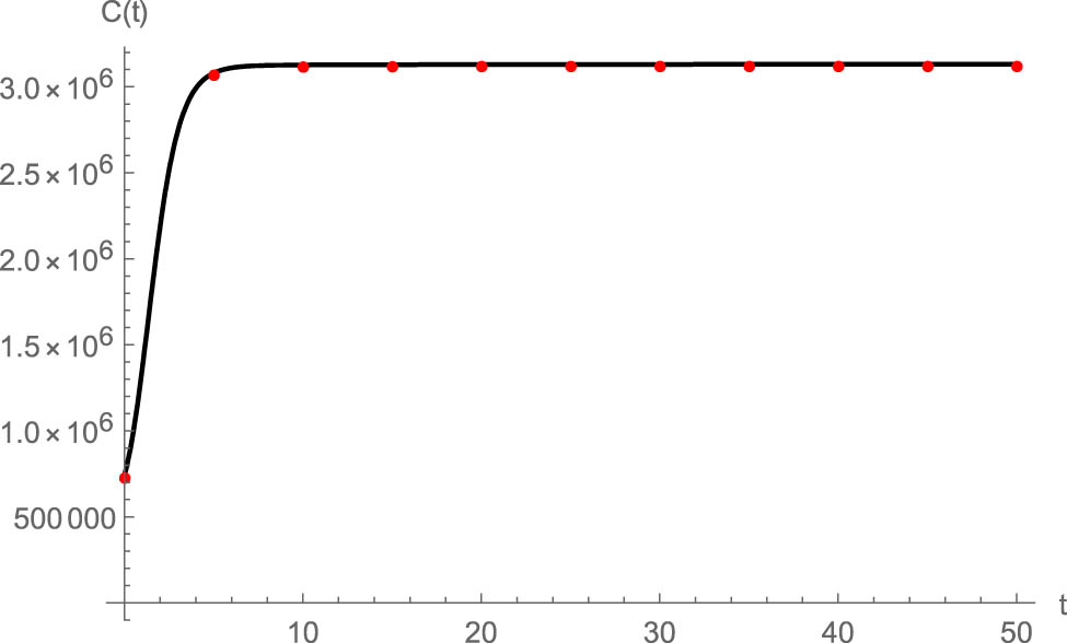
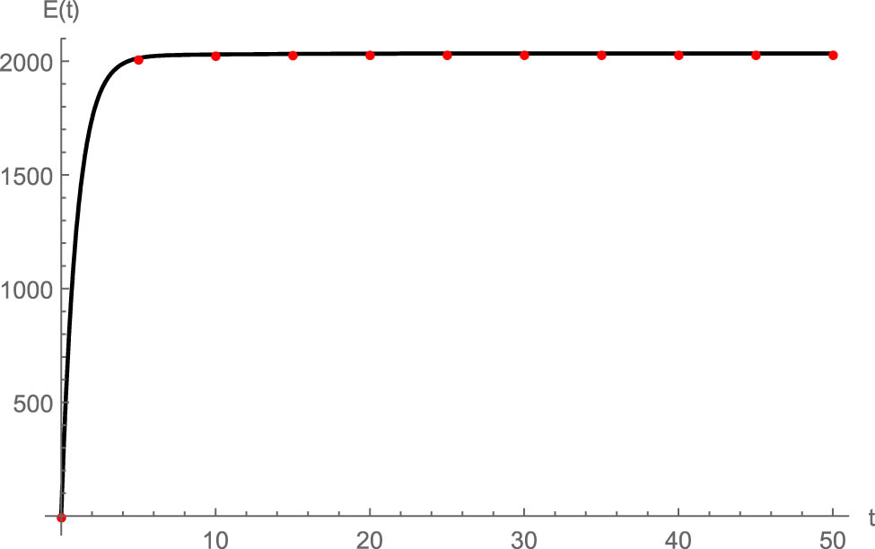
Since this problem cannot be solved exactly, there is no absolute and definite criterion to ensure the level of accuracy. However, comparing the results of the HZBW method with a numerical method, e.g., RK4, may relatively verify the obtained results. In this section, the proposed solution procedure is verified by comparing the results of the problem with integer-order derivatives (
Figures 1–5 depict the results of HZBW and RK4 methods. It is evident that these solutions are in great agreement, proving the trustworthiness of the HZBW method. To provide a more precise view of these results, they are listed in Table 7. It can be deduced that the results of these two methods are closely approximated as


Comparison of the results obtained by HZBW and RK4
|
|
|
|
|
|
|
||
|---|---|---|---|---|---|---|---|
|
|
HZBW |
|
|
|
|
|
|
| RK4 |
|
|
|
|
|
|
|
|
|
HZBW |
|
|
|
|
|
|
| RK4 |
|
|
|
|
|
|
|
|
|
HZBW |
|
|
|
|
|
|
| RK4 |
|
|
|
|
|
|
|
|
|
HZBW |
|
|
|
|
|
|
| RK4 |
|
|
|
|
|
|
|
|
|
HZBW |
|
|
|
|
|
|
| RK4 |
|
|
|
|
|
|
7.3 Computational cost
The computational cost of numerical methods for solving algebraic equations can be generally estimated analytically by calculating the number of algebraic operations. For those methods, e.g., the HZBW scheme, in which the focus is only on converting differential equations into algebraic equations, computational cost can be analysed by measuring CPU running time.
The CPU running time depends upon the programming language, hardware configuration, and the algorithms used in the computer code. Thus, comparing CPU running time between two different methods requires these factors to be the same for both methods. In this section, CPU running time for solving the problem with fractional derivatives for various values of
CPU running time in seconds for various sets of
|
|
|
|
|
|
|---|---|---|---|---|
|
|
|
|
|
|
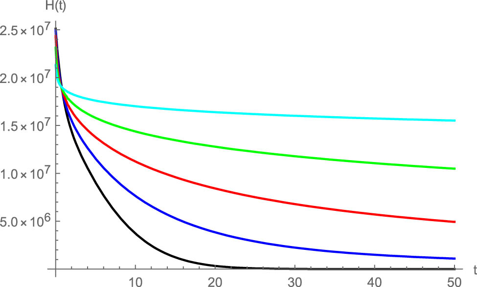
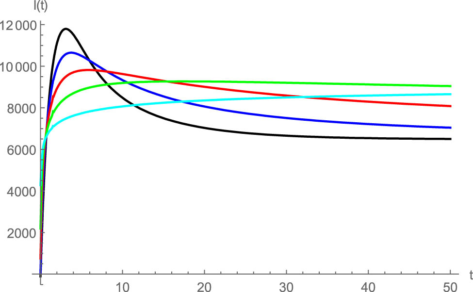
7.4 The effects of fractional orders
Since fractional derivatives are used to model the memory of a biological system, proper values for the fractional orders should be determined. In this section, the responses of the system to various values of the fractional orders are investigated for the case:
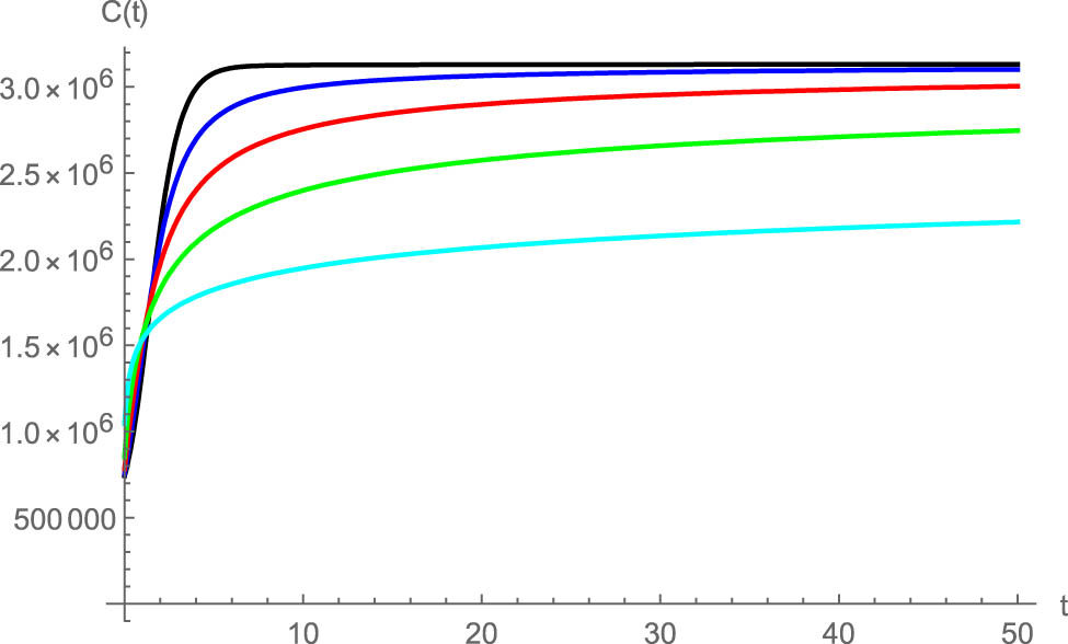
The effect of fractional order on
The effect of fractional order on

The effect of fractional order on
The effect of fractional order on
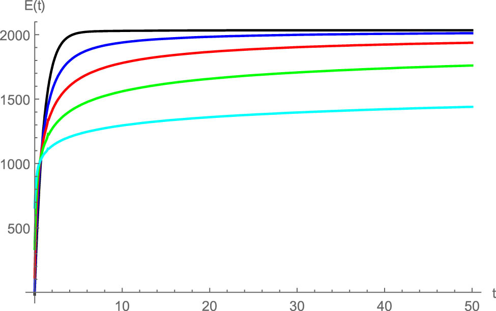
The effect of fractional order on
This study reveals that selecting proper values of fractional derivatives may significantly change the trend of breast cancer treatment.
8 Conclusion
In this article, non-orthogonal Zernike wavelets were introduced based on Zernike polynomials. Since these polynomials have demonstrated their superiority over similar functions and capability in accurate approximations, they were utilized to construct novel wavelets in this research. Besides, a new hybrid method based on combining these wavelets with block pulse functions was proposed to solve nonlinear fractional differential equations. The limitation of the presented Zernike wavelets was that they were not orthogonal. Although this issue was resolved by combining them with block pulse functions, creating orthogonal Zernike wavelets might be the objective of future works.
Moreover, this technique was employed to investigate a fractional model of breast cancer treatment. Error analysis was also conducted. Furthermore, convergence analysis, verification, and computational cost of the results were provided. Finally, the effects of fractional orders on the population of healthy, cancer stem, tumour, and immune cells, as well as the excess estrogen, were studied. It was demonstrated that this method is a promising technique for obtaining an accurate solution of nonlinear fractional differential equations. Moreover, it was illustrated that considering appropriate values of fractional derivatives may remarkably affect the trend of breast cancer treatment.
-
Funding information: The authors state no funding involved.
-
Author contributions: All authors equally contributed to this article and read and approved the final manuscript.
-
Conflict of interest: The authors declare that they have no conflicts of interest.
-
Data availability statement: All data, generated or used during the study, is available within the article.
References
[1] Kisela T. Fractional differential equations and their applications [dissertation]. Brno: Brno University of Technology; 2008.Search in Google Scholar
[2] Hedayati M, Ezzati R, Noeiaghdam S. New procedures of a fractional order model of novel coronavirus (COVID-19) outbreak via wavelets method. Axioms. 2021;10(2):122.10.3390/axioms10020122Search in Google Scholar
[3] Solís-Pérez JE, Gómez-Aguilar JF, Atangana A. A fractional mathematical model of breast cancer competition model. Chaos Solitons Fractals. 2019;127:38–54.10.1016/j.chaos.2019.06.027Search in Google Scholar
[4] Hussain A, Baleanu D, Adeel M. Existence of solution and stability for the fractional order novel coronavirus (nCoV-2019) model. Adv Differ Equ. 2020;2020(1):1–9.10.1186/s13662-020-02845-0Search in Google Scholar PubMed PubMed Central
[5] Atangana A. Modelling the spread of COVID-19 with new fractal-fractional operators: Can the lockdown save mankind before vaccination? Chaos Solitons Fractals. 2020;136:109860.10.1016/j.chaos.2020.109860Search in Google Scholar PubMed PubMed Central
[6] Wang B-H, Wang Y-Y, Dai C-Q, Chen Y-X. Dynamical characteristic of analytical fractional solitons for the space-time fractional Fokas-Lenells equation. Alex Eng J. 2020;59(6):4699–707.10.1016/j.aej.2020.08.027Search in Google Scholar
[7] Yu L-J, Wu G-Z, Wang Y-Y, Chen Y-X. Traveling wave solutions constructed by Mittag–Leffler function of a (2 + 1)-dimensional space-time fractional NLS equation. Results Phys. 2020;17:103156.10.1016/j.rinp.2020.103156Search in Google Scholar
[8] Fang J-J, Mou D-S, Wang Y-Y, Zhang H-C, Dai C-Q, Chen Y-X. Soliton dynamics based on exact solutions of conformable fractional discrete complex cubic Ginzburg–Landau equation. Results Phys. 2021;20:103710.10.1016/j.rinp.2020.103710Search in Google Scholar
[9] Wang B-H, Wang Y-Y. Fractional white noise functional soliton solutions of a wick-type stochastic fractional NLSE. Appl Math Lett. 2020;110:106583.10.1016/j.aml.2020.106583Search in Google Scholar
[10] Noeiaghdam S. A novel technique to solve the modified epidemiological model of computer viruses. SeMA J. 2019;76(1):97–108.10.1007/s40324-018-0163-3Search in Google Scholar
[11] Noeiaghdam S, Micula S. Dynamical strategy to control the accuracy of the nonlinear bio-mathematical model of malaria infection. Mathematics. 2021;9(9):1031.10.3390/math9091031Search in Google Scholar
[12] Noeiaghdam S, Suleman M, Budak H. Solving a modified nonlinear epidemiological model of computer viruses by homotopy analysis method. Math Sci. 2018;12(3):211–22.10.1007/s40096-018-0261-5Search in Google Scholar
[13] Bitsouni V, Tsilidis V. Mathematical modeling of tumor-immune system interactions: the effect of rituximab on breast cancer immune response. J Theor Biol. 2022;539:111001.10.1016/j.jtbi.2021.111001Search in Google Scholar PubMed
[14] Marino G, De Bonis MV, Lagonigro L, La Torre G, Prudente A, Sgambato A, et al. Towards a decisional support system in breast cancer surgery based on mass transfer modeling. Int Commun Heat Mass Transf. 2021;129:105733.10.1016/j.icheatmasstransfer.2021.105733Search in Google Scholar
[15] Nave O, Elbaz M. Artificial immune system features added to breast cancer clinical data for machine learning (ML) applications. Biosystems. 2021;202:104341.10.1016/j.biosystems.2020.104341Search in Google Scholar PubMed
[16] Jarrett AM, Hormuth DA, Wu C, Kazerouni AS, Ekrut DA, Virostko J, et al. Evaluating patient-specific neoadjuvant regimens for breast cancer via a mathematical model constrained by quantitative magnetic resonance imaging data. Neoplasia. 2020;22(12):820–30.10.1016/j.neo.2020.10.011Search in Google Scholar PubMed PubMed Central
[17] Simmons A, Burrage PM, Nicolau DV, Lakhani SR, Burrage K. Environmental factors in breast cancer invasion: a mathematical modelling review. Pathology. 2017;49(2):172–80.10.1016/j.pathol.2016.11.004Search in Google Scholar PubMed
[18] Abdelsalam SI, Zaher AZ. On behavioral response of ciliated cervical canal on the development of electroosmotic forces in spermatic fluid. Math Model Nat Phenom. 2022;17:27.10.1051/mmnp/2022030Search in Google Scholar
[19] Bhatti MM, Abdelsalam SI. Scientific Breakdown of a Ferromagnetic Nanofluid in Hemodynamics: Enhanced Therapeutic Approach. Math Model Nat Phenom. 2022;17.10.1051/mmnp/2022045Search in Google Scholar
[20] Abdelsalam SI, Bhatti MM. Unraveling the nature of nano-diamonds and silica in a catheterized tapered artery: highlights into hydrophilic traits. Sci Rep. 2023;13(1):5684.10.1038/s41598-023-32604-6Search in Google Scholar PubMed PubMed Central
[21] Raza R, Naz R, Abdelsalam SI. Microorganisms swimming through radiative Sutterby nanofluid over stretchable cylinder: Hydrodynamic effect. Numer Methods Partial Differ Equ. 2023;39(2):975–94.10.1002/num.22913Search in Google Scholar
[22] Tahmasbi A, Saki F, Shokouhi SB. Classification of benign and malignant masses based on Zernike moments. Comput Biol Med. 2011;41(8):726–35.10.1016/j.compbiomed.2011.06.009Search in Google Scholar PubMed
[23] Rdzanek WP. Sound radiation of a vibrating elastically supported circular plate embedded into a flat screen revisited using the Zernike circle polynomials. J Sound Vib. 2018;434:92–125.10.1016/j.jsv.2018.07.035Search in Google Scholar
[24] Yi M, Huang J. Wavelet operational matrix method for solving fractional differential equations with variable coefficients. Appl Math Comput. 2014;230:383–94.10.1016/j.amc.2013.06.102Search in Google Scholar
[25] Yi M, Wang L, Huang J. Legendre wavelets method for the numerical solution of fractional integro-differential equations with weakly singular kernel. Appl Math Model. 2016;40(4):3422–37.10.1016/j.apm.2015.10.009Search in Google Scholar
[26] Razzaghi M, Yousefi S. Sine-cosine wavelets operational matrix of integration and its applications in the calculus of variations. Int J Syst Sci. 2002;33(10):805–10.10.1080/00207720210161768Search in Google Scholar
[27] Kilicman A, Al Zhour ZAA. Kronecker operational matrices for fractional calculus and some applications. Appl Math Comput. 2007;187(1):250–65.10.1016/j.amc.2006.08.122Search in Google Scholar
[28] Ebadi MA, Hashemizadeh E. A new approach based on the Zernike radial polynomials for numerical solution of the fractional diffusion-wave and fractional Klein-Gordon equations. Phys Scr. 2018;93:125202.10.1088/1402-4896/aae726Search in Google Scholar
[29] Gasca M, Sauer T. On the history of multivariate polynomial interpolation. J Comput Appl Mathematics. 2000;122(1):23–35.10.1016/S0377-0427(00)00353-8Search in Google Scholar
[30] Yi M, Huang J, Wei J. Block pulse operational matrix method for solving fractional partial differential equation. Appl Math Comput. 2013;221:121–31.10.1016/j.amc.2013.06.016Search in Google Scholar
[31] Abernathy K, Abernathy Z, Baxter A, Stevens M. Global dynamics of a breast cancer competition model. Differ Equ Dyn Syst. 2020;28(4):791–805.10.1007/s12591-017-0346-xSearch in Google Scholar PubMed PubMed Central
© 2024 the author(s), published by De Gruyter
This work is licensed under the Creative Commons Attribution 4.0 International License.
Articles in the same Issue
- Editorial
- Focus on NLENG 2023 Volume 12 Issue 1
- Research Articles
- Seismic vulnerability signal analysis of low tower cable-stayed bridges method based on convolutional attention network
- Robust passivity-based nonlinear controller design for bilateral teleoperation system under variable time delay and variable load disturbance
- A physically consistent AI-based SPH emulator for computational fluid dynamics
- Asymmetrical novel hyperchaotic system with two exponential functions and an application to image encryption
- A novel framework for effective structural vulnerability assessment of tubular structures using machine learning algorithms (GA and ANN) for hybrid simulations
- Flow and irreversible mechanism of pure and hybridized non-Newtonian nanofluids through elastic surfaces with melting effects
- Stability analysis of the corruption dynamics under fractional-order interventions
- Solutions of certain initial-boundary value problems via a new extended Laplace transform
- Numerical solution of two-dimensional fractional differential equations using Laplace transform with residual power series method
- Fractional-order lead networks to avoid limit cycle in control loops with dead zone and plant servo system
- Modeling anomalous transport in fractal porous media: A study of fractional diffusion PDEs using numerical method
- Analysis of nonlinear dynamics of RC slabs under blast loads: A hybrid machine learning approach
- On theoretical and numerical analysis of fractal--fractional non-linear hybrid differential equations
- Traveling wave solutions, numerical solutions, and stability analysis of the (2+1) conformal time-fractional generalized q-deformed sinh-Gordon equation
- Influence of damage on large displacement buckling analysis of beams
- Approximate numerical procedures for the Navier–Stokes system through the generalized method of lines
- Mathematical analysis of a combustible viscoelastic material in a cylindrical channel taking into account induced electric field: A spectral approach
- A new operational matrix method to solve nonlinear fractional differential equations
- New solutions for the generalized q-deformed wave equation with q-translation symmetry
- Optimize the corrosion behaviour and mechanical properties of AISI 316 stainless steel under heat treatment and previous cold working
- Soliton dynamics of the KdV–mKdV equation using three distinct exact methods in nonlinear phenomena
- Investigation of the lubrication performance of a marine diesel engine crankshaft using a thermo-electrohydrodynamic model
- Modeling credit risk with mixed fractional Brownian motion: An application to barrier options
- Method of feature extraction of abnormal communication signal in network based on nonlinear technology
- An innovative binocular vision-based method for displacement measurement in membrane structures
- An analysis of exponential kernel fractional difference operator for delta positivity
- Novel analytic solutions of strain wave model in micro-structured solids
- Conditions for the existence of soliton solutions: An analysis of coefficients in the generalized Wu–Zhang system and generalized Sawada–Kotera model
- Scale-3 Haar wavelet-based method of fractal-fractional differential equations with power law kernel and exponential decay kernel
- Non-linear influences of track dynamic irregularities on vertical levelling loss of heavy-haul railway track geometry under cyclic loadings
- Fast analysis approach for instability problems of thin shells utilizing ANNs and a Bayesian regularization back-propagation algorithm
- Validity and error analysis of calculating matrix exponential function and vector product
- Optimizing execution time and cost while scheduling scientific workflow in edge data center with fault tolerance awareness
- Estimating the dynamics of the drinking epidemic model with control interventions: A sensitivity analysis
- Online and offline physical education quality assessment based on mobile edge computing
- Discovering optical solutions to a nonlinear Schrödinger equation and its bifurcation and chaos analysis
- New convolved Fibonacci collocation procedure for the Fitzhugh–Nagumo non-linear equation
- Study of weakly nonlinear double-diffusive magneto-convection with throughflow under concentration modulation
- Variable sampling time discrete sliding mode control for a flapping wing micro air vehicle using flapping frequency as the control input
- Error analysis of arbitrarily high-order stepping schemes for fractional integro-differential equations with weakly singular kernels
- Solitary and periodic pattern solutions for time-fractional generalized nonlinear Schrödinger equation
- An unconditionally stable numerical scheme for solving nonlinear Fisher equation
- Effect of modulated boundary on heat and mass transport of Walter-B viscoelastic fluid saturated in porous medium
- Analysis of heat mass transfer in a squeezed Carreau nanofluid flow due to a sensor surface with variable thermal conductivity
- Navigating waves: Advancing ocean dynamics through the nonlinear Schrödinger equation
- Experimental and numerical investigations into torsional-flexural behaviours of railway composite sleepers and bearers
- Novel dynamics of the fractional KFG equation through the unified and unified solver schemes with stability and multistability analysis
- Analysis of the magnetohydrodynamic effects on non-Newtonian fluid flow in an inclined non-uniform channel under long-wavelength, low-Reynolds number conditions
- Convergence analysis of non-matching finite elements for a linear monotone additive Schwarz scheme for semi-linear elliptic problems
- Global well-posedness and exponential decay estimates for semilinear Newell–Whitehead–Segel equation
- Petrov-Galerkin method for small deflections in fourth-order beam equations in civil engineering
- Solution of third-order nonlinear integro-differential equations with parallel computing for intelligent IoT and wireless networks using the Haar wavelet method
- Mathematical modeling and computational analysis of hepatitis B virus transmission using the higher-order Galerkin scheme
- Mathematical model based on nonlinear differential equations and its control algorithm
- Bifurcation and chaos: Unraveling soliton solutions in a couple fractional-order nonlinear evolution equation
- Space–time variable-order carbon nanotube model using modified Atangana–Baleanu–Caputo derivative
- Minimal universal laser network model: Synchronization, extreme events, and multistability
- Valuation of forward start option with mean reverting stock model for uncertain markets
- Geometric nonlinear analysis based on the generalized displacement control method and orthogonal iteration
- Fuzzy neural network with backpropagation for fuzzy quadratic programming problems and portfolio optimization problems
- B-spline curve theory: An overview and applications in real life
- Nonlinearity modeling for online estimation of industrial cooling fan speed subject to model uncertainties and state-dependent measurement noise
- Quantitative analysis and modeling of ride sharing behavior based on internet of vehicles
- Review Article
- Bond performance of recycled coarse aggregate concrete with rebar under freeze–thaw environment: A review
- Retraction
- Retraction of “Convolutional neural network for UAV image processing and navigation in tree plantations based on deep learning”
- Special Issue: Dynamic Engineering and Control Methods for the Nonlinear Systems - Part II
- Improved nonlinear model predictive control with inequality constraints using particle filtering for nonlinear and highly coupled dynamical systems
- Anti-control of Hopf bifurcation for a chaotic system
- Special Issue: Decision and Control in Nonlinear Systems - Part I
- Addressing target loss and actuator saturation in visual servoing of multirotors: A nonrecursive augmented dynamics control approach
- Collaborative control of multi-manipulator systems in intelligent manufacturing based on event-triggered and adaptive strategy
- Greenhouse monitoring system integrating NB-IOT technology and a cloud service framework
- Special Issue: Unleashing the Power of AI and ML in Dynamical System Research
- Computational analysis of the Covid-19 model using the continuous Galerkin–Petrov scheme
- Special Issue: Nonlinear Analysis and Design of Communication Networks for IoT Applications - Part I
- Research on the role of multi-sensor system information fusion in improving hardware control accuracy of intelligent system
- Advanced integration of IoT and AI algorithms for comprehensive smart meter data analysis in smart grids