Estimating the dynamics of the drinking epidemic model with control interventions: A sensitivity analysis
-
Yasir Nadeem Anjam
 and
Muhammad Farman
and
Muhammad Farman

Abstract
This article presents a non-linear mathematical model that captures the dynamics of drinking prevalence within a population. The model is analyzed under an optimal control framework, dividing the total population into four compartments: susceptible, heavy drinker, drinker in treatment, and recovered classes. The model’s validity is affirmed through considerations of positivity, boundedness, reproduction number, stability, and sensitivity analysis. Stability theory is employed to explore both local and global stabilities. Sensitivity analysis identifies parameters with a significant impact on the reproduction number (
1 Introduction
The ever-evolving research literature nominates the association of several physical, psychological, and socio-economic issues with the access use of alcohol. For example, Lees et al. [1] provided an enlightened account documenting the linkages of excessive alcohol and brain functioning ranging from compromised decision-making to memory loss. Similarly, World Health Organization [2,3] endorsed an intriguing association between chronic alcohol use and the development of medical complications, including a higher risk of liver disease, increased odds of cardiovascular issues, heart problems, high blood pressure, weakened immune system, and an increased risk of certain types of cancer. Furthermore, a thought-provoking investigation of Ferrari et al. [4] found vivid links connecting alcohol use with the streaming of negative emotions, such as depression, self-harm, suicidal attitude, anxiety, and alcohol dependence or addiction. Heavy drinking can also impair cognitive function, leading to difficulties with memory, attention, and decision-making. The main factors of alcohol drinking include income levels, education, employment status, and social norms. Research has found that individuals with lower incomes and lower levels of education are more likely to engage in heavy drinking [5]. Unemployment and job instability have also been associated with increased alcohol consumption [6]. Social norms and peer pressure can also influence drinking behaviors, as alcohol consumption is often seen as a way to fit in or cope with stress. The negative impulses of alcohol consumption are known to have drastic effects on more fragile groups of society, i.e., children. Excess drinking in mothers during pregnancy is found to be related to fetal alcohol spectrum disorders in children. Moreover, in a wider perspective, WHO Global Status Report [7] reported an astonishing estimate of 30% of absenteeism associated with alcohol, in Costa Rica. However, in the UK, the share of alcohol usage in fatal accidents is found to be 60%. The degree of burden of alcohol consumption on the health care systems can be witnessed from the documentation of Johnson et al. [8] reporting a 47% increase in the rate of all alcohol-related emergency visits from 2006 to 2014. From a global perspective, the unchecked use of alcohol is found to be related to the instigation of more than 200 medical complexities, including liver cirrhosis, malignancies, and cardiovascular disease [9,10]. The resulting number of deaths is counted as higher as 3.3 million fatalities per annum, contributing to a notable share of 6% of all deaths, globally [3]. More alarmingly, excessive alcohol consumption is becoming an emerging trend in adolescents aged 15–19 years [11]. Almost 46% of the world’s adolescents aged 15–19 years reported having overused alcohol. In 2016, the National Survey on Drug Use and Health reported that 85.6% of people aged 18 and older drank alcohol, in the USA.
Dynamic modeling, employing mathematical frameworks such as differential equations, unveils the temporal evolution of systems, articulating variable interactions for precise predictions and analysis across diverse fields. Mathematical representations unravel patterns, identify parameters, and enhance our understanding of complex systems. The impact of dynamic modeling spans scientific progress and technological innovations, underscoring its significance across disciplines [12]. Chen has made significant contributions to dynamic modeling, particularly in integrated energy systems and natural gas dynamics [13]. His work involves developing robust state estimators and Kalman filter-based approaches to enhance the accuracy and reliability of state predictions [14]. Focusing on complex energy networks and pipeline systems, Chen’s research addresses critical challenges and offers insights for advancing dynamic modeling methodologies in the energy sector.
Mathematical studies serve as invaluable tools for evaluating, testing, and implementing strategies on both short- and long-term scales, particularly in addressing chronic relapsing diseases such as alcoholism. There has been limited research on mathematical modeling methods for social problems such as alcohol and drug use, despite these issues often being referred to as epidemics, in contrast to research on other epidemic problems. However, in recent years, an increasing number of mathematicians have dedicated their efforts to developing mathematical models aimed at understanding and addressing alcohol-related concerns. Khan and Khan [15] proposed a mathematical model for drinking using numerical analysis of fractional order. Chinnadurai et al. [16] focused on employing mathematical modeling to analyze strategies for controlling alcohol consumption, particularly examining their impact on socioeconomically disadvantaged populations. Through the optimal control approach, Imken and Fatmi [17] introduced a novel mathematical model to investigate alcohol consumption within the diabetic population, especially under antidiabetic drug treatments. ur Rahman et al. [18] proposed a fractional mathematical model for drinking under Atangana–Baleanu Caputo derivatives. Bunonyo et al. [19] research focused on using the eigenvalue method to develop a mathematical model for the time-dependent concentration of alcohol in the human bloodstream, contributing to a deeper understanding of alcohol metabolism dynamics and potentially informing strategies for alcohol-related risk assessment and management. Huo and Wang’s nonlinear mathematical model [20] illustrated the impact of awareness campaigns on binge drinking, demonstrating their effectiveness in mitigating alcohol-related issues. Ma et al. [21] tested a mathematical model of alcoholism as a communicable disease, incorporating awareness campaigns and a time delay, using optimal control techniques. Wang et al. [22] proposed and investigated a nonlinear model of alcoholism with optimal control to prevent interactions between susceptible and infected individuals. Sharma et al. [23] established a mathematical model of alcohol consumption, examining the stability and existence of an endemic equilibrium without drinking, and analyzing the sensitivity of
In recent times, there has been a growing emphasis on employing optimal control strategies to improve viral transmission management. These applications extend beyond medical contexts and encompass various areas such as policy development, engineering risk assessment, emergency preparedness, and control program refinement [30,31]. Optimal control strategies are designed to identify effective protocols for addressing complex problems, utilizing mathematical techniques such as dynamic programming, Pontryagin’s principle, or model predictive control [32]. Utilizing optimal control techniques in mathematical models offers benefits by enabling the identification of efficient control strategies to achieve desired outcomes, including improved system performance, maximized benefits, or reduced costs [33]. Verma et al. proposed a mathematical model to investigate coronavirus dynamics, considering the impact of lockdown as an epidemiological measure [34]. They also studied a nonlinear smoking model to analyze interactions between smokers and smoking quitters [35]. Moreover, optimal control strategies have been introduced for coronavirus disease 2019, human immunodeficiency virus, and Dengue through mathematical models that capture relationships among these infectious diseases [36]. For further insights, references such as Omame et al. [37] sightsee backward bifurcation and optimal control in a co-infection model for severe acute respiratory syndrome coronavirus 2 (SARS-CoV-2) and zika virus, while Omame et al. [38] delve into SARS-CoV-2 and HBV co-dynamics modeling.
Motivated by the importance of the aforementioned issue, this study delves into the application of optimal control theory to devise a new mathematical framework capable of illustrating drinking prevalence trends in a community. The goal of the optimal control scheme is to establish feasible control laws that optimize specific performance metrics. This article introduces a proposed mathematical model for a drinking epidemic, categorizing the entire population into four classes: susceptible drinkers, individuals in treatment, heavy drinkers, and recovered drinkers. Initially, we validate the proposed model by examining fundamental properties such as boundedness, positivity, reproduction number, equilibrium points, stability, and conducting sensitivity analyses. We conduct comprehensive stability analyses at equilibrium points to assess both local and global stabilities, outlining the legitimacy of the model through detailed sensitivity analysis and documenting local and global features. Subsequently, we develop the drinking epidemic model using control variables derived from qualitative optimal control principles, aiming to maximize susceptible and recovered drinkers while minimizing heavy drinkers and optimizing the aforementioned compartments. The optimal control involves two control variables: a social awareness campaign
This article is organized into the following sections. Section 2 concentrates on model analysis, while Section 3 delves into sensitivity analysis. Section 4 discusses the stability aspects of the model under consideration. Section 5 elaborates on the integration of optimal control, emphasizing the implementation of more effective health interventions. Finally, Section 6 summarizes the key findings of this study.
1.1 Model formulation
Understanding the transmission patterns of diseases and creating effective control strategies heavily relies on mathematical models. Therefore, it is essential to focus on delineating the epidemiological facets of the disease and pinpointing crucial, adjustable parameters to bolster disease control measures.
This study delves into exploring a mathematical model aimed at understanding the drinking epidemic within the human population [40]. It highlights several key limitations in the model analysis, including simplification of real-world complexities, potential oversights in parameter selection, reliance on assumed relationships, and the absence of dynamic external factors. These constraints may limit the model’s ability to fully capture the complexities of human behavior and societal dynamics, potentially impacting the generalizability of the findings. Therefore, caution is advised in interpreting the predictions, as real-world applicability may be constrained by the inherent simplifications in the modeling approach. Additionally, certain assumptions were made in developing the proposed drinking epidemic model. The epidemic occurs within a closed environment, where factors such as sex, race, and social status do not influence the likelihood of developing heavy drinking habits. Members interact homogeneously, meaning they have an equal degree of interaction with one another. Heavy drinking behavior can be transmitted to non-drinkers when they come into contact with individuals who regularly consume large amounts of alcohol. Individuals undergoing treatment for their drinking habits may transition through stages of recovery and susceptibility, potentially leading to a return to heavy drinking. Conversely, those who have successfully stopped drinking enter the recovery compartment.
At any time
Therefore, the model classes include the susceptible compartment
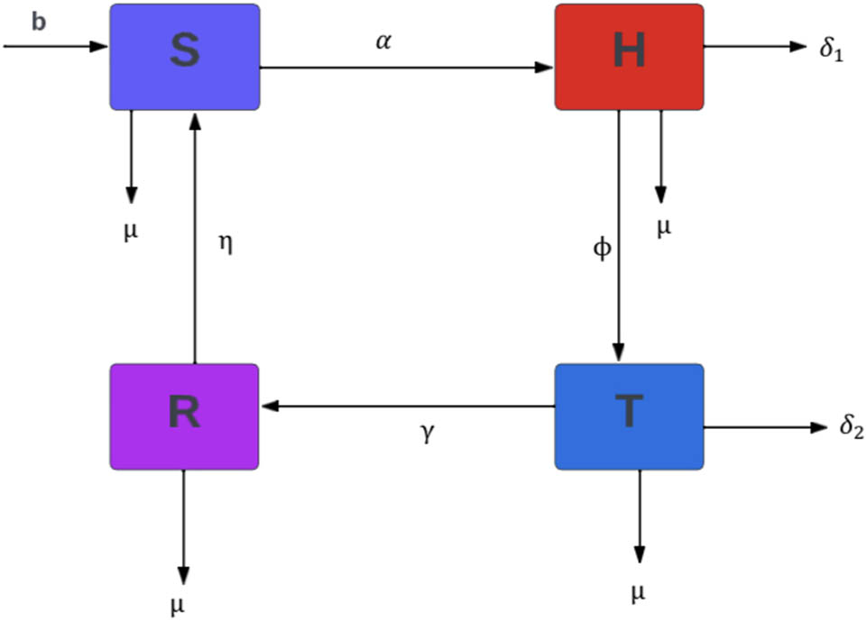
The schematic diagram elucidates the dynamics of transmission in drinking behavior.
Hence, the total population at any given time
Therefore, the fundamental model for the drinking epidemic is governed by a system of nonlinear differential equations, which include:
subject to the initial conditions,
The specifics of each term that impact the system, as outlined in Model (1), are identified in Table 1.
Explanation for each term in the equations of Model (1) is presented
| Terms of each equation | Explanation |
|---|---|
|
|
Recruitment rate of the susceptible people |
|
|
The rate of transmission from the susceptible class to individuals with heavy drinking habits |
|
|
Transmission rate of recovered people |
|
|
The rate of natural mortality among individuals in the susceptible population. |
|
|
The mortality rate caused by drinking among individuals in the heavy drinker population |
|
|
Proportion of drinking people of heavy drinker class |
|
|
The mortality rate attributed to drinking among individuals in the drinker in treatment population |
|
|
Recovered rate of drinker in treatment people |
|
|
Mortality rate among heavy drinkers |
|
|
Natural death rate of drinker in treatment people |
|
|
Natural death rate of recovered people |
2 Qualitative analysis of the proposed model
In the forthcoming section, our analysis will focus on the mathematical formulation encapsulated in Model (1). Our examination will delve into the aspects of boundedness and positivity within the model. Additionally, we will determine the equilibrium points and compute the basic reproduction number.
2.1 Positivity
Positivity constraints are imposed on both the initial conditions and parameters in the devised model, ensuring that their values remain non-negative or greater than zero throughout the modeling process. This imposition enhances the model’s reliability by minimizing the occurrence of unrealistic outcomes, thereby improving its applicability and making it more representative of real-world scenarios and behaviors. Consequently, we rearrange Model (1) in accordance with these constraints.
where
In a stress-free scenario,
2.2 Boundedness
Boundedness in the drinking model refers to inherent constraints within the study, such as the exclusive focus on specific demographics or contexts. These limitations risk compromising the model’s reliability by narrowing its perspective and potentially overlooking broader behavioral patterns. As a result, reduced generalizability restricts the model’s applicability to specific circumstances and populations, which may compromise its ability to capture the nuanced complexity of real-world drinking behaviors. To understand the aforementioned model, we need the bounds on the dependent variables involved. To achieve this, we must determine the feasible region of attraction as outlined in the following theorem.
Theorem 2.1
There is a positive
Proof
The solutions of System (1) are greater than zero, now in the first compartment of System (1) as
Thus,
where
Clearly,
2.3 Equilibrium points
Equilibrium points denote the stable-state prevalence of individuals engaged in drinking behavior, wherein the influx of new drinkers is counterbalanced by the rates of recoveries and mortality. There exist two equilibrium points: the drinking-free equilibrium point, and the drinking-present equilibrium point. For the computation of the drinking model, the process involves setting the left-hand side of Model (1) equations equal to zero.
2.3.1 Drinking-free equilibrium point (
E
0
)
In the modeling of drinking behaviors, a drinking-free equilibrium point (
2.3.2 Drinking endemic equilibrium point (
E
1
)
An endemic equilibrium point (
and
2.4 Reproduction number
The basic reproduction number
We utilize the next-generation matrix method [42,43] to calculate the reproduction number. The matrices
The Jacobian of
The basic reproduction number
Hence, the basic reproduction number
If
3 Sensitivity analysis
Sensitivity analysis plays a crucial role in assessing the impact of input parameters on the dynamics of the epidemic drinking model. The parameters selected for sensitivity analysis in this study align closely with the model’s objectives, which aim to understand the dynamics of drinking behavior and its transmission within a population. These carefully chosen parameters represent key factors influencing the spread of drinking behaviors, including the transmission rate of heavy drinkers, natural death rate, drinking-induced death rates, and the proportion of individuals entering treatment. The sensitivity indices used in the drinking model to calculate the reproduction number (
The sensitivity estimation for the reproduction number concerning various parameters is presented as follows:
Sensitivity analysis is commonly used to identify parameters significantly impacting the reproduction number
Indices of sensitivity and parameters affecting the reproduction number
| Parameters | Sensitivity indices |
|---|---|
|
|
+ |
|
|
|
|
|
|
|
|
|
A notable revelation from this sensitivity analysis is the substantial influence of the transmission rate of heavy drinkers on the reproduction number (
Parameters and its value of Model (1)
| Parameters | Description | Value | Sources |
|---|---|---|---|
|
|
Recruitment rate of the susceptible people | 0.25 | Estimated |
|
|
Transmission rate from susceptible class to heavy drinker people | 0.7 | [40] |
|
|
Transmission rate from recovered people to susceptible people | 0.1 | [40] |
|
|
Natural death rate | 0.25 | [45] |
|
|
Drinking-induced death rate of heavy drinker people | 0.35 | [45] |
|
|
Proportion of drinking entering of drinker in treatment class | 0.7 | [40] |
|
|
Drinking-induced death rate of drinker in treatment people | 0.3 | [45] |
|
|
Recovered rate of drinker in treatment people | 0.09 | [40] |
The effect of different significant model parameters on the value of
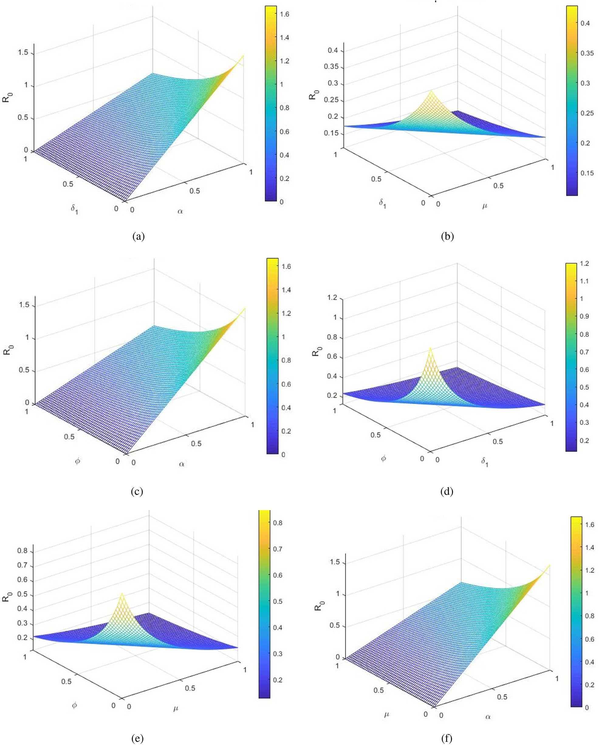
Fluctuation of different compartmental parameters and their effect on the basic reproduction number
4 Analysis of stability
In this segment, we explore the local stability and global stability of the developed model at equilibrium points. The local stability is assessed by analyzing the eigenvalues of the Jacobian matrix at the equilibrium point. An equilibrium point is deemed locally stable if all eigenvalues have negative real parts. Global stability entails studying the system’s behavior across its whole range, frequently necessitating progressive mathematical techniques such as Lyapunov analysis.
4.1 Local stability
A locally stable system tends to revert to its equilibrium state after experiencing minor disruptions, showcasing resilience and a tendency to maintain its original configuration near the equilibrium point. Conducting a local stability analysis within a drinking model aims to assess how minor disturbances can affect the persistence or reduction of drinking behavior. In the context of drinking models, the concept of local stability at equilibrium points becomes a crucial framework for understanding the complex dynamics of alcohol consumption and its spread within a population. In this discussion, we explore the locally stable drinking-free equilibrium point and the endemic equilibrium point in the devised model, utilizing the following theorem [29].
Theorem 4.1
The drinking-free equilibrium point
Proof
The Jacobian matrix of drinking-free equilibrium point
Evaluating the Jacobian matrix at the drinking-free equilibrium yields
The resulting eigenvalues are
Theorem 4.2
The endemic equilibrium point
Proof
The Jacobin matrix is computed as
where
Substituting
The auxiliary equation of (5) can be calculated as follows:
The aforementioned equation can be written as
where
Applying the Routh–Hurwitz criterion to fourth-order polynomials [46], we ensure that
4.2 Global stability
Global stability in a drinking model investigates whether, under various conditions, the system converges to a stable state regarding drinking behavior across its entire range. Global stability analysis in the drinking model is essential for understanding the sustained, long-term dynamics of population drinking behavior. By examining the system’s equilibrium conditions and considering the influence of broader societal factors, this analysis provides a comprehensive understanding of how the population’s drinking patterns evolve over an extended period. Such insights are crucial for developing enduring public health strategies and policies tailored to address persistent trends and dynamics in alcohol consumption within the population. Global stability analyses offer a holistic framework for effective long-term planning and management of drinking dynamics. In this discussion, we investigate the globally stable equilibrium points for both drinking-free and endemic states in the proposed model, employing the methodology outlined in the study by Anjam et al. [29].
Theorem 4.3
The drinking-free equilibrium point
Proof
The global stability of the devised model at point
Upon computing the time derivative of equation (8) and applying it to the system of equations in (1), the following result is obtained:
It is verifiable that
Theorem 4.4
The endemic equilibrium point
Proof
The global stability is established by formulating the Lyapunov function at the endemic equilibrium points
Upon calculating the time derivatives of the aforementioned equation and utilizing Model (1), the resulting expression is as follows:
As a consequence,
4.3 Results from numerical stability analysis
Runge–Kutta (RK) method is highly favored in epidemiological modeling because of its accuracy and robustness in solving the differential equations that govern disease dynamics. These models typically involve a system of coupled differential equations that describe interactions among different population compartments. The fourth-order RK method is particularly noteworthy for its high accuracy in approximating solutions to these equations, guaranteeing reliable and precise numerical results. Its robust convergence properties enhance both stability and efficiency, making it highly effective in solving diverse mathematical problems, especially those involving intricate and dynamic infectious disease dynamics. In this context, we employ the RK method to solve our proposed deterministic model, leveraging its ability to compute solutions through a series of approximations based on weighted function evaluations. Notably, the fourth-order RK method delivers accurate results with minimal model evaluations, making it a preferred choice for obtaining numerical solutions in Model (1). Hence, we obtain
To numerically solve the proposed model, we initially focus on the equation for the susceptible compartment
Similarly, the remaining compartments of the proposed model are solved, respectively, and give,
4.3.1 Algorithm
Step 1:
Step 2: for
Step 3: for
For the graphical depiction of the stability analysis, MATLAB software is utilized to run the aforementioned findings. The graphs presented in the figures below are generated using compartmental initial conditions for the devised model:
Figures 3, 4, 5, 6 depict the stability dynamics of all population classes under various initial conditions. The susceptible class varies in magnitude with values of 0.5, 0.35, 0.2, and 0.05, showing a direct relationship among the size of the susceptible population and the time required to achieve stability (Figure 3). Similarly, Figure 4 illustrates stability achievements across different sizes of the heavy drinker class, with values of 0.25, 0.20, 0.15, and 0.10. The heavy drinker population decreases over time, stabilizing after 10 days. The population in the drinkers in treatment class is shown for various prevalence levels, represented by values such as 0.15, 0.13, 0.11, and 0.09 in Figure 5. The number of individuals in treatment for drinking initially rises over time, followed by a rapid decline as time progresses. Figure 6 illustrates the correlation between stability and the varying extent of the recovered population, considering values such as 0.1, 0.09, 0.08, and 0.07. The population experiences an initial rapid decrease, stabilizing with constant numbers after 15 days.
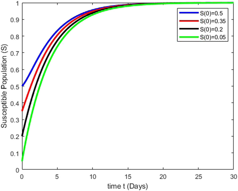
Simulation results illustrate how changes in the susceptible class
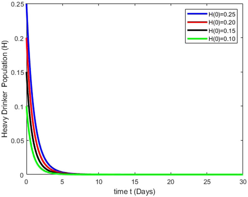
Simulation results depict how variations in the heavy drinker class
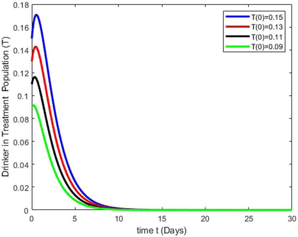
Simulation results depict how variations in the drinker in treatment class
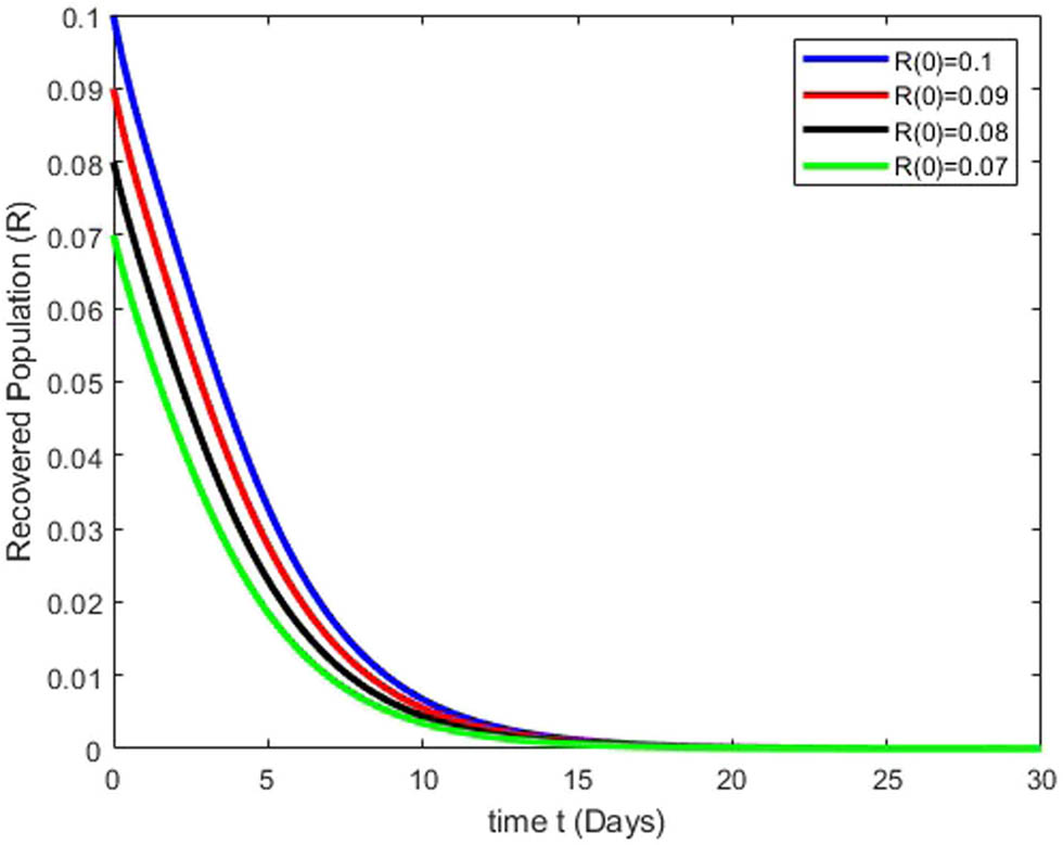
Simulation results illustrate how changes in the recovered class
5 Optimal control theory
This section delves into the application of the drinking model with regard to optimal control strategies. Optimal control is utilized to intercede in the transmission of drinking within a specific community. The integration of an optimal control strategy, focusing on awareness campaigns (
whereas the initial conditions are,
Therefore, we consider an optimal control problem, wherein the objective function is specified as
where
Here,
Furthermore, Pontryagin’s maximum principle [53,54] is used to find the optimal control strategy
Theorem 5.1
For the optimal control Problem (14), there exists a
Proof
A variety of techniques are considered to quantify the effectiveness of the control scheme [55,56], and consequently, nonnegative values are witnessed for control variables along with state variables. The convexity and the closeness of control variables describe the degree of solidity necessary to validate the control system. Moreover, it is noteworthy that the integrand exhibits a convex nature, representing an objective function in the form of
Moreover, the presence of non-trivial vector functions like
The outcomes are achieved by the employment of the required condition to the Hamiltonian function.□
5.1 Existence of the optimal control problem
In this section, we establish the existence of optimal control by ensuring that all conditions of the control system are met at the initial time
The minimum optimal control value is determined by formulating the Hamiltonian function
The resultant system, in terms of adjoint variable
Theorem 5.2
Given an optimal control
using the transversality criterion
Proof
Let us assume that
Theorem 5.3
The optimal control pair
Proof
The application of optimal conditions provided outcomes such as
The control variable is also solved such as
One may note that the condition of control space remains expressible as under
In simplification, the control variables are documented as follows:
The optimal system is now given as:
The state variable and control variable in the optimal formation are achieved by the employment of an adjoint variable, the optimal system along with the initial conditions. The positivity of the second-order derivative of the objective function with respect to control variables is obvious. Therefore, the resultant Hamiltonian is documented as
5.2 Computational simulation and discussion
In this section, we aim to validate the proposed control strategy through numerical evaluation. We enrich the strategic framework by integrating a wide range of parametric settings. The numerical analysis commences with initializing the compartmental initial conditions from the study by Adu et al. [40] for our proposed model, comprising
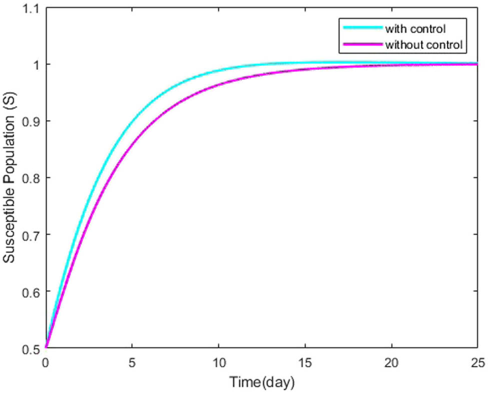
Dynamics behavior of susceptible individual
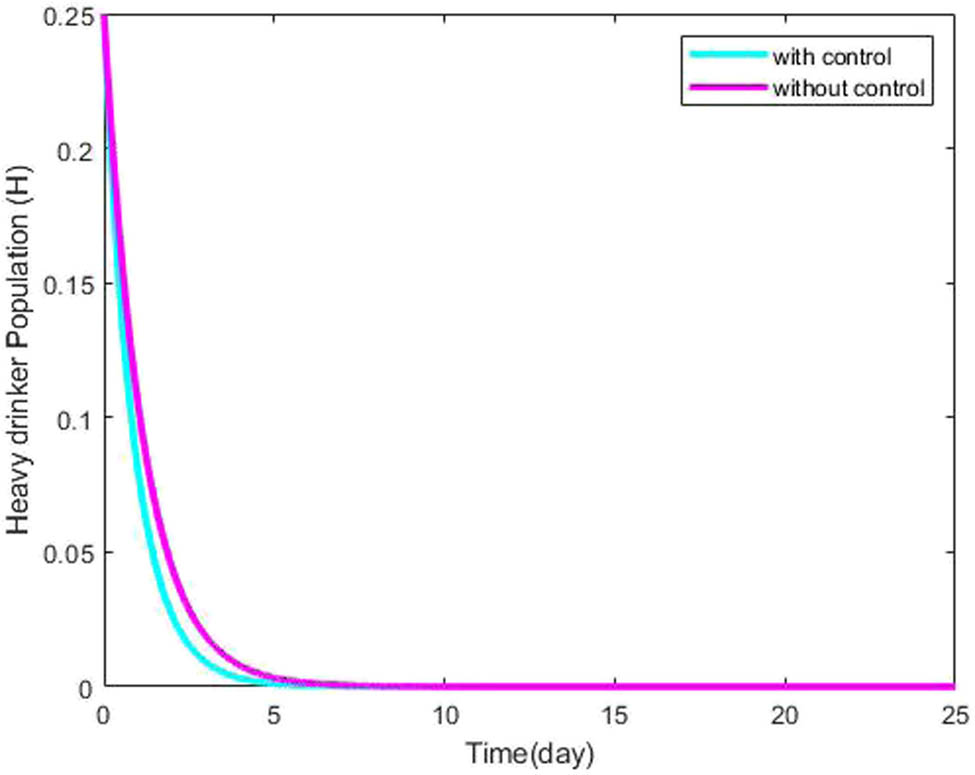
Dynamics behavior of heavy drinker individual
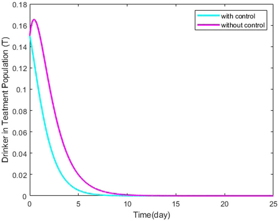
Dynamics behavior of drinker in treatment individual
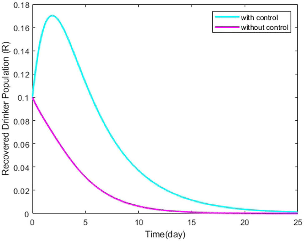
Dynamics behavior of recovered individual
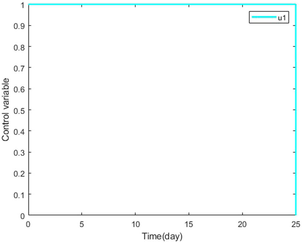
Dynamics of control variable
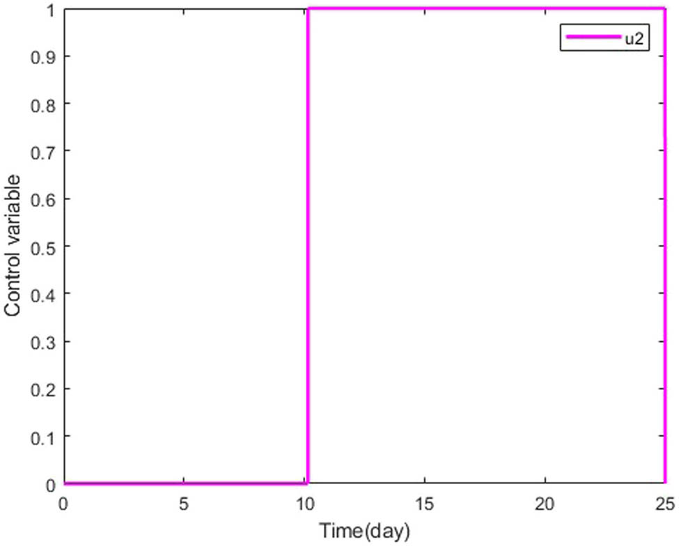
Dynamics of control variable
6 Conclusion
This study is related to the development of a novel deterministic mathematical model elaborating the dynamics of the drinking epidemic model under the launch of an optimal control scheme. The investigation focuses on stratifying the population into four compartments: the susceptible class, heavy drinker class, drinkers in treatment class, and recovered drinker class. To ensure generalizability, a wide range of parametric settings are employed, encompassing the recruitment rate of the susceptible class, transmission rates from the susceptible class to the heavy drinker class, and from the recovered class to the susceptible class, natural death rate, drinking-induced death rates in the heavy drinker and treatment classes, the proportion of individuals entering the treatment class, and recovery rate. Throughout the investigation, a comprehensive analysis is provided, covering aspects such as positivity, boundedness, equilibrium points, basic reproduction number, stability, and sensitivity. The model ensures boundedness and positivity by incorporating constraints and selecting appropriate functional forms. This precautionary approach prevents unrealistic growth of variables, aligning the model with real-world constraints and enhancing its reliability. The careful management of these aspects improves the model’s applicability, offering policymakers an accurate representation that supports well-informed decision-making within practical limitations. The analysis of stability in the model indicates that when
We initiate the optimal control process by integrating two time-dependent variables: a social awareness campaign and treatment, both acting as control variables. An optimal control problem is formulated by defining an objective function aimed at determining the optimal values for these control variables to minimize overall costs. By applying Pontryagin’s maximum principle, we derive significant conditions for the optimal solution. Our research investigates the viability of two different optimal control methodologies. Numerical simulations conducted using MATLAB validate the effectiveness of the proposed control strategies. Graphical results reveal that the simultaneous use of both control variables is more effective in reducing the transmission flow of drinking behavior. These findings are extensively discussed, considering scenarios with and without optimal control. Through rigorous analytical procedures, we establish the utility of the control strategy in achieving optimal conditions across all four compartments. The susceptible population is estimated to show a gradual increase with control implementation, while a notable decrease in the proportions of heavy drinkers and individuals in treatment is observed with optimal control. Additionally, the recovery rate is significantly faster with the use of optimal control. Furthermore, our research advocates that simulations incorporating time-dependent controls are supplementary cost-effective equated to those utilizing time-independent controls.
In future endeavors, extending the model to include fractional-order dynamics alongside optimal control remains an intriguing avenue. This approach is expected to provide deeper insights into the dynamics of drinking behavior in society by leveraging available information more effectively. Additionally, there will be a strong emphasis on assessing the proposed scheme’s applicability across diverse geographical regions, socio-economic strata, and varying healthcare access levels. Understanding how these strategies interact or counteract each other will help formulate more effective plans for disease control on a global scale. Moreover, future research may also focus on integrating real-time data and advanced machine-learning techniques to enhance the accuracy and predictive capabilities of the model.
-
Funding information: This research was supported by the Deanship of Research Development, Prince Mohammad Bin Fahd, University, Alkhubar 31952, Saudi Arabia.
-
Author contributions: All authors have accepted responsibility for the entire content of this manuscript and have approved its submission. YNA and KI designed the concept, while KI and SAC carried out the methodology. MF and SM developed the software model code and conducted the simulations. YNA, SM, and NS prepared the manuscript with contributions from all coauthors. The authors applied the SDC approach to determine the sequence of authors.
-
Conflict of interest: The authors declare that they have no known competing financial interests or personal relationships that could have appeared to influence the work reported in this article.
-
Data availability statement: Data sharing is not applicable to this article as no datasets were generated or analysed during the current study.
References
[1] Lees B, Meredith LR, Kirkland AE, Bryant BE, Squeglia LM. Effect of alcohol use on the adolescent brain and behavior. Pharmacol Biochem Behav. 2020;192:172906. 10.1016/j.pbb.2020.172906Search in Google Scholar PubMed PubMed Central
[2] World Health Organization. Global status report on alcohol and health; 2014. p. 1–68.Search in Google Scholar
[3] James LM, Van Kampen E, Miller RD, Engdahl BE. Risk and protective factors associated with symptoms of post-traumatic stress, depression, and alcohol misuse in OEF/OIF veterans. Military Med. 2013;178(2):159–65. 10.7205/MILMED-D-12-00282Search in Google Scholar PubMed
[4] Ferrari AJ, Charlson FJ, Norman RE, Patten SB, Freedman G, Murray CJ, et al. Burden of depressive disorders by country, sex, age, and year: findings from the global burden of disease study 2010. PLoS Med. 2013;10(11):1001547. 10.1371/journal.pmed.1001547Search in Google Scholar PubMed PubMed Central
[5] Keyes KM, Hasin DS. Socio-economic status and problem alcohol use: the positive relationship between income and the DSM-IV alcohol abuse diagnosis. Addiction. 2008;103(7):1120–30. 10.1111/j.1360-0443.2008.02218.xSearch in Google Scholar PubMed PubMed Central
[6] Catalano R, Dooley D, Wilson G, Hough R. Job loss and alcohol abuse: a test using data from the epidemiologic Catchment area project. J Health Soc Behav. 1993;34:215–25. 10.2307/2137203Search in Google Scholar
[7] WHO Global Status Report. Social Problems associated with alcohol use, Alcohol consumption and the workplace. 2004. p. 59–60.Search in Google Scholar
[8] Johnson RC, Schwitters SY, Wilson JR, Nagoshi CT, McClearn GE. A cross-ethnic comparison of reasons given for using alcohol, not using alcohol or ceasing to use alcohol. J Stud Alcohol. 1985;46(4):283–8. 10.15288/jsa.1985.46.283Search in Google Scholar PubMed
[9] World Health Organization. Global status report on alcohol and health 2018. World Health Organization; 2019. Search in Google Scholar
[10] Anderson P. The UK government’s alcohol strategy. Drugs Educat Prevent Policy. 2012;19(5):360–1. 10.3109/09687637.2012.698425Search in Google Scholar
[11] WHO global status report on alcohol and health Geneva. 2014.Search in Google Scholar
[12] Smith JC. Basic interdiction models. Wiley encyclopedia of operations research and management science. Hoboken: John Wiley and Sons; 2010. 10.1002/9780470400531.eorms0089Search in Google Scholar
[13] Chen L, Li Y, Huang M, Hui X, Gu S. Robust dynamic state estimator of integrated energy systems based on natural gas partial differential equations. IEEE Trans Industry Appl. 2022;58(3):3303–12. 10.1109/TIA.2022.3161607Search in Google Scholar
[14] Ma P, Yao N, Yang X. Service quality evaluation of terminal express delivery based on an integrated SERVQUAL-AHP-TOPSIS approach. Math Problems Eng. 2021;2021:1–10. 10.1155/2021/8883370Search in Google Scholar
[15] Khan FM, Khan ZU. Numerical analysis of fractional order drinking mathematical model. J Math Tech Model. 2024;1(1):11–24. Search in Google Scholar
[16] Chinnadurai K, Athithan S, Kareem MG. Mathematical modelling on alcohol consumption control and its effect on poor population. IAENG Int J Appl Math. 2024;54(1):1–9. Search in Google Scholar
[17] Imken I, Fatmi NI. A new mathematical model of drinking alcohol among diabetes population taking anti-diabetic drugs: an optimal control approach. Commun Math Biol Neurosci. 2024;2024:25. Search in Google Scholar
[18] ur Rahman M, Arfan M, Shah Z, Alzahrani E. Evolution of fractional mathematical model for drinking under Atangana-Baleanu Caputo derivatives. Phys Scr. 2021;96(11):115203. 10.1088/1402-4896/ac1218Search in Google Scholar
[19] Bunonyo KW, Ebiwareme L, Iworiso PB. Mathematical modeling of time-dependent concentration of alcohol in the human bloodstream using the eigenvalue method. TWIST. 2024;19(1):58–64. 10.37745/ijmss.13/vol11n4119Search in Google Scholar
[20] Huo HF, Wang Q. Modelling the influence of awareness programs by media on the drinking dynamics. Abstr Appl Anal. 2014;2014:1–8. 10.1155/2014/938080Search in Google Scholar
[21] Ma SH, Huo HF, Meng XY. Modelling alcoholism as a contagious disease: a mathematical model with awareness programs and time delay. Discrete Dynams Nature Soc. 2015;2015(2):1–13. 10.1155/2015/260195Search in Google Scholar
[22] Wang XY, Huo HF, Kong QK, Shi WX. Optimal control strategies in an alcoholism model. Abstr Appl Anal. 2014;2014:1–18. 10.1155/2014/954069Search in Google Scholar
[23] Sharma S, Samanta GP. Drinking as an epidemic: a mathematical model with dynamic behaviour. J Appl Math Inform. 2013;31(1–2):1–25. 10.14317/jami.2013.001Search in Google Scholar
[24] Michel AN, Hou L, Liu D. Stability of dynamical systems. Birkhaüser, Boston, MA. 2008. Search in Google Scholar
[25] Huo HF, Chen YL, Xiang H. Stability of a binge drinking model with delay. J Biol Dynam. 2017;11(1):210–25. 10.1080/17513758.2017.1301579Search in Google Scholar PubMed
[26] Manthey JL, Aidoo AY, Ward KY. Campus drinking: an epidemiological model. J Biol Dynam. 2008;2(3):346–56. 10.1080/17513750801911169Search in Google Scholar PubMed
[27] Huo HF, Huang SR, Wang XY, Xiang H. Optimal control of a social epidemic model with media coverage. J Biol Dynam. 2017;11(1):226–43. 10.1080/17513758.2017.1321792Search in Google Scholar PubMed
[28] Huo HF, Song NN. Global stability for a binge drinking model with two stages. Discr Dynam Nat Soc. 2012;2012:1–15. 10.1155/2012/829386Search in Google Scholar
[29] Anjam YN, Shahid I, Emadifar H, Arif Cheema S, ur Rahman M. Dynamics of the optimality control of transmission of infectious disease: a sensitivity analysis. Scientif Reports. 2024;14(1):1041. 10.1038/s41598-024-51540-7Search in Google Scholar PubMed PubMed Central
[30] Biegler LT, Cervantes AM, Wächter A. Advances in simultaneous strategies for dynamic process optimization. Chem Eng Sci. 2002;57(4):575–93. 10.1016/S0009-2509(01)00376-1Search in Google Scholar
[31] Feng Z, Yang Y, Xu D, Zhang P, McCauley MM, Glasser JW. Timely identification of optimal control strategies for emerging infectious diseases. J Theoretic Biol. 2009;259(1):165–71. 10.1016/j.jtbi.2009.03.006Search in Google Scholar PubMed PubMed Central
[32] Lewis FL, Vrabie D, Syrmos VL. Optimal control. Hoboken: John Wiley and Sons; 2012. 10.1002/9781118122631Search in Google Scholar
[33] Bryson AE. Applied optimal control: optimization, estimation and control. New York: Routledge; 2018. 10.1201/9781315137667Search in Google Scholar
[34] Verma V, Agarwal M, Verma A. A mathematical model for the novel coronavirus with effect of lockdown. Int J Model Simulat Scientif Comput. 2023;14(03):2350005. 10.1142/S1793962323500058Search in Google Scholar
[35] Verma V. Optimal control analysis of a mathematical model on smoking. Model Earth Syst Environ. 2020;6(4):2535–42. 10.1007/s40808-020-00847-1Search in Google Scholar
[36] Omame A, Raezah AA, Diala UH, Onuoha C. The optimal strategies to be adopted in controlling the co-circulation of COVID-19, Dengue and HIV: Insight from a mathematical model. Axioms. 2023;12(8):773. 10.3390/axioms12080773Search in Google Scholar
[37] Omame A, Abbas M, Onyenegecha CP. Backward bifurcation and optimal control in a co-infection model for SARS-CoV-2 and ZIKV. Results Phys. 2022;37:105481. 10.1016/j.rinp.2022.105481Search in Google Scholar PubMed PubMed Central
[38] Omame A, Abbas M. Modeling SARS-CoV-2 and HBV co-dynamics with optimal control. Phys A Stat Mech Appl. 2023;615:128607. 10.1016/j.physa.2023.128607Search in Google Scholar PubMed PubMed Central
[39] Pontryagin LS. Mathematical theory of optimal processes. New York: Routledge; 2018. 10.1201/9780203749319Search in Google Scholar
[40] Adu IK, Osman MA, Yang C. Mathematical model of drinking epidemic. Br J Math Comput Sci. 2017;22(5):1–10. 10.9734/BJMCS/2017/33659Search in Google Scholar
[41] Nagumo M. Über die lage der integralkurven gewöhnlicher differentialgleichungen. Proceedings of the Physico-Mathematical Society of Japan. 3rd Series. 1942; vol. 24. p. 551–9. Search in Google Scholar
[42] Van den Driessche P, Watmough J. Reproduction numbers and sub-threshold endemic equilibria for compartmental models of disease transmission. Math Biosci. 2002;180(1–2):29–48. 10.1016/S0025-5564(02)00108-6Search in Google Scholar
[43] Van den Driessche P. Reproduction numbers of infectious disease models. Infect Disease Model. 2017;2(3):288–303. 10.1016/j.idm.2017.06.002Search in Google Scholar PubMed PubMed Central
[44] Chitnis N, Hyman JM, Cushing JM. Determining important parameters in the spread of malaria through the sensitivity analysis of a mathematical model. Bulletin Math Biol. 2008;70:1272–96. 10.1007/s11538-008-9299-0Search in Google Scholar PubMed
[45] Satana TS, Kassaye MT. Mathematical modeling and analysis of alcoholism epidemics: a case study in Ethiopia. J Pure Appl Math. 2023;7:70–80. 10.21203/rs.3.rs-1450151/v1Search in Google Scholar
[46] Merkin DR. Introduction to the theory of stability. New York (NJ): Springer Science and Business Media; 2012. p. 24. Search in Google Scholar
[47] Zhang DC, Shi B. Oscillation and global asymptotic stability in a discrete epidemic model. J Math Anal Appl. 2003;278(1):194–202. 10.1016/S0022-247X(02)00717-5Search in Google Scholar
[48] Ma X, Zhou Y, Cao H. Global stability of the endemic equilibrium of a discrete SIR epidemic model. Adv Differ Equ. 2013;2013:1–9. 10.1186/1687-1847-2013-42Search in Google Scholar PubMed PubMed Central
[49] La Salle JP. The stability of dynamical systems. Philadelphia (PA): Society for Industrial and Applied Mathematics; 1976. p. 25. Search in Google Scholar
[50] Khajji B, Kouidere A, Balatif O, Rachik M. Mathematical modeling, analysis and optimal control of an alcohol drinking model with liver complication. Commun Math Biol Neurosci. 2020;2020:1–29. Search in Google Scholar
[51] Khajji B, Labzai A, Kouidere A, Balatif O, Rachik M. A discrete mathematical modeling of the influence of alcohol treatment centers on the drinking dynamics using optimal control. J Appl Math. 2020;2020:1–3. 10.1155/2020/9284698Search in Google Scholar
[52] Lee S, Jung E. Optimal control intervention strategies in low-and high-risk problem drinking populations. Socio-Econom Plan Sci. 2010;44(4):258–65. 10.1016/j.seps.2010.07.006Search in Google Scholar
[53] Hwang CL, Fan LT. A discrete version of Pontryagin’s maximum principle. Operat Res. 1967;15(1):139–46. 10.1287/opre.15.1.139Search in Google Scholar
[54] Guibout V, Bloch A. A discrete maximum principle for solving optimal control problems. In 2004 43rd IEEE Conference on Decision and Control; 2004. vol. 2. p. 1806–11. 10.1109/CDC.2004.1430309Search in Google Scholar
[55] Zaman G, Kang YH, Jung IH. Optimal treatment of an SIR epidemic model with time delay. BioSystems. 2009;98(1):43–50. 10.1016/j.biosystems.2009.05.006Search in Google Scholar PubMed
[56] Zakary O, Rachik M, Elmouki I. On the analysis of a multi-regions discrete SIR epidemic model: an optimal control approach. Int J Dynam Control. 2017;5:917–30. 10.1007/s40435-016-0233-2Search in Google Scholar PubMed PubMed Central
[57] Todorov E, Jordan MI. Optimal feedback control as a theory of motor coordination. Nature Neurosci. 2002;5(11):1226–35. 10.1038/nn963Search in Google Scholar PubMed
© 2024 the author(s), published by De Gruyter
This work is licensed under the Creative Commons Attribution 4.0 International License.
Articles in the same Issue
- Editorial
- Focus on NLENG 2023 Volume 12 Issue 1
- Research Articles
- Seismic vulnerability signal analysis of low tower cable-stayed bridges method based on convolutional attention network
- Robust passivity-based nonlinear controller design for bilateral teleoperation system under variable time delay and variable load disturbance
- A physically consistent AI-based SPH emulator for computational fluid dynamics
- Asymmetrical novel hyperchaotic system with two exponential functions and an application to image encryption
- A novel framework for effective structural vulnerability assessment of tubular structures using machine learning algorithms (GA and ANN) for hybrid simulations
- Flow and irreversible mechanism of pure and hybridized non-Newtonian nanofluids through elastic surfaces with melting effects
- Stability analysis of the corruption dynamics under fractional-order interventions
- Solutions of certain initial-boundary value problems via a new extended Laplace transform
- Numerical solution of two-dimensional fractional differential equations using Laplace transform with residual power series method
- Fractional-order lead networks to avoid limit cycle in control loops with dead zone and plant servo system
- Modeling anomalous transport in fractal porous media: A study of fractional diffusion PDEs using numerical method
- Analysis of nonlinear dynamics of RC slabs under blast loads: A hybrid machine learning approach
- On theoretical and numerical analysis of fractal--fractional non-linear hybrid differential equations
- Traveling wave solutions, numerical solutions, and stability analysis of the (2+1) conformal time-fractional generalized q-deformed sinh-Gordon equation
- Influence of damage on large displacement buckling analysis of beams
- Approximate numerical procedures for the Navier–Stokes system through the generalized method of lines
- Mathematical analysis of a combustible viscoelastic material in a cylindrical channel taking into account induced electric field: A spectral approach
- A new operational matrix method to solve nonlinear fractional differential equations
- New solutions for the generalized q-deformed wave equation with q-translation symmetry
- Optimize the corrosion behaviour and mechanical properties of AISI 316 stainless steel under heat treatment and previous cold working
- Soliton dynamics of the KdV–mKdV equation using three distinct exact methods in nonlinear phenomena
- Investigation of the lubrication performance of a marine diesel engine crankshaft using a thermo-electrohydrodynamic model
- Modeling credit risk with mixed fractional Brownian motion: An application to barrier options
- Method of feature extraction of abnormal communication signal in network based on nonlinear technology
- An innovative binocular vision-based method for displacement measurement in membrane structures
- An analysis of exponential kernel fractional difference operator for delta positivity
- Novel analytic solutions of strain wave model in micro-structured solids
- Conditions for the existence of soliton solutions: An analysis of coefficients in the generalized Wu–Zhang system and generalized Sawada–Kotera model
- Scale-3 Haar wavelet-based method of fractal-fractional differential equations with power law kernel and exponential decay kernel
- Non-linear influences of track dynamic irregularities on vertical levelling loss of heavy-haul railway track geometry under cyclic loadings
- Fast analysis approach for instability problems of thin shells utilizing ANNs and a Bayesian regularization back-propagation algorithm
- Validity and error analysis of calculating matrix exponential function and vector product
- Optimizing execution time and cost while scheduling scientific workflow in edge data center with fault tolerance awareness
- Estimating the dynamics of the drinking epidemic model with control interventions: A sensitivity analysis
- Online and offline physical education quality assessment based on mobile edge computing
- Discovering optical solutions to a nonlinear Schrödinger equation and its bifurcation and chaos analysis
- New convolved Fibonacci collocation procedure for the Fitzhugh–Nagumo non-linear equation
- Study of weakly nonlinear double-diffusive magneto-convection with throughflow under concentration modulation
- Variable sampling time discrete sliding mode control for a flapping wing micro air vehicle using flapping frequency as the control input
- Error analysis of arbitrarily high-order stepping schemes for fractional integro-differential equations with weakly singular kernels
- Solitary and periodic pattern solutions for time-fractional generalized nonlinear Schrödinger equation
- An unconditionally stable numerical scheme for solving nonlinear Fisher equation
- Effect of modulated boundary on heat and mass transport of Walter-B viscoelastic fluid saturated in porous medium
- Analysis of heat mass transfer in a squeezed Carreau nanofluid flow due to a sensor surface with variable thermal conductivity
- Navigating waves: Advancing ocean dynamics through the nonlinear Schrödinger equation
- Experimental and numerical investigations into torsional-flexural behaviours of railway composite sleepers and bearers
- Novel dynamics of the fractional KFG equation through the unified and unified solver schemes with stability and multistability analysis
- Analysis of the magnetohydrodynamic effects on non-Newtonian fluid flow in an inclined non-uniform channel under long-wavelength, low-Reynolds number conditions
- Convergence analysis of non-matching finite elements for a linear monotone additive Schwarz scheme for semi-linear elliptic problems
- Global well-posedness and exponential decay estimates for semilinear Newell–Whitehead–Segel equation
- Petrov-Galerkin method for small deflections in fourth-order beam equations in civil engineering
- Solution of third-order nonlinear integro-differential equations with parallel computing for intelligent IoT and wireless networks using the Haar wavelet method
- Mathematical modeling and computational analysis of hepatitis B virus transmission using the higher-order Galerkin scheme
- Mathematical model based on nonlinear differential equations and its control algorithm
- Bifurcation and chaos: Unraveling soliton solutions in a couple fractional-order nonlinear evolution equation
- Space–time variable-order carbon nanotube model using modified Atangana–Baleanu–Caputo derivative
- Minimal universal laser network model: Synchronization, extreme events, and multistability
- Valuation of forward start option with mean reverting stock model for uncertain markets
- Geometric nonlinear analysis based on the generalized displacement control method and orthogonal iteration
- Fuzzy neural network with backpropagation for fuzzy quadratic programming problems and portfolio optimization problems
- B-spline curve theory: An overview and applications in real life
- Nonlinearity modeling for online estimation of industrial cooling fan speed subject to model uncertainties and state-dependent measurement noise
- Quantitative analysis and modeling of ride sharing behavior based on internet of vehicles
- Review Article
- Bond performance of recycled coarse aggregate concrete with rebar under freeze–thaw environment: A review
- Retraction
- Retraction of “Convolutional neural network for UAV image processing and navigation in tree plantations based on deep learning”
- Special Issue: Dynamic Engineering and Control Methods for the Nonlinear Systems - Part II
- Improved nonlinear model predictive control with inequality constraints using particle filtering for nonlinear and highly coupled dynamical systems
- Anti-control of Hopf bifurcation for a chaotic system
- Special Issue: Decision and Control in Nonlinear Systems - Part I
- Addressing target loss and actuator saturation in visual servoing of multirotors: A nonrecursive augmented dynamics control approach
- Collaborative control of multi-manipulator systems in intelligent manufacturing based on event-triggered and adaptive strategy
- Greenhouse monitoring system integrating NB-IOT technology and a cloud service framework
- Special Issue: Unleashing the Power of AI and ML in Dynamical System Research
- Computational analysis of the Covid-19 model using the continuous Galerkin–Petrov scheme
- Special Issue: Nonlinear Analysis and Design of Communication Networks for IoT Applications - Part I
- Research on the role of multi-sensor system information fusion in improving hardware control accuracy of intelligent system
- Advanced integration of IoT and AI algorithms for comprehensive smart meter data analysis in smart grids