Convergence analysis of non-matching finite elements for a linear monotone additive Schwarz scheme for semi-linear elliptic problems

Qais Al Farei; Messaoud Boulbrachene

doi:10.1515/nleng-2024-0016

Enjoy 40% off

academic books on De Gruyter Brill *

Article Open Access

Convergence analysis of non-matching finite elements for a linear monotone additive Schwarz scheme for semi-linear elliptic problems

Qais Al Farei and Messaoud Boulbrachene

Published/Copyright: October 29, 2024

Published by

Become an author with De Gruyter Brill

Submit Manuscript Author Information

From the journal Nonlinear Engineering Volume 13 Issue 1

Abstract

In this article, we are interested in the standard finite element approximation method of linear additive Schwarz iterations for a class of semi-linear elliptic problems, for two subdomains, in the context of non-matching grids. More precisely, by means of a uniform convergence result from the study by Lui and a fundamental lemma consisting of estimating, at each iteration, the gap between the continuous and the finite element Schwarz iterates, we prove that the discrete Schwarz sequences converge, in the maximum norm, to the true solution. Moreover, we also give numerical results to support the theoretical findings.

Keywords: semi-linear problem; additive Schwarz method; finite elements; nonmatching grids; uniform convergence

MSC 2010: Primary 05C38; 15A15; Secondary 05A15; 15A18

1 Introduction

The Schwarz method can be used to solve elliptic boundary value problems on domains which consist of two or more overlapping subdomains. The solution is approximated by an infinite sequence of functions that result from solving a sequence of elliptic boundary value problems in each of the subdomains. The literature in this area is extensive and one can refer to the previous studies [1,2] and to proceedings of the annual International Symposium on Domain Decomposition for Partial Differential Equations, starting from the study by Glowinski et al. [3].

The mathematical analysis of the Schwarz alternating method for elliptic boundary value problems has been extensively studied in the last four decades (c.f., e.g., [1–7] and the references therein). However, the literature offers only a limited number of works that address convergence and error estimation analysis for discrete Schwarz algorithms, particularly with regards to non-matching discretizations in numerical analysis (c.f. [8–16]).

Non-matching discretizations have proven to be very advantageous for solving problems that cannot be handled by global discretizations. They are earning a great interest among engineers and computational experts as they enable the choice of different discretization techniques, order of approximating polynomials, and mesh sizes on different subdomains depending on the varying properties of the solution (e.g., sharp gradients or singularities) throughout the domain and the physics of the practical problem required to be captured.

In the present article, we are interested in the finite element convergence analysis of a monotone additive method for the semilinear Dirichlet problem

(1.1) − Δ u = f ( u ) in Ω u = g on ∂ Ω .

Here, Ω ⊂ R 2 is a convex polygonal domain with boundary ∂ Ω , Δ is the Laplace operator, f ( ⋅ ) is a smooth nonlinearity, and g is a regular function defined on ∂ Ω .

To be more specific, let Ω = Ω 1 ∪ Ω 2 such that Ω 1 ∩ Ω 2 ≠ ∅ , γ i = ∂ Ω i ∩ Ω j , Γ i = ∂ Ω i ∩ ∂ Ω , and ∂ Ω i ; i = 1 , 2 , the boundary of Ω i . Let also c ( x ) ≥ c 0 > 0 be a positive smooth function. Then, following [7], starting from a smooth guess u 0 = u i 0 ; i = 1 , 2 , the solution of problem (1.1) can be approximated by the Schwarz sequences ( u i n ) such that u i n ∈ C 2 ( Ω i ) , n ≥ 1 solves the linear Schwarz subproblems

(1.2) − Δ u i n + c u i n = f ( u i n − 1 ) + c u i n − 1 in Ω i u i n = u n − 1 on γ i u i n = g on Γ i ,

where

(1.3) u n ( x ) = max 1 ≤ i ≤ 2 u i n ( x ) , x ∈ Ω ¯ .

Note that the subproblems (1.2) are independent and, therefore, can be solved in parallel.

In this article, our aim is to approximate problem (1.2) by a finite element method on both subdomains Ω 1 and Ω 2 , in the context of non-matching grids (the grids on the overlap region do not match). Indeed, denoting by ( u i h i n ) the respective generated finite element Schwarz sequences, we prove that there exist h i , n > 0 , ( h i , n → 0 as n → ∞ ; i = 1 , 2 ) such that

lim n → ∞ ∥ u i − u i h i , n n ∥ L ∞ ( Ω i ) = 0 ,

where h i , n is the mesh-size, at each iteration n , on Ω i , and u i = u ∣ Ω i ; i = 1 , 2 .

To that end, we develop a method that combines a uniform convergence result of linear monotone additive Schwarz iterations, and a key lemma that consists of estimating, at each iteration, the gap between the continuous Schwarz sequence and its finite element counterpart, respectively.

The additive Schwarz method is in general preferable to the multiplicative and alternating Schwarz methods because the Schwarz subproblems are independent and hence can be solved in parallel [4,7]. Consequently, the analysis and results of this article may constitute a good theoretical background for future computational work.

The layout of this article is as follows. In Section 2, we recall some standard results related to linear elliptic boundary problems, and the existence of a solution for nonlinear partial differential equations (PDEs). In Section 3, we define both the continuous and discrete variational formulations of subproblems (1.2). In Section 4, we discuss the L ∞ convergence analysis and derive the main results of this article. Finally, in Section 5, we present some numerical results to support the theory.

2 Preliminaries

The purpose of this section is to recall some definitions and classical results, which will be needed throughout the article.

2.1 Linear elliptic problems

Consider the second order linear elliptic problem: Find ξ ∈ C 2 ( Ω )

(2.1) − Δ ξ + c ξ = f in Ω ξ = g on ∂ Ω ,

where f is a smooth function defined on Ω and g is a regular function defined on ∂ Ω . The corresponding continuous weak problem of (2.1) is: Find ξ ∈ V ( g ) such that

(2.2) a ( ξ , v ) = ( f , v ) ∀ v ∈ V ˚ ,

where

(2.3) a ( ξ , v ) = ∫ Ω ( ∇ ξ ⋅ ∇ v + c ξ v ) d x ∀ v ∈ H 1 ( Ω ) ,

(2.4) ( f , v ) = ∫ Ω f v d x ∀ v ∈ H 1 ( Ω ) ,

and

(2.5) V ( g ) = { v ∈ H 1 ( Ω ) such that v = g on ∂ Ω } .

Note that V = H 1 ( Ω ) and V ˚ = H 0 1 ( Ω ) .

2.1.1 Finite element discretization

Let V h ⊂ H 1 ( Ω ) be the space of finite elements consisting of continuous piecewise linear functions, ϕ s ; s = 1 , 2 , … , m ( h ) be the basis functions of V h , and m ( h ) denote the number of vertices of the triangulation in Ω . Let also V ˚ h be the subspace of V h of functions vanishing on ∂ Ω . The finite element counterpart of (2.2) consists of finding ξ h ∈ V h ( g ) such that

(2.6) a ( ξ h , v ) = ( f , v ) ∀ v ∈ V ˚ h ,

where

V h ( g ) = { v ∈ V h such that v = κ h g on ∂ Ω } ,

and κ h is the usual Lagrange interpolation operator on ∂ Ω .

Discrete maximum principle (DMP) assumption: We assume that the stiffness matrix a ( ϕ s , ϕ l ) resulting from the finite element discretization is an M -matrix [17–19].

In view of [18,20] under a W 2 , p ( Ω ) regularity of the solution ξ , there exists a constant C independent of h such that

(2.7) ∥ ξ − ξ h ∥ L ∞ ( Ω ) ≤ C h 2 ∣ ln h ∣ .

Lemma 1

[10] Let w h ∈ V h satisfy a ( w h , ϕ s ) ≥ 0 ∀ ϕ s ≥ 0 , ∀ s = 1 , 2 , … , m ( h ) and w h ≥ 0 on ∂ Ω . Then, under the DMP, we have w h ≥ 0 on Ω ¯ .

Notation 1

Let ( f , g ) and ( f ˜ , g ˜ ) be a pair of data, and ξ h = ∂ h ( f , g ) and ξ ˜ h = ∂ h ( f ˜ , g ˜ ) be the corresponding discrete solutions to (2.6).

Proposition 1

[10] Let Lemma 1 hold, and assume that c ≥ β > 0 . Then, we have

(2.8) ∥ ξ h − ξ ˜ h ∥ L ∞ ( Ω ) ≤ max 1 β ∥ f − f ˜ ∥ L ∞ ( Ω ) ; ∥ g − g ˜ ∥ L ∞ ( ∂ Ω ) .

2.2 The semilinear problem

Let us consider again the nonlinear PDE: Find u ∈ C 2 ( Ω ) such that

(2.9) − Δ u = f ( u ) in Ω u = g on ∂ Ω .

Definition 1

[21] A function u ˇ ∈ C 2 ( Ω ) is a subsolution of (2.9) if

(2.10) − Δ u ˇ ≤ f ( u ˇ ) in Ω u ˇ ≤ g on ∂ Ω .

Definition 2

[21] A function u ˆ ∈ C 2 ( Ω ) is a supersolution of (2.9) if

(2.11) − Δ u ˆ ≥ f ( u ˆ ) in Ω u ˆ ≥ g on ∂ Ω .

Suppose that (2.9) has a subsolution u ˇ and a supersolution u ˆ such that u ˇ ≤ u ˆ on Ω . Define the sector

(2.12) A = { u ∈ C 2 ( Ω ¯ ) ; u ˇ ≤ u ≤ u ˆ on Ω ¯ } .

Furthermore, assume that there exists c > 0 such that f satisfies the one-sided Lipschitz condition

(2.13) − c ( u − v ) ≤ f ( u ) − f ( v ) ∀ v ≤ u ∈ A .

Then, thanks to [21], problem (2.9) has a solution (not necessarily unique) in A .

Theorem 1

[7] (Convergence of Schwarz sequences) Let u 0 = u i 0 = u ˇ on Ω ¯ ; i = 1 , 2 with u ˇ = 0 on ∂ Ω . Let ( u i n ) be the Schwarz sequences generated by the subproblems (1.2), (1.3). Then u i n → u in C 2 ( Ω i ) , where u is a solution of (2.9) in A . Similarly, if u 0 = u i 0 = u ˆ on Ω ¯ with u ˆ = 0 on ∂ Ω instead, then the same conclusion holds.

3 Approximation of linear additive Schwarz subproblem

This section is devoted to the finite element approximation of the subproblems (1.2).

3.1 Continuous variational Additive Schwarz subproblem

Let V i ( Ω i ) = H 1 ( Ω i ) , V ˚ i ( Ω i ) = H 0 1 ( Ω i ) . The weak form of (1.2) reads as follows: Find u i n ∈ V i such that:

(3.1) a i ( u i n , v ) = ( F ( u i n − 1 ) , v ) ∀ v ∈ V ˚ i u i n = u n − 1 on γ i u i n = g on Γ i ,

where

u n ( x ) = max 1 ≤ i ≤ 2 u i n ( x ) , x ∈ Ω ¯ , a i ( u i , v ) = ∫ Ω i ( ∇ u i ⋅ ∇ v + c u i v ) d x ∀ v ∈ V ˚ i ,

and

( F ( u i ) , v ) = ∫ Ω i ( f ( u i ) + c u i ) v d x ∀ v ∈ V ˚ i .

3.2 Finite element discretization

Let T h i ; i = 1 , 2 be a standard quasi-uniform regular finite element triangulation on Ω i ; h i being its mesh size. We introduce the finite element spaces V h i and V ˚ h i as follows:

(3.2) V h i = { v ∈ V i ∩ C ( Ω i ) : v ∣ K ∈ P 1 ∀ K ∈ T h i }

and

(3.3) V ˚ h i = { v ∈ V h i : v = 0 on Γ i } ,

where P 1 denotes the space of linear polynomials on K ∈ T h i , with degree ≤ 1 . The two meshes are also assumed to be overlapping and non-matching in the sense that they are mutually independent on the overlap region. Furthermore, we assume that the meshing on each subdomain satisfies the DMP. In other words, the matrices resulting from the discretization of (3.1) are M-matrices [18,19].

3.3 Discrete variational additive Schwarz subproblems

Let u i h i 0 = r h i ( u i 0 ) ; i = 1 , 2 , where r h i denotes the finite element interpolation operator in Ω i . We define the discrete Schwarz sequence ( u i h i n ) such that u i h i n ∈ V h i , n ≥ 1 solves

(3.4) a i ( u i h i n , v ) = ( F ( u i h i n − 1 ) , v ) ∀ v ∈ V ˚ h i u i h i n = π h i ( u h n − 1 ) on γ i u i h i n = κ h i g on Γ i ,

where

(3.5) u h n ( x ) = max 1 ≤ i ≤ 2 u i h i n ( x ) , x ∈ Ω ¯ ,

and π h i and κ h i denote the Lagrange interpolation operators on γ i and Γ i , respectively. Figure 1 depicts a finite-element discretization using a quasi-uniform regular triangulation with different mesh size on each subdomain.

Figure 1

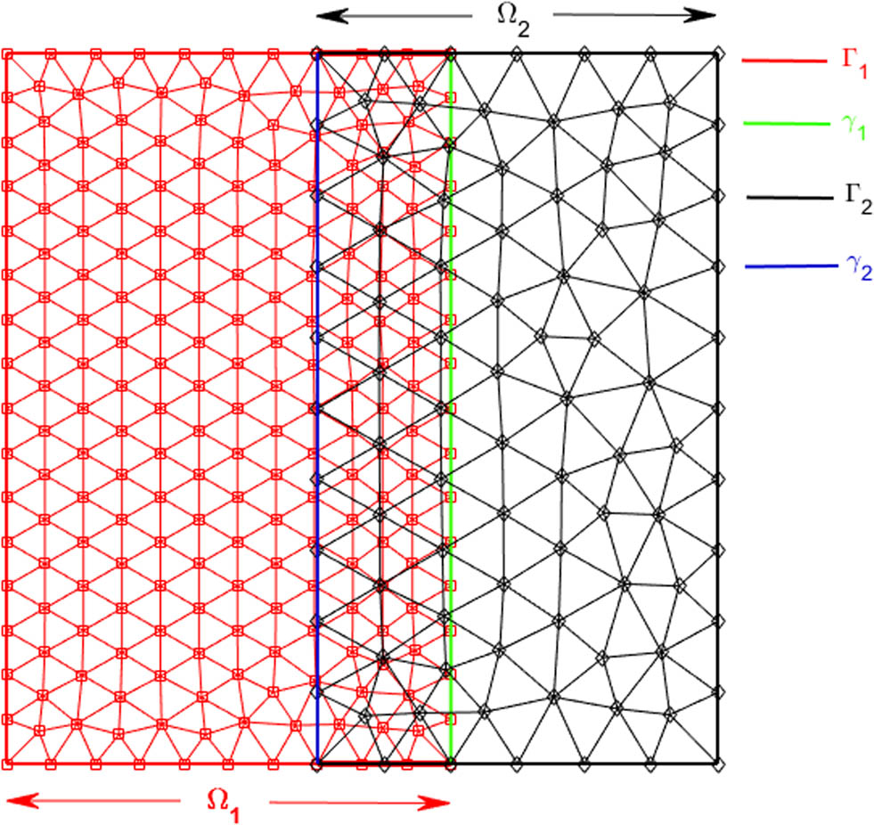
Example of quasi-uniform triangular non-matching meshes on two overlapping subdomains.

4 L ∞ -convergence analysis

This section is devoted to proving the main result of this article. For that, we first introduce the finite element counterparts of subproblems (3.1) and prove a key lemma.

4.1 Finite elements counterparts of subproblems (3.1)

For u ˜ i h i 0 = u i h i 0 ; i = 1 , 2 , we define the discrete sequences ( u ˜ i h i n ) such that u ˜ i h i n ∈ V h i solves

(4.1) a i ( u ˜ i h i n , v ) = ( F ( u i n − 1 ) , v ) ∀ v ∈ V ˚ h i u ˜ i h i n = π h i ( u n − 1 ) on γ i u ˜ i h i n = κ h i g on Γ i ,

where

u n ( x ) = max 1 ≤ i ≤ 2 u i n ( x ) , x ∈ Ω ¯ ,

and ( u i n ) is the Schwarz sequence defined in (3.1). Since u ˜ i h i n is the finite element approximation of u i n ; i = 1 , 2 , then we have the following lemma:

Lemma 2

[20] Assume that

∥ u i n + 1 ∥ W 2 , p ( Ω i ) ≤ C ; i = 1 , 2 .

Then we have

∥ u i n − u ˜ i h i n ∥ L ∞ ( Ω i ) ≤ C h 2 ∣ ln h ∣ .

Notation 2

For the sake of simplicity, we shall adopt the following notations in the proof of lemma 3:

∥ ⋅ ∥ 1 = ∥ ⋅ ∥ L ∞ ( Ω 1 ) ; ∣ ⋅ ∣ 1 = ∥ ⋅ ∥ L ∞ ( γ 1 ) , ∥ ⋅ ∥ 2 = ∥ ⋅ ∥ L ∞ ( Ω 2 ) ; ∣ ⋅ ∣ 2 = ∥ ⋅ ∥ L ∞ ( γ 2 ) , π h 1 = π h 2 = π h ,

and

h = max ( h 1 , h 2 ) .

4.2 The main result

The proof of the main result stands on the following crucial lemma whose proof can be found in Appendix A.

Lemma 3

Assume that f ( ⋅ ) is a Lipschitz continuous function, i.e., there is a constant k > 0 such that

(4.2) ∣ f ( x ) − f ( y ) ∣ ≤ k ∣ x − y ∣ ∀ x , y ∈ R .

Then, we have

(4.3) ∥ u 1 n − u 1 h n ∥ 1 ≤ 1 − ρ n + 1 1 − ρ ∑ i = 0 n ∥ u 1 i − u ˜ 1 h i ∥ 1 + 1 − ρ n 1 − ρ ∑ i = 0 n − 1 ∥ u 2 i − u ˜ 2 h i ∥ 2 ,

and

(4.4) ∥ u 2 n − u 2 h n ∥ 2 ≤ 1 − ρ n 1 − ρ ∑ i = 0 n − 1 ∥ u 1 i − u ˜ 1 h i ∥ 1 + 1 − ρ n + 1 1 − ρ ∑ i = 0 n ∥ u 2 i − u ˜ 2 h i ∥ 2 ,

where

ρ = k + c o β .

We are now in a position to prove the main result of this article.

Theorem 2

There exists h i , n > 0 with h i , n → 0 as n → ∞ , such that

(4.5) lim n → ∞ ∥ u i − u i h i , n n ∥ i = 0 ; i = 1 , 2 .

Proof

Let us give the proof for subdomain Ω 1 . The case of subdomain Ω 2 is similar. Indeed, we know that

∥ u 1 − u 1 h 1 , n n ∥ 1 ≤ ∥ u 1 − u 1 n ∥ 1 + ∥ u 1 n − u 1 h 1 , n n ∥ 1 .

Letting ε > 0 , Theorem 1 implies that there exists N ∈ N such that

∥ u 1 − u 1 n ∥ 1 ≤ ε 2 ∀ n > N .

On the other hand, since

∥ u 1 n − u 1 h 1 , n n ∥ 1 ≤ 1 − ρ n + 1 1 − ρ ∑ i = 0 n ∥ u 1 i − u ˜ 1 h 1 , n i ∥ 1 + 1 − ρ n 1 − ρ ∑ i = 0 n − 1 ∥ u 2 i − u ˜ 2 h 2 , n i ∥ 2 ≤ 1 − ρ n + 1 1 − ρ ∑ i = 0 n ∥ u 1 i − u ˜ 1 h n i ∥ 1 + 1 − ρ n 1 − ρ ∑ i = 0 n − 1 ∥ u 2 i − u ˜ 2 h n i ∥ 2 ,

and

∥ u i n − u ˜ i h n n ∥ i ≤ C h n 2 ∣ ln h n ∣ ; i = 1 , 2 ,

where h n = max { h 1 , n , h 2 , n } . Then,

∥ u 1 n − u 1 h 1 , n n ∥ 1 ≤ 1 − ρ n + 1 1 − ρ ( n + 1 ) C h n 2 ∣ ln h n ∣ + 1 − ρ n 1 − ρ n C h n 2 ∣ ln h n ∣ ≤ C I n h n 2 ∣ ln h n ∣ ,

where

I n = 1 − ρ n + 1 1 − ρ ( n + 1 ) + 1 − ρ n 1 − ρ n .

Thus, (4.5) follows by choosing h n > 0 such that

□ h n 2 ∣ ln h n ∣ ≤ ε 2 I n C ∀ n > N .

5 Numerical experiments

In this section, we perform a series of numerical experiments to support the theoretical results. To solve the semi linear problem, we use the linear additive Schwarz algorithm. For this purpose, we adapt a finite element code using the software “FreeFEM++” [22].

We consider the problem: find u such that

(5.1) − Δ u = − u 2 in Ω u = 12 ( x + y + 1 ) 2 on ∂ Ω ,

where Ω = [ 0 , 1 ] × [ 0 , 1 ] for all experiments. The exact solution (5.1) is shown in Figure 2(a), and it reads

u = 12 ( x + y + 1 ) 2 .

Figure 2

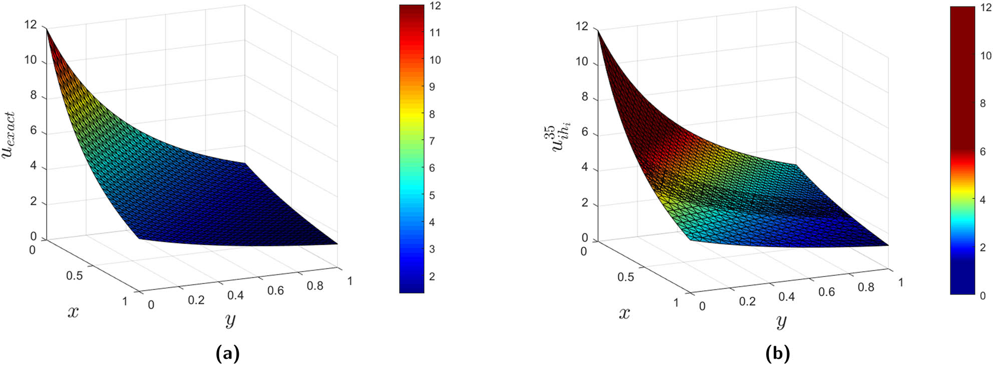
(a) The exact solution and (b) the numerical solution for n = 35 .

The coefficient c appearing in the discrete subproblem (3.4) is chosen such that the one-sided Lipschitz condition (2.13) is satisfied. Once determining suitable sector of lower and upper solutions to the problem, here ⟨ u ˇ , u ˆ ⟩ = ⟨ 0 , 12 ⟩ [21], the value of c is then determined by

(5.2) c ≡ sup { − f u ( x , u ) ; x ∈ Ω ¯ , u ˇ ≤ u ≤ u ˆ on Ω ¯ } = 24 .

Each subdomain is independently discretized with a linear quasi-uniform mesh triangular elements and different mesh size. As a consequence, the resulting grid in the intersection region between the two subdomains is non-matching. To satisfy the DMP, FreeFEM++ uses a variable metric/Delaunay automatic meshing algorithm accounting for the maximum edge length for every element K ∈ T h i ; i = 1 , 2 .

Initial results show the overall behavior of the proposed Schwarz algorithm. The first experiment is done by splitting the domain Ω into the two overlapping subdomains Ω 1 = 0 , 3 5 × [ 0 , 1 ] and Ω 2 = 2 5 , 1 × [ 0 , 1 ] with an overlap size δ = 1 5 . The mesh sizes used are h 1 = 1 30 and h 2 = 1 20 . As initial guess for the iterative process, we set u 1 h 0 and u 2 h 0 to be the subsolution u ˇ = 0 . Figure 2(b) represents the numerical solution in the 35th iteration. It is shown that the algorithm is able to deliver a quite good numerical approximation of the exact solution even though the initial guess is a bit farfetched.

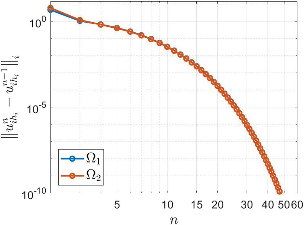
Furthermore, the monotone convergence of the discrete Schwarz sequences u i h i n is examined by evaluating the extrema of difference between two consecutive approximate solutions. If the extrema values are positive decreasing in n , a monotone convergence is numerically evident. Figure 3 represents the maximum values of the difference on both subdomains where a monotone convergence is observed.

Figure 3

Monotone convergence.

In the following numerical experiments, we investigate the effect of different parameters on the convergence of the discrete Schwarz sequences.

5.1 The effect of changing mesh size h i as n increases

This experiment is devoted for numerically proving Theorem 2. As it states, the mesh size h i , n is a nonincreasing function in n (i.e., h i , n → 0 as n → ∞ ). The main idea of the algorithm verifying the theory is that at the beginning of each iteration n , both subdomains are re-meshed with a finer mesh of size h i , n . The discrete sequences from the previous iteration (i.e., u i , h i , ( n − 1 ) ( n − 1 ) ) are linearly interpolated from the coarse mesh (i.e., h i , ( n − 1 ) ) to the current refined mesh (i.e., h i , n ) to obtain u i , h i , n ( n − 1 ) . The remaining additive Schwarz algorithm steps remain unchanged. Algorithm 1 describes the steps performed within each iteration.

Algorithm 1: Effect of simultaneously changing h i as n increases
n ← 1 , u 1 h 1 , 1 0 ← 0 , u 2 h 2 , 1 0 ← 0
while n < n max do
h 1 , n = 1 2 n + 1 , h 2 , n = 1 4 n + 1
Re-mesh subdomains:
Mesh Ω i with quasi-uniform triangular finite elements of size h i , n .
Define boundary conditions (BCs):
Impose the BC function g on Γ i .
Interpolate discrete sequences:
Interpolate the discrete sequence u 1 , h 1 , ( n − 1 ) ( n − 1 ) to get u 1 , h 1 , n ( n − 1 ) .
Interpolate the discrete sequence u 2 , h 2 , ( n − 1 ) ( n − 1 ) to get u 2 , h 2 , n ( n − 1 ) .
Solve subproblems:
Apply prolongation operators on the solutions ( u 1 h 1 , n n − 1 ) and ( u 2 h 2 , n n − 1 ) to obtain the BC on γ 1 and γ 2
Solve in parallel the linear systems corresponding to both subproblems to obtain u 1 h 1 , n n and u 2 h 2 , n n
n ← n + 1

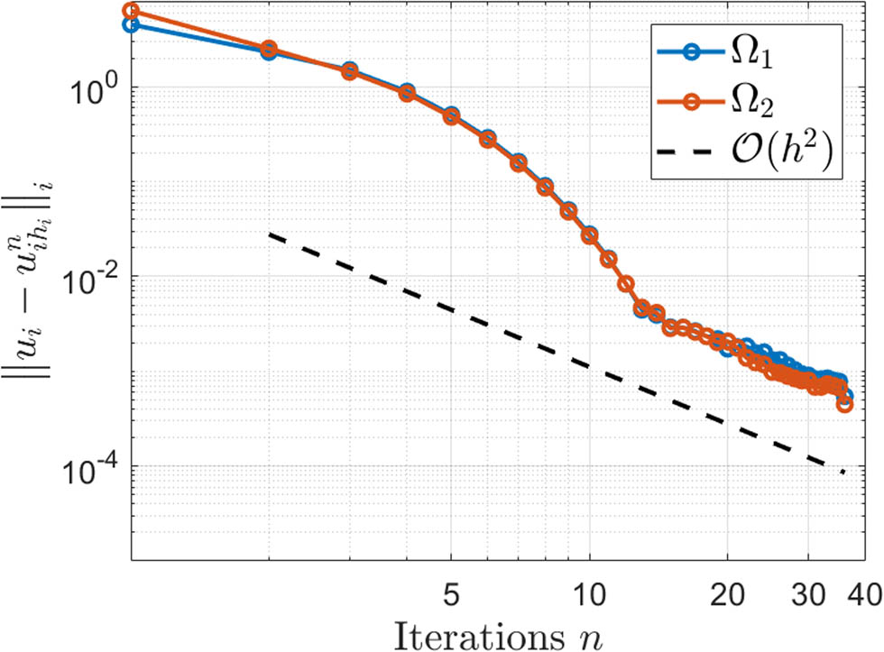
Here, we consider the domain Ω such that the overlapping subdomains are decomposed into Ω 1 = 0 , 5 8 × [ 0 , 1 ] and Ω 2 = 3 8 , 1 × [ 0 , 1 ] , leading to a fixed overlap size of δ = 1 4 . The mesh sizes employed in each subdomain are defined by h 1 , n = 1 2 n + 1 , and h 2 , n = 1 4 n + 1 , respectively. At the end of each iteration, the maximum norm error defined as ∥ u i − u i h i , n n ∥ i ; i = 1 , 2 , is evaluated and represented in Figure 4 for n = 1 , … , 36 . A continuous increase in the rate of convergence is initially observed. Once a certain iteration is reached (here, n = 13 ), the error tends to converge at a second-order rate of convergence.

Figure 4

Numerical validation of Theorem 2.

5.2 The effect of mesh size h i

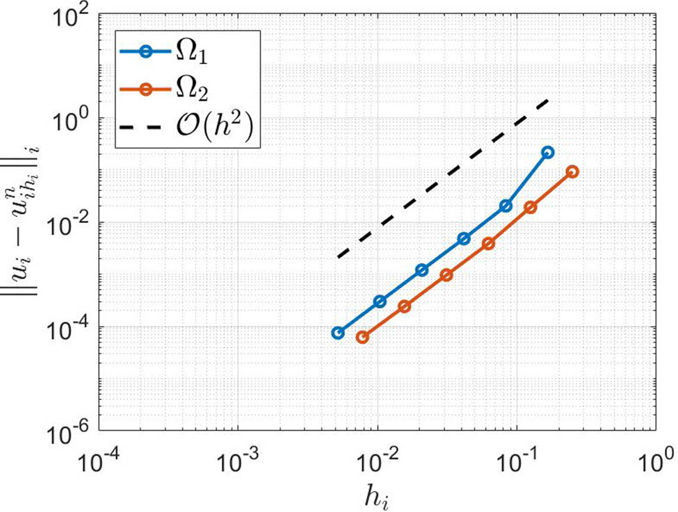
In this experiment, the overlapping subdomains setup here is similar to that employed in the previous subsection except the mesh sizes are chosen to be h 1 = 1 6 × 2 − l in Ω 1 , and h 2 = 1 4 × 2 − l in Ω 2 , where l = 0 , … , 5 is the level of refinement. Here, the number of Schwarz iterations performed for each mesh size h i on both subdomains should not be exceeded by the stopping criterion ε stop = 1 × 1 0 − 6 . Once ε stop is tolerated, the maximum norm error defined as ∥ u i − u i h i n ∥ i ; i = 1 , 2 , is evaluated. According to the obtained errors on both subdomains, Figure 5 depicts that a second-order rate of convergence is ensured.

Figure 5

Meshsizes versus maximum errors.

5.3 The effect of the overlap size δ

The effect of the overlap size δ on the additive Schwarz algorithm is examined by varying its value as δ i = 0.05 × i for i = 1 , … , 10 . However, mesh sizes in both subdomains are kept fixed to h 1 = 1 64 and h 2 = 1 48 . The convergence criteria of the Schwarz algorithm is set to ε stop = 1 × 1 0 − 6 . Once the Schwarz algorithm runs, δ is incremented in each step by 0.05 until a maximum value of 0.5 is reached. Therefore, the extended subdomains can be easily expressed as functions of δ i by Ω 1 , i = [ 0 , ( 0.5 + δ i ⁄ 2 ) ] × [ 0 , 1 ] and Ω 2 , i = [ ( 0.5 − δ i ⁄ 2 ) , 1 ] × [ 0 , 1 ] . Figure 6 represents the maximum number of iterations n required by the algorithm to reach convergence for each of the investigated overlap sizes δ i . It can be initially noticed a sharp decline in n as δ i increases followed by a steady decrease until almost no dependency is actually apparent.

Figure 6

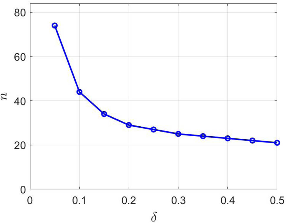
Effect of the overlap size.

6 Conclusion

We have shown mathematically and numerically the convergence of the standard finite element approximation of linear monotone additive Schwarz procedure for semilinear scalar elliptic PDEs, in the context of nonmatching grids. To prove the main result, we estimated, at each iteration, the error between the continuous and discrete Schwarz additive sequences. Moreover, we conducted several numerical experiments to validate our theoretical findings. The numerical results proved the monotone convergence of the discrete additive Schwarz sequences by monitoring the maximum values of the difference between consecutive discrete Schwarz iterations. Some numerical experiments were extended to investigate the effect of some parameters on the error defined as the maximum norm between the exact solution and the discrete Schwarz sequences. The numerical experiments have also provided a second-order convergence.

Acknowledgement

The authors extend their gratitude to Sultan Qaboos University for providing excellent research facilities and financial support for the publication fees.

Funding information: This work has not received any external funding.
Author contributions: All authors have accepted responsibility for the entire content of this manuscript and consented to its submission to the journal, reviewed all the results and approved the final version of the manuscript. Messaoud Boulbrachene handled the mathematical analysis part, while Qais Al Farei did the numerical analysis and numerical experimentation parts.
Conflict of interest: The authors declare that there is no conflict of interest.
Data availability statement: Data sharing is not applicable to this article as no datasets were generated or analysed during the current study.
Images: We confirm that all images contained in this manuscript are original.

Appendix A The proof of lemma 3

Proof

The proof will be carried out by induction. Also, we shall ignore the boundary condition on Γ i ; i = 1 , 2 as it does not affect our results.

Indeed, for [ n = 1 in Ω 1 ] , by making use of (2.8) and (4.2), we have

∥ u 1 1 − u 1 h 1 ∥ 1 ≤ ∥ u 1 1 − u ˜ 1 h 1 ∥ 1 + ∥ u ˜ 1 h 1 − u 1 h 1 ∥ 1 ≤ ∥ u 1 1 − u ˜ 1 h 1 ∥ 1 + max 1 β ∥ F ( u 1 0 ) − F ( u 1 h 0 ) ∥ 1 ; ∣ π h ( u 0 − u h 0 ) ∣ 1 ≤ ∥ u 1 1 − u ˜ 1 h 1 ∥ 1 + max { ρ ∥ u 1 0 − u 1 h 0 ∥ 1 ; ∣ u 0 − u h 0 ∣ 1 } .

Here, we need to consider the following two cases:

1 : max { ρ ∥ u 1 0 − u 1 h 0 ∥ 1 ; ∣ u 0 − u h 0 ∣ 1 } = ρ ∥ u 1 0 − u 1 h 0 ∥ 1 ,

2 : max { ρ ∥ u 1 0 − u 1 h 0 ∥ 1 ; ∣ u 0 − u h 0 ∣ 1 } = ∣ u 0 − u h 0 ∣ 1 .

Case 1 implies that

∥ u 1 1 − u 1 h 1 ∥ 1 ≤ ∥ u 1 1 − u ˜ 1 h 1 ∥ 1 + ρ ∥ u 1 0 − u 1 h 0 ∥ 1 ≤ ∥ u 1 1 − u ˜ 1 h 1 ∥ 1 + ρ ∥ u 1 0 − u ˜ 1 h 0 ∥ 1 ≤ ( 1 + ρ ) ∑ i = 0 1 ∥ u 1 i − u ˜ 1 h i ∥ 1 ,

while case 2 implies that

∥ u 1 1 − u 1 h 1 ∥ 1 ≤ ∥ u 1 1 − u ˜ 1 h 1 ∥ 1 + ∣ u 0 − u h 0 ∣ 1 ≤ ∥ u 1 1 − u ˜ 1 h 1 ∥ 1 + ∥ u 2 0 − u 2 h 0 ∥ 2 ≤ ∥ u 1 1 − u ˜ 1 h 1 ∥ 1 + ∥ u 2 0 − u ˜ 2 h 0 ∥ 2

because u 0 = u 2 0 , u h 0 = u 2 h 0 in Ω 2 .

Thus, both cases give

(A1) ∥ u 1 1 − u 1 h 1 ∥ 1 ≤ ( 1 + ρ ) ∑ i = 0 1 ∥ u 1 i − u ˜ 1 h i ∥ 1 + ∥ u 2 0 − u ˜ 2 h 0 ∥ 2 .

For [ n = 1 in Ω 2 ], by making use of (2.8) and (4.2) again, we have

∥ u 2 1 − u 2 h 1 ∥ 2 ≤ ∥ u 2 1 − u ˜ 2 h 1 ∥ 2 + ∥ u ˜ 2 h 1 − u 2 h 1 ∥ 2 ≤ ∥ u 2 1 − u ˜ 2 h 1 ∥ 2 + max 1 β ∥ F ( u 2 0 ) − F ( u 2 h 0 ) ∥ 2 ; ∣ π h ( u 0 − u h 0 ) ∣ 2 ≤ ∥ u 2 1 − u ˜ 2 h 1 ∥ 2 + max { ρ ∥ u 2 0 − u 2 h 0 ∥ 2 ; ∣ u 0 − u h 0 ∣ 2 } .

Again, we need to consider the following two cases:

1 : max { ρ ∥ u 2 0 − u 2 h 0 ∥ 2 ; ∣ u 0 − u h 0 ∣ 2 } = ρ ∥ u 2 0 − u 2 h 0 ∥ 2 ,

2 : max { ρ ∥ u 2 0 − u 2 h 0 ∥ 2 ; ∣ u 0 − u h 0 ∣ 2 } = ∣ u 0 − u h 0 ∣ 2 .

Case 1 implies that

∥ u 2 1 − u 2 h 1 ∥ 2 ≤ ∥ u 2 1 − u ˜ 2 h 1 ∥ 2 + ρ ∥ u 2 0 − u 2 h 0 ∥ 2 ≤ ∥ u 2 1 − u ˜ 2 h 1 ∥ 2 + ρ ∥ u 2 0 − u ˜ 2 h 0 ∥ 2 ≤ ( 1 + ρ ) ∑ i = 0 1 ∥ u 2 i − u ˜ 2 h i ∥ 2 ,

while case 2 implies that

∥ u 2 1 − u 2 h 1 ∥ 2 ≤ ∥ u 2 1 − u ˜ 2 h 1 ∥ 2 + ∣ u 0 − u h 0 ∣ 2 ≤ ∥ u 2 1 − u ˜ 2 h 1 ∥ 2 + ∥ u 1 0 − u 1 h 0 ∥ 1 ≤ ∥ u 2 1 − u ˜ 2 h 1 ∥ 2 + ∥ u 1 0 − u ˜ 1 h 0 ∥ 1

because u 0 = u 1 0 , u h 0 = u 1 h 0 in Ω 1 .

Thus, both cases give

(A2) ∥ u 2 1 − u 2 h 1 ∥ 2 ≤ ∥ u 1 0 − u ˜ 1 h 0 ∥ 1 + ( 1 + ρ ) ∑ i = 0 1 ∥ u 2 i − u ˜ 2 h i ∥ 2 .

For [ n = 2 in Ω 1 ], we obtain

∥ u 1 2 − u 1 h 2 ∥ 1 ≤ ∥ u 1 2 − u ˜ 1 h 2 ∥ 1 + ∥ u ˜ 1 h 2 − u 1 h 2 ∥ 1 ≤ ∥ u 1 2 − u ˜ 1 h 2 ∥ 1 + max 1 β ∥ F ( u 1 1 ) − F ( u 1 h 1 ) ∥ 1 ; ∣ π h ( u 1 − u h 1 ) ∣ 1 ≤ ∥ u 1 2 − u ˜ 1 h 2 ∥ 1 + max { ρ ∥ u 1 1 − u 1 h 1 ∥ 1 ; ∣ u 1 − u h 1 ∣ 1 } .

We then have to distinguish between two cases

1 : max { ρ ∥ u 1 1 − u 1 h 1 ∥ 1 ; ∣ u 1 − u h 1 ∣ 1 } = ρ ∥ u 1 1 − u 1 h 1 ∥ 1 ,

2 : max { ρ ∥ u 1 1 − u 1 h 1 ∥ 1 ; ∣ u 1 − u h 1 ∣ 1 } = ∣ u 1 − u h 1 ∣ 1 .

Using (A1), case 1 implies that

∥ u 1 2 − u 1 h 2 ∥ 1 ≤ ∥ u 1 2 − u ˜ 1 h 2 ∥ 1 + ρ ∥ u 1 1 − u 1 h 1 ∥ 1 ≤ ∥ u 1 2 − u ˜ 1 h 2 ∥ 1 + ρ ( 1 + ρ ) ∑ i = 0 1 ∥ u 1 i − u ˜ 1 h i ∥ 1 + ∥ u 2 0 − u ˜ 2 h 0 ∥ 2 ≤ ∥ u 1 2 − u ˜ 1 h 2 ∥ 1 + ( ρ + ρ 2 ) ∑ i = 0 1 ∥ u 1 i − u ˜ 1 h i ∥ 1 + ρ ∥ u 2 0 − u ˜ 2 h 0 ∥ 2 ≤ ( 1 + ρ + ρ 2 ) ∑ i = 0 2 ∥ u 1 i − u ˜ 1 h i ∥ 1 + ρ ∥ u 2 0 − u ˜ 2 h 0 ∥ 2 ,

while case 2 implies that

∥ u 1 2 − u 1 h 2 ∥ 1 ≤ ∥ u 1 2 − u ˜ 1 h 2 ∥ 1 + ∣ u 1 − u h 1 ∣ 1 .

But ∣ u 1 − u h 1 ∣ 1 has 4 possible subcases.

(a)

u 1 ( x ) = u 1 1 ( x ) and u h 1 ( x ) = u 1 h 1 ( x ) for x ∈ γ 1 , yield

∣ u 1 ( x ) − u h 1 ( x ) ∣ 1 = ∣ u 1 1 ( x ) − u 1 h 1 ( x ) ∣ 1 = ∣ u 0 ( x ) − u h 0 ( x ) ∣ 1 ≤ ∥ u 2 0 − u 2 h 0 ∥ 2 ,

(b)

u 1 ( x ) = u 1 1 ( x ) and u h 1 ( x ) = u 2 h 1 ( x ) for x ∈ γ 1 , yield

∣ u 1 ( x ) − u h 1 ( x ) ∣ 1 = ∣ u 1 1 ( x ) − u 2 h 1 ( x ) ∣ 1 ≤ ∣ u 1 1 ( x ) − u 1 h 1 ( x ) ∣ 1 ≤ ∥ u 2 0 − u 2 h 0 ∥ 2

because 0 ≤ u 1 h 1 ( x ) ≤ u 2 h 1 ( x ) .

(c)

u 1 ( x ) = u 2 1 ( x ) and u h 1 ( x ) = u 1 h 1 ( x ) for x ∈ γ 1 , yield

∣ u 1 ( x ) − u h 1 ( x ) ∣ 1 = ∣ u 2 1 ( x ) − u 1 h 1 ( x ) ∣ 1 ≤ ∣ u 2 1 ( x ) − u 2 h 1 ( x ) ∣ 1 ≤ ∥ u 2 1 − u 2 h 1 ∥ 2

because 0 ≤ u 2 h 1 ( x ) ≤ u 1 h 1 ( x ) .

(d)

u 1 ( x ) = u 2 1 ( x ) and u h 1 ( x ) = u 2 h 1 ( x ) for x ∈ γ 1 , yield

∣ u 1 ( x ) − u h 1 ( x ) ∣ 1 = ∣ u 2 1 ( x ) − u 2 h 1 ( x ) ∣ 1 ≤ ∥ u 2 1 − u 2 h 1 ∥ 2 .

From all the previous subcases, we can say that

∣ u 1 − u h 1 ∣ 1 = max ∣ u 1 ( x ) − u h 1 ( x ) ∣ 1 ∀ x ∈ γ 1 ≤ max { ∥ u 2 0 − u 2 h 0 ∥ 2 ; ∥ u 2 1 − u 2 h 1 ∥ 2 } .

So, by using (A2), we obtain

∥ u 1 2 − u 1 h 2 ∥ 1 ≤ ∥ u 1 2 − u ˜ 1 h 2 ∥ 1 + ∥ u 1 0 − u ˜ 1 h 0 ∥ 1 + ( 1 + ρ ) ∑ i = 0 1 ∥ u 2 i − u ˜ 2 h i ∥ 2 .

Thus, both cases yield

(A3) ∥ u 1 2 − u 1 h 2 ∥ 1 ≤ ( 1 + ρ + ρ 2 ) ∑ i = 0 2 ∥ u 1 i − u ˜ 1 h i ∥ 1 + ( 1 + ρ ) ∑ i = 0 1 ∥ u 2 i − u ˜ 2 h i ∥ 2 ≤ 1 − ρ 3 1 − ρ ∑ i = 0 2 ∥ u 1 i − u ˜ 1 h i ∥ 1 + 1 − ρ 2 1 − ρ ∑ i = 0 1 ∥ u 2 i − u ˜ 2 h i ∥ 2 .

For [ n = 2 in Ω 2 ] , we similarly have

∥ u 2 2 − u 2 h 2 ∥ 2 ≤ ∥ u 2 2 − u ˜ 2 h 2 ∥ 2 + ∥ u ˜ 2 h 2 − u 2 h 2 ∥ 2 ≤ ∥ u 2 2 − u ˜ 2 h 2 ∥ 2 + max 1 β ∥ F ( u 2 1 ) − F ( u 2 h 1 ) ∥ 2 ; ∣ π h ( u 1 − u h 1 ) ∣ 2 ≤ ∥ u 2 2 − u ˜ 2 h 2 ∥ 2 + max { ρ ∥ u 2 1 − u 2 h 1 ∥ 2 ; ∣ u 1 − u h 1 ∣ 2 } .

As mentioned earlier, we have two possible cases

1 : max { ρ ∥ u 2 1 − u 2 h 1 ∥ 2 ; ∣ u 1 − u h 1 ∣ 2 } = ρ ∥ u 2 1 − u 2 h 1 ∥ 2 ,

2 : max { ρ ∥ u 2 1 − u 2 h 1 ∥ 2 ; ∣ u 1 − u h 1 ∣ 2 } = ∣ u 1 − u h 1 ∣ 2 .

From (A2), case 1 implies that

∥ u 2 2 − u 2 h 2 ∥ 2 ≤ ∥ u 2 2 − u ˜ 2 h 2 ∥ 2 + ρ ∥ u 2 1 − u 2 h 1 ∥ 2 ≤ ∥ u 2 2 − u ˜ 2 h 2 ∥ 2 + ρ ∥ u 1 0 − u ˜ 1 h 0 ∥ 1 + ( 1 + ρ ) ∑ i = 0 1 ∥ u 2 i − u ˜ 2 h i ∥ 2 ≤ ∥ u 2 2 − u ˜ 2 h 2 ∥ 2 + ρ ∥ u 1 0 − u ˜ 1 h 0 ∥ 1 + ( ρ + ρ 2 ) ∑ i = 0 1 ∥ u 2 i − u ˜ 2 h i ∥ 2 ≤ ρ ∥ u 1 0 − u ˜ 1 h 0 ∥ 1 + ( 1 + ρ + ρ 2 ) ∑ i = 0 2 ∥ u 2 i − u ˜ 2 h i ∥ 2 ,

whereas case 2 gives

∥ u 2 2 − u 2 h 2 ∥ 2 ≤ ∥ u 2 2 − u ˜ 2 h 2 ∥ 2 + ∣ u 1 − u h 1 ∣ 2 .

But ∣ u 1 − u h 1 ∣ 2 also has 4 possible subcases.

(a)

u 1 ( x ) = u 1 1 ( x ) and u h 1 ( x ) = u 1 h 1 ( x ) for x ∈ γ 2 , yield

∣ u 1 ( x ) − u h 1 ( x ) ∣ 2 = ∣ u 1 1 ( x ) − u 1 h 1 ( x ) ∣ 2 ≤ ∥ u 1 1 − u 1 h 1 ∥ 1 .

(b)

u 1 ( x ) = u 1 1 ( x ) and u h 1 ( x ) = u 2 h 1 ( x ) for x ∈ γ 2 , yield

∣ u 1 ( x ) − u h 1 ( x ) ∣ 2 = ∣ u 1 1 ( x ) − u 2 h 1 ( x ) ∣ 2 ≤ ∣ u 1 1 ( x ) − u 1 h 1 ( x ) ∣ 2 ≤ ∥ u 1 1 − u 1 h 1 ∥ 1

because 0 ≤ u 1 h 1 ( x ) ≤ u 2 h 1 ( x ) .

(c)

u 1 ( x ) = u 2 1 ( x ) and u h 1 ( x ) = u 1 h 1 ( x ) for x ∈ γ 2 , yield

∣ u 1 ( x ) − u h 1 ( x ) ∣ 2 = ∣ u 2 1 ( x ) − u 1 h 1 ( x ) ∣ 2 ≤ ∣ u 2 1 ( x ) − u 2 h 1 ( x ) ∣ 2 = ∣ u 0 ( x ) − u h 0 ( x ) ∣ 2 ≤ ∥ u 1 0 − u 1 h 0 ∥ 1

because 0 ≤ u 2 h 1 ( x ) ≤ u 1 h 1 ( x ) .

(d)

u 1 ( x ) = u 2 1 ( x ) and u h 1 ( x ) = u 2 h 1 ( x ) for x ∈ γ 2 , yield

∣ u 1 ( x ) − u h 1 ( x ) ∣ 2 = ∣ u 2 1 ( x ) − u 2 h 1 ( x ) ∣ 2 ≤ ∥ u 1 0 − u 1 h 0 ∥ 1 .

From all the previous subcases, we have

∣ u 1 − u h 1 ∣ 2 = max ∣ u 1 ( x ) − u h 1 ( x ) ∣ 2 ∀ x ∈ γ 2 ≤ max { ∥ u 1 1 − u 1 h 1 ∥ 1 ; ∥ u 1 0 − u 1 h 0 ∥ 1 } .

So, by using (A1), we obtain

∥ u 2 2 − u 2 h 2 ∥ 2 ≤ ( 1 + ρ ) ∑ i = 0 1 ∥ u 1 i − u ˜ 1 h i ∥ 1 + ∥ u 2 2 − u ˜ 2 h 2 ∥ 2 + ∥ u 2 0 − u ˜ 2 h 0 ∥ 2 .

Thus, in both cases, we obtain

(A4) ∥ u 2 2 − u 2 h 2 ∥ 2 ≤ ( 1 + ρ ) ∑ i = 0 1 ∥ u 1 i − u ˜ 1 h i ∥ 1 + ( 1 + ρ + ρ 2 ) ∑ i = 0 2 ∥ u 2 i − u ˜ 2 h i ∥ 2 ≤ 1 − ρ 2 1 − ρ ∑ i = 0 1 ∥ u 1 i − u ˜ 1 h i ∥ 1 + 1 − ρ 3 1 − ρ ∑ i = 0 2 ∥ u 2 i − u ˜ 2 h i ∥ 2 .

Now assume that both (4.3) and (4.4) hold. We need to prove the lemma for the ( n + 1 )th step in both subdomains. Indeed, on Ω 1 , using the same argument as above, we have

∥ u 1 n + 1 − u 1 h n + 1 ∥ 1 ≤ ∥ u 1 n + 1 − u ˜ 1 h n + 1 ∥ 1 + ∥ u ˜ 1 h n + 1 − u 1 h n + 1 ∥ 1 ≤ ∥ u 1 n + 1 − u ˜ 1 h n + 1 ∥ 1 + max { ρ ∥ u 1 n − u 1 h n ∥ 1 ; ∣ u n − u h n ∣ 1 } .

As above, we need to distinguish between two cases.

Case 1:

max { ρ ∥ u 1 n − u 1 h n ∥ 1 ; ∣ u n − u h n ∣ 1 } = ρ ∥ u 1 n − u 1 h n ∥ 1 .

By (4.3), this gives

∥ u 1 n + 1 − u 1 h n + 1 ∥ 1 ≤ ∥ u 1 n + 1 − u ˜ 1 h n + 1 ∥ 1 + ρ ∥ u 1 n − u 1 h n ∥ 1 ≤ ∥ u 1 n + 1 − u ˜ 1 h n + 1 ∥ 1 + ρ 1 − ρ n + 1 1 − ρ ∑ i = 0 n ∥ u 1 i − u ˜ 1 h i ∥ 1 + 1 − ρ n 1 − ρ ∑ i = 0 n − 1 ∥ u 2 i − u ˜ 2 h i ∥ 2 ≤ ∥ u 1 n + 1 − u ˜ 1 h n + 1 ∥ 1 + ρ ( 1 + … + ρ n ) ∑ i = 0 n ∥ u 1 i − u ˜ 1 h i ∥ 1 + ( 1 + … + ρ n − 1 ) ∑ i = 0 n − 1 ∥ u 2 i − u ˜ 2 h i ∥ 2 ≤ ∥ u 1 n + 1 − u ˜ 1 h n + 1 ∥ 1 + ( ρ + … + ρ n + 1 ) ∑ i = 0 n ∥ u 1 i − u ˜ 1 h i ∥ 1 + ρ ( 1 + … + ρ n − 1 ) ∑ i = 0 n − 1 ∥ u 2 i − u ˜ 2 h i ∥ 2 ≤ ( 1 + ρ + … + ρ n + 1 ) ∑ i = 0 n + 1 ∥ u 1 i − u ˜ 1 h i ∥ 1 + ρ ( 1 + … + ρ n − 1 ) ∑ i = 0 n − 1 ∥ u 2 i − u ˜ 2 h i ∥ 2 ≤ 1 − ρ n + 2 1 − ρ ∑ i = 0 n + 1 ∥ u 1 i − u ˜ 1 h i ∥ 1 + ρ ( 1 − ρ n 1 − ρ ) ∑ i = 0 n − 1 ∥ u 2 i − u ˜ 2 h i ∥ 2 .

Case 2:

max { ρ ∥ u 1 n − u 1 h n ∥ 1 ; ∣ u n − u h n ∣ 1 } = ∣ u n − u h n ∣ 1 ,

which gives

∥ u 1 n + 1 − u 1 h n + 1 ∥ 1 ≤ ∥ u 1 n + 1 − w 1 h n + 1 ∥ 1 + ∣ u n − u h n ∣ 1 .

But ∣ u n − u h n ∣ 1 has 4 possible subcases.

(a)

u n ( x ) = u 1 n ( x ) and u h n ( x ) = u 1 h n ( x ) for x ∈ γ 1 , yield

∣ u n ( x ) − u h n ( x ) ∣ 1 = ∣ u 1 n ( x ) − u 1 h n ( x ) ∣ 1 = ∣ u n − 1 ( x ) − u h n − 1 ( x ) ∣ 1 ≤ ∥ u 2 n − 1 − u 2 h n − 1 ∥ 2 .

(b)

u n ( x ) = u 1 n ( x ) and u h n ( x ) = u 2 h n ( x ) for x ∈ γ 1 , yield

∣ u n ( x ) − u h n ( x ) ∣ 1 = ∣ u 1 n ( x ) − u 2 h n ( x ) ∣ 1 ≤ ∣ u 1 n ( x ) − u 1 h n ( x ) ∣ 1 ≤ ∥ u 2 n − 1 − u 2 h n − 1 ∥ 2

since 0 ≤ u 1 h n ( x ) ≤ u 2 h n ( x ) .

(c)

u n ( x ) = u 2 n ( x ) and u h n ( x ) = u 1 h n ( x ) for x ∈ γ 1 , yield

∣ u n ( x ) − u h n ( x ) ∣ 1 = ∣ u 2 n ( x ) − u 1 h n ( x ) ∣ 1 ≤ ∣ u 2 n ( x ) − u 2 h n ( x ) ∣ 1 ≤ ∥ u 2 n − u 2 h n ∥ 2

since 0 ≤ u 2 h n ( x ) ≤ u 1 h n ( x ) .

(d)

u n ( x ) = u 2 n ( x ) and u h n ( x ) = u 2 h n ( x ) for x ∈ γ 1 , yield

∣ u n ( x ) − u h n ( x ) ∣ 1 = ∣ u 2 n ( x ) − u 2 h n ( x ) ∣ 1 ≤ ∥ u 2 n − u 2 h n ∥ 2 .

From all previous subcases of ∣ u n − u h n ∣ 1 , we obtain

∣ u n − u h n ∣ 1 = max ∣ u n ( x ) − u h n ( x ) ∣ 1 ∀ x ∈ γ 1 ≤ max { ∥ u 2 n − 1 − u 2 h n − 1 ∥ 2 ; ∥ u 2 n − u 2 h n ∥ 2 } .

As a consequence of (4.4), we have

∥ u 1 n + 1 − u 1 h n + 1 ∥ 1 ≤ ∥ u 1 n + 1 − u ˜ 1 h n + 1 ∥ 1 + ∥ u 2 n − u 2 h n ∥ 2 ≤ ∥ u 1 n + 1 − u ˜ 1 h n + 1 ∥ 1 + 1 − ρ n 1 − ρ ∑ i = 0 n − 1 ∥ u 1 i − u ˜ 1 h i ∥ 1 + 1 − ρ n + 1 1 − ρ ∑ i = 0 n ∥ u 2 i − u ˜ 2 h i ∥ 2 ≤ 1 − ρ n 1 − ρ ∑ i = 0 n + 1 ∥ u 1 i − u ˜ 1 h i ∥ 1 + 1 − ρ n + 1 1 − ρ ∑ i = 0 n ∥ u 2 i − u ˜ 2 h i ∥ 2 .

Hence, in both cases, we obtain

(A5) ∥ u 1 n + 1 − u 1 h n + 1 ∥ 1 ≤ 1 − ρ n + 2 1 − ρ ∑ i = 0 n + 1 ∥ u 1 i − u ˜ 1 h i ∥ 1 + 1 − ρ n + 1 1 − ρ ∑ i = 0 n ∥ u 2 i − u ˜ 2 h i ∥ 2 .

Likewise, we have in Ω 2

∥ u 2 n + 1 − u 2 h n + 1 ∥ 2 ≤ ∥ u 2 n + 1 − u ˜ 2 h n + 1 ∥ 2 + ∥ u ˜ 2 h n + 1 − u 2 h n + 1 ∥ 2 ≤ ∥ u 2 n + 1 − u ˜ 2 h n + 1 ∥ 2 + max { ρ ∥ u 2 n − u 2 h n ∥ 2 ; ∣ u n − u h n ∣ 2 } .

Again here, we need to discuss two cases.

Case 1:

max { ρ ∥ u 2 n − u 2 h n ∥ 1 ; ∣ u n − u h n ∣ 2 } = ρ ∥ u 2 n − u 2 h n ∥ 2

By (4.4), this gives

∥ u 2 n + 1 − u 2 h n + 1 ∥ 2 ≤ ∥ u 2 n + 1 − u ˜ 2 h n + 1 ∥ 2 + ρ ∥ u 2 n − u 2 h n ∥ 2 ≤ ∥ u 2 n + 1 − u ˜ 2 h n + 1 ∥ 2 + ρ 1 − ρ n 1 − ρ ∑ i = 0 n − 1 ∥ u 1 i − u ˜ 1 h i ∥ 1 + 1 − ρ n + 1 1 − ρ ∑ i = 0 n ∥ u 2 i − u ˜ 2 h i ∥ 2 ≤ ∥ u 2 n + 1 − u ˜ 2 h n + 1 ∥ 2 + ρ ( 1 + … + ρ n − 1 ) ∑ i = 0 n − 1 ∥ u 1 i − u ˜ 1 h i ∥ 1 + ( 1 + … + ρ n ) ∑ i = 0 n ∥ u 2 i − u ˜ 2 h i ∥ 2 ≤ ∥ u 2 n + 1 − u ˜ 2 h n + 1 ∥ 2 + ρ ( 1 + … + ρ n − 1 ) ∑ i = 0 n − 1 ∥ u 1 i − u ˜ 1 h i ∥ 1 + ( ρ + … + ρ n + 1 ) ∑ i = 0 n ∥ u 2 i − u ˜ 2 h i ∥ 2 ≤ ρ ( 1 + … + ρ n − 1 ) ∑ i = 0 n − 1 ∥ u 1 i − u ˜ 1 h i ∥ 1 + ( 1 + ρ + … + ρ n + 1 ) ∑ i = 0 n + 1 ∥ u 2 i − u ˜ 2 h i ∥ 2 ≤ ρ 1 − ρ n 1 − ρ ∑ i = 0 n − 1 ∥ u 1 i − u ˜ 1 h i ∥ 1 + 1 − ρ n + 2 1 − ρ ∑ i = 0 n + 1 ∥ u 2 i − u ˜ 2 h i ∥ 2

Case 2:

max { ρ ∥ u 2 n − u 2 h n ∥ 1 ; ∣ u n − u h n ∣ 2 } = ∣ u n − u h n ∣ 2

Similarly, after studying all subcases of ∣ u n − u h n ∣ 2 , we obtain

∣ u n − u h n ∣ 2 = max ∣ u n ( x ) − u h n ( x ) ∣ 2 ∀ x ∈ γ 2 ≤ max { ∥ u 1 n − u 1 h n ∥ 1 ; ∥ u 1 n − 1 − u 1 h n − 1 ∥ 1 } .

As a consequence of (4.3), this gives

∥ u 2 n + 1 − u 2 h n + 1 ∥ 2 ≤ ∥ u 2 n + 1 − u ˜ 2 h n + 1 ∥ 2 + ∥ u 1 n − u 1 h n ∥ 1 ≤ ∥ u 2 n + 1 − u ˜ 2 h n + 1 ∥ 2 + 1 − ρ n + 1 1 − ρ ∑ i = 0 n ∥ u 1 i − u ˜ 1 h i ∥ 1 + 1 − ρ n 1 − ρ ∑ i = 0 n − 1 ∥ u 2 i − u ˜ 2 h i ∥ 2 ≤ 1 − ρ n + 1 1 − ρ ∑ i = 0 n ∥ u 1 i − u ˜ 1 h i ∥ 1 + 1 − ρ n 1 − ρ ∑ i = 0 n + 1 ∥ u 2 i − u ˜ 2 h i ∥ 2 .

Hence, both cases yield

(A6) ∥ u 2 n + 1 − u 2 h n + 1 ∥ 2 ≤ 1 − ρ n + 1 1 − ρ ∑ i = 0 n ∥ u 1 i − u ˜ 1 h i ∥ 1 + 1 − ρ n + 2 1 − ρ ∑ i = 0 n + 1 ∥ u 2 i − u ˜ 2 h i ∥ 2 ,

which completes the proof.□

References

[1] Lions PL. On the Schwarz alternating method I. First international symposium on domain decomposition methods for partial differential equations. Philadelphia Pa, USA: SIAM; 1988. p. 1–40. Search in Google Scholar

[2] Lions PL. On the Schwarz alternating method II. Second international symposium on domain decomposition methods for partial differential equations. Philadelphia, Pa, USA: SIAM; 1989. p. 47–70. Search in Google Scholar

[3] Glowinski R, Golub GH, Meurant GA, Periaux J. Domain decomposition methods for partial differential equations. First international symposium on domain decomposition methods for partial differential equations. Philadelphia, PA, USA: SIAMl; 1988. Search in Google Scholar

[4] Dryja M, Widlund OB. An additive variant of the Schwarz alternating method for the case of many subregions. Technical report. Courant Institute technical report 339. 1987. Search in Google Scholar

[5] Lui SH. On Schwarz alternating methods for nonlinear elliptic PDEs. SISC. 1999;21(4):1506–23. 10.1137/S1064827597327553Search in Google Scholar

[6] Lui SH. On monotone and Schwarz alternating methods for nonlinear elliptic PDEs. ESAIM M2AN. 2001;35(1):1–15. 10.1051/m2an:2001104Search in Google Scholar

[7] Lui SH. On linear monotone iteration and Schwarz methods for nonlinear elliptic PDEs. Numer Math. 2002;93(1):109–29. 10.1007/BF02679439Search in Google Scholar

[8] Boulbrachene M, Cortey-Dumont Ph, Miellou JC. Mixing finite elements and finite differences in a subdomain method. First international symposium on domain decomposition methods for partial differential equations. Philadelphia, Pa, USA: SIAM; 1988. p. 198–216. Search in Google Scholar

[9] Boulbrachene M, Saadi S. Maximum norm analysis of an overlapping nonmatching grids method for the obstacle problem. Adv Differ Equations. 2006;2006:85807. 10.1155/ADE/2006/85807Search in Google Scholar

[10] Harbi A, Boulbrachene M. Maximum norm analysis of a non-matching grids method for nonlinear elliptic PDEs. J Appl Math. 2011;2011:605140.10.1155/2011/605140Search in Google Scholar

[11] Harbi A. Maximum norm analysis of an arbitrary number of non-matching grids method for nonlinear elliptic PDEs. J Appl Math. 2013;2013:893182.10.1155/2013/893182Search in Google Scholar

[12] Boulbrachene M, Al Farei Q. Maximum norm error analysis of a non-matching grids finite element method for linear PDEs. Appl Math Comput. 2014;238:21–9. 10.1016/j.amc.2014.03.146Search in Google Scholar

[13] Harbi A. Maximum norm analysis of a non-matching grids method for a class of variational inequalities with nonlinear source terms, J Inequal Appl. 2016;181:27. 10.1186/s13660-016-1110-4Search in Google Scholar

[14] Boulbrachene M. Finite element convergence analysis of Schwarz alternating method for nonlinear elliptic PDEs. SQUJS. 2019;24(2):109–21. 10.24200/squjs.vol24iss2pp109-121Search in Google Scholar

[15] Al Farei Q, Boulbrachene M. Mixing finite elements and finite differences in nonlinear Schwarz iterations for nonlinear elliptic PDEs. Comput Math Model. 2022;33(1):77–94. 10.1007/s10598-022-09558-xSearch in Google Scholar

[16] Al Farei Q, Boulbrachene M. L∞-Convergence analysis of a finite element linear Schwarz alternating method for a class of semi-linear elliptic PDEs. Int J Anal Appl. January 2023;21(71):1–28. 10.28924/2291-8639-21-2023-71Search in Google Scholar

[17] Ciarlet PG. Discrete maximum principle for finite-difference operators. Aequ Math. 1970;4(3):338–52. 10.1007/BF01844166Search in Google Scholar

[18] Ciarlet PG, Raviart PA. Maximum principle and uniform convergence for the finite element method. Comput Methods Appl Mech Eng. 1973;2(1):17–31. 10.1016/0045-7825(73)90019-4Search in Google Scholar

[19] Lu C, Huang W, Qiu J. Maximum principle in linear finite element approximations of anisotropic diffusion-convection-reaction problems. Numer Math. 2014;127:515–37. 10.1007/s00211-013-0595-8Search in Google Scholar

[20] Nitsche J. L∞-convergence of finite element approximations. In Proceedings of the symposium on mathematical aspects of finite element methods. Lectures notes in mathematics. Springer; Vol. 606; 1977. pp. 261–74. 10.1007/BFb0064468Search in Google Scholar

[21] Pao CV. Nonlinear parabolic and elliptic equations. New York: Plenum Press; 1992. 10.1007/978-1-4615-3034-3Search in Google Scholar

[22] Hecht F. New development in freefem++. J Numer Math. 2012;20(3–4):251–65. 10.1515/jnum-2012-0013Search in Google Scholar

Received: 2023-09-27

Revised: 2024-04-23

Accepted: 2024-05-21

Published Online: 2024-10-29

This work is licensed under the Creative Commons Attribution 4.0 International License.

Articles in the same Issue

https://doi.org/10.1515/nleng-2024-0016

Keywords for this article

semi-linear problem; additive Schwarz method; finite elements; nonmatching grids; uniform convergence

Creative Commons

BY 4.0