Determining the long-term impact area of coastal thermal discharge based on a harmonic model of sea surface temperature

Yin Yaqiu; Zhao Limin; Yang Hongyan; Yu Yang; Wang Jie; Yang Jinzhong

doi:10.1515/geo-2022-0471

Artikel Open Access

Determining the long-term impact area of coastal thermal discharge based on a harmonic model of sea surface temperature

Yin Yaqiu , Zhao Limin , Yang Hongyan , Yu Yang , Wang Jie und Yang Jinzhong

Veröffentlicht/Copyright: 6. April 2023

Veröffentlicht von

Veröffentlichen auch Sie bei De Gruyter Brill

Manuskript einreichen Informationen für Autor*innen

Aus der Zeitschrift Open Geosciences Band 15 Heft 1

Abstract

Coastal nuclear power plants discharge large amounts of warm cooling water, which may have environmental impacts. This study proposes a method for determining the long-term impact area based on the average distribution of sea surface temperate (SST) increases. Taking the Daya Bay Nuclear Power Plant as a case study, 101 TM/ETM+ images acquired from 2000 to 2013 were used to obtain SST products. Cross-validation with NR_2P products showed that the accuracy of the SST products, in terms of the systematic error, root-mean-square error, and mean absolute error of 1,000 randomly selected verification points, was all <0.3°C, while Willmott’s index of agreement values was all >0.7. An annual SST cycle harmonic model was established. The mean difference between the modeled and observed SSTs was −2.1 to 2.5°C with a standard deviation range of 0–1°C. The long-term impact area was extracted by the harmonic analysis method and multi-year average method for comparison. The following conclusions can be drawn: 1) with sufficient SST samples, the temperature distributions of the two methods are similar, with the multi-year average method giving less noise and clearer boundaries. 2) When SST data are lacking for some months, the mean and standard deviation of the percentage of pixels belonging to areas of different temperature rise were calculated. The standard deviations of the two methods were both <0.04 in the temperature-rise classes of 1–2, 2–3, 3–4, and 4–5°C, while in the 0–1°C class, the standard deviation of the multi-year average method was 0.461, which is much higher than that of the multi-year average method (0.098). Performing statistical analysis on all pixels of >0°C, the multi-year average method had a standard deviation of 0.506, while the harmonic analysis method had a value of 0.128. Overall, the harmonic analysis method makes it possible to obtain and evaluate the long-term stability impact area of the thermal discharge over a period of time comprehensively and quantitatively. Even though it introduces a small amount of noise, it has less dependence on the input SST products and could improve the stability and reliability of thermal discharge monitoring, providing technical support for precise pollution control.

Keywords: thermal infrared remote sensing; harmonic analysis method; the robust annual cycle parameters; thermal discharge long-term impact area; SST; Daya Bay Nuclear Power Station; TM/ETM+

1 Introduction

In recent years, nuclear power generation has become highly valued, as it is carbon emissions-free and could reduce the greenhouse effect significantly. At present, in China, the conversion efficiency of nuclear energy in nuclear power plants is only about 33%, and a large amount of excess heat must be discharged into natural coastal waters via circulating cooling water [1]. The temperature of discharged cooling water is usually 6–11°C above that of the ambient water; thus, its continuous discharge forms a kind of thermal pollution that may affect the quality of surrounding aquatic environments and the development and distribution of fish, plankton, and benthic organisms [2,3,4].

To manage the effects of thermal discharge on aquatic ecosystems, many countries believe that regions affected by thermal discharge should be predicted and observed to monitor and regulate thermal pollution. In the planning and design stages of nuclear power plants, physical and numerical simulations are often used to predict thermal discharge distributions under various conditions [5,6]. Large-area measurement and thermal infrared remote sensing are often used to observe and evaluate the impacts of thermal discharge during power plant operation. However, large-area measurement costs time and money and cannot objectively reflect the spatial distribution characteristics of thermal discharge [7,8]. In contrast, thermal infrared remote sensing has been widely used, as it can monitor sea surface temperatures (SSTs) at various spatial scales [9,10].

Thermal discharge from coastal nuclear power plants has particular characteristics as the outlet locations are fixed and the discharge of warm drainage accompanies the whole process of nuclear power production, so the environmental impacts accumulate over the long term. The distribution of thermal discharge changes over time. So, to comprehensively evaluate the scope and temperature distribution of thermal drainage within a period of time, the concept of long-term impact area should be introduced. In principle, the long-term impact area of thermal discharge is an average spatial distribution of the area of temperature rise caused by thermal discharge within a period of time, which is similar to the concept of the normal water level of the river [11]. However, most existing research on thermal infrared remote sensing is based on using singular or discrete data to determine the variations and characteristics of thermal discharge distributions. This fails to comprehensively determine the long-term impact area and distribution [12,13,14]. Recently, some scholars have extracted and analyzed thermal discharge impact areas from the perspective of long-time series data. For example, based on 70 views of HJ-1B and Landsat 7/8 satellites, Wang et al. proposed extracting the temperature rise envelope for a period of time to reflect the range of influence of cooling water by overlaying and combining the temperature isolines of several remote sensing images [15]. However, envelopes acquired by this method actually reflect the maximum range of temperature rise caused by thermal discharge within a period of time and cannot reflect long-term stable impact areas. The result has a degree of randomness and cannot meet the requirement of precise pollution control. Generally speaking, previous studies on the long-term impact area extraction by remote sensing method are limited by short-term and single time series data which cannot reflect the long-term influence on the one hand. And on the other hand, the extraction method is not scientific enough to extract the maximum probability of the influence range.

Nearshore SST is affected by solar radiation and shows an annual cycle, while thermal discharge disturbs this cycle. Through time-domain analysis of SST, the range and degree of such disturbance can be captured. Some scholars have used the frequency characteristics of remote sensing time series data to identify targets of periodic change [16,17,18]. Bechtel proposed robust annual cycle parameters (RACP) based on land surface temperature (LST) time series acquired by Landsat and proposed that characteristics like the LST mean, amplitude, and phase can quantify spatial heterogeneity in the urban heat island effect over a period of time [19]. Assuming repetitive temperature cycles, Fu and Weng optimized annual temperature cycle parameters using a sinusoidal function fitted to eight-day MODIS LST composite data to reveal differences in the annual temperature cycle (ATC) parameters of urban and rural areas and the impacts of surface urban heat islands on ATC ranges across the continental United States [20].

As there is a need for thermal discharge assessments for monitoring purposes, this study proposes a harmonic analysis method (HAM). It establishes an annual cycle harmonic model using SST time series to obtain RACPs and quantify areas of long-term thermal discharge impacts. The new method was compared with the multi-year average method (MAM) under different tidal conditions and SST datasets. The aim was to provide technical support for the monitoring and evaluation of thermal discharge effects around coastal nuclear power plants.

1.1 Study area and experimental data

This study examined the Daya Bay Nuclear Power Station (DNPS), which is located on the southeast side of Dapeng Peninsula, Dapeng New Area, Shenzhen City, Guangdong Province. It faces Dapengao Bay to the south, Daya Bay to the east, and mountains and hills to the north and west (Figure 1). Daya Bay is surrounded by numerous islands, which form natural barriers to make the bay stay calm all year round. Driven by these conditions, the annual variation in seawater is stable, which is beneficial for carrying out an SST phenological analysis.

Figure 1

Location of the Daya Bay Nuclear Power Station (DNPS).

The experimental data included 101 TM/ETM+ scenes (path/row: 121/44) with <20% cloud cover acquired in the study area from 2000 to 2013. The temporal distribution is shown in Figure 2. The SST inversion results were validated using 1,000 points from 13 scenes of the NR_2P products (2000–2012) of ATSR-2 (1995–2011) and ATSR (2002–2012) sensors on the ERS-2 and Envisat-1 satellites of the European Space Agency. Tidal data with 1-hour intervals were obtained from the Tidal Table published by the State Oceanic Administration.

Figure 2

Number of images acquired in each month.

The TM and ETM+ thematic mappers on the Landsat satellites have a thermal infrared band (band 6), the spatial resolutions of which are 120 and 60 m, respectively. The NR_2P products are secondary geographic products for ocean, land, and atmosphere data with a resolution of 1 km.

2 Model and methods

2.1 Research scheme

The technical route is shown in Figure 3. First, TM/ETM+ remote sensing images were used to obtain a long SST time series, and cross-validation was carried out based on the NR_2P products. Second, an annual cycle harmonic model was established to reconstruct the time series and obtain the RACPs, according to which the effects of cloud and tide were analyzed. Third, extraction of the long-term thermal discharge-affected area was carried out. The HAM and MAM were both used to extract the long-term affected area, with the results of different tidal conditions and SST distributions used for comparison and evaluation.

Figure 3

Technical route map.

2.2 Single-channel thermal infrared SST inversion and verification

Under cloud-free conditions, the atmosphere can be considered approximately horizontally homogeneous and isotropic, and the atmospheric boundary layer satisfies the local thermal equilibrium state. For the thermal infrared band, when the viewing angle of the sensor is <50°, the ocean surface can be approximately treated as a Lambert reflector, and the thermal infrared radiation received by the sensor includes information from the sun, underlying surface and atmosphere. According to the principle of radiative transfer, as shown in Formula (1) [21], the SST can be expressed as a function of the seawater emissivity ε _λ, the total radiation R of the thermal infrared channels received by the sensors, the upward radiation L ^↑ _λ and downward radiation L ^↓ _λ of the atmosphere, and the atmospheric transmittance t _λ. Because water can absorb the most radiation, the seawater emissivity is approximately 1, so SST can be acquired if the R, L ^↑ _λ, L ^↓ _λ, and t _λ of the study area are known.

(1) SST = f ( ε λ , R , L λ ↑ , L λ ↓ , t λ ) .

Radiometric calibration, ETM+ strip restoration, geometric correction, atmospheric correction, land masking, and other data processes were carried out on the 101 scenes of TM/ETM+ data. Parameter R of the thermal infrared channels was obtained through radiometric calibration, and the atmospheric correction of TM/ETM+ thermal infrared data was completed using an online atmospheric correction tool (atmcorr.gsfc.nasa.gov), based on the atmospheric profile of NCEP reanalyzed data, to acquire L ^↑ _λ, L ^↓ _λ, and t _λ. With the obtained parameters (as shown in Figure 4), and using the MODerate spectral resolution atmospheric TRANsmittance software and program IDL, SST products were obtained and uniformly sampled to a spatial resolution of 60 m. So the spatial resolutions of the subsequently extracted and analyzed results based on the SST products were also 60 m. The sampling strategy proposed by Feng et al. was adopted to reduce the influence of spatial resolution differences during verification, and the threshold value of the variance was set as 0.3k [22].

Figure 4

Temporal distribution of atmospheric parameters.

3 Modeling with SST time series

The SST values of the study area were directly affected by temperature and showed seasonal variation with a single peak. Fourier analysis can eliminate noise and also reflect the periodic trends in ground objects as well as possible, with harmonics representing different periods, by using the temporal and spatial features of remote sensing images to connect the spatial and temporal variations [23]. Many algorithms have been developed based on this idea, such as Fourier fitting, harmonic analysis of NDVI time series (HANTs), and Sellers algorithms [24,25].

In this study, the SST time series were reconstructed using the HANTS algorithm, which utilizes the least-squares method to fit a Fourier coefficient matrix by iterating to eliminate “false points” and obtain fitted curves. The annual cycle harmonic model was established as shown in Formula (2), in which n is the number of harmonics used for reconstruction, A ₀ is the harmonic remainder, A _n is the amplitude of the nth harmonic, ω _n = 2 nπ/L is the frequency of the nth harmonic, L is the length of the time series f(t), and θ _n is the initial phase of the nth harmonic. The number of harmonic frequencies is chosen according to the variations in the targets. The first frequency was 365, which represents a single-peak seasonal variation with a period of 12 months. The second frequency was 183, which represents a bimodal seasonal variation with a period of half a year, and so on.

(2) f ( t ) = A 0 + ∑ n = 1 ∞ A n sin ( ω n t + θ n ) .

Figure 5 demonstrates how the SST products were processed to establish the harmonic model. Multi-year SST data were sorted by DOY, and a fitting fault-tolerant error was set to eliminate high-frequency cloud information to gain the annual cycle curve pixel by pixel. After the curves of all pixels were determined, the harmonic remainder, amplitude, and phase of the curve of every pixel could be obtained. The parameter used to extract the long-term impact area was selected according to the spatial distribution of the RACPs.

Figure 5

Modeling map.

4 Results and analysis

4.1 Accuracy verification of SST

Some 1,000 points were selected randomly from ten scenes of NR_2P products and classified into two groups: an 18–20°C group and a 23–25.5°C group. The systematic error (SE), root mean square error (RMSE), mean absolute error (MAE), and Willmott’s index of agreement (WIA) [26] were selected to evaluate the inverted SST accuracy. The results show that the three statistical error measures were all <0.3°C and the WIAs of the two groups were > 0.7, as shown in Table 1.

Table 1

Verification accuracy of SST products

Group	SE	RMSE	MAE	WIA
18–20°C	0.06	0.18	0.12	0.72
23–25.5°C	−0.19	0.24	0.21	0.71

4.2 Harmonic analysis

Many studies have emphasized the importance of RACPs, like amplitude and phase, in the analysis of annual temperature cycles, and analyzed their drivers. A harmonic with a period of 365 is definitely able to describe the annual temperature cycle [19,20]. Therefore, L = 365, n = 1, ω ₁ = 2 π/365, Formula (2) can be expressed as Formula (3), in which A ₀ is the harmonic remainder, A is the amplitude of the harmonic, and θ is the initial phase of the harmonic.

(3) f ( t ) = A 0 + A sin ( 2 π t / 365 + θ ) .

In this study, the best-fitting fault-tolerant error for eliminating cloud pixels was determined to be 5°C and the time interval of the reconstructed products was set as 1 day, so as to reconstruct 365 scenes of SST products. There are normally some differences between reconstructed and original SST products, which reflect the quality of the model. Ten scenes of cloud-free SST products were randomly selected, and the differences between reconstructed and original SST products were analyzed to evaluate the modeling accuracy. Table 2 shows that the mean differences were −2.1 to 2.5°C, with standard deviations ranging from 0 to 1°C. Thus, the model can reflect the overall SST cycle and effectively remove cloud pixels.

Table 2

Differences between modeled and observed SST data

Number	Date	Mean (°C)	Standard deviation (°C)
1	2002/08/28	−1.78	0.87
2	2005/09/05	−0.74	0.83
3	2007/11/14	0.43	0.52
4	2008/03/05	−2.09	0.59
5	2008/05/08	2.42	0.85
6	2008/12/02	0.80	0.60
7	2009/01/11	−1.1	0.71
8	2009/10/18	1.41	0.67
9	2011/02/10	−1.45	0.89
10	2012/10/10	−0.84	0.51

4.3 Analysis of cloud cover and tide impacts

The spatial distributions of the RACPs (A ₀, A, and θ) acquired through time-series reconstruction are ordinarily influenced by external factors during image acquisition, such as weather conditions and ocean currents, which determine the cloud cover in the images and the diffusion speed of the thermal discharge. This directly results in numerical differences in the SST products used for reconstruction, thus affecting the spatial distribution of the RACPs. In this study, 101 SST products were grouped according to cloud cover and tidal conditions, and the RACPs of different groups were compared.

The cloud cover values of the 101 original SST products were calculated according to the percentage of cloud pixels in the water area. The original SST images were classified into 52 cloudless images in Group A and 49 cloud images in Group B, which was then divided into Groups B1, B2, B3, and B4 according to cloud cover of 0–2, 2–4, 4–6, and 6–100%, respectively, with approximately equal numbers of images in each group. Harmonic analysis was carried out on Group A, Group B1 + A, Group B2 + A, Group B3 + A, and Group B4 + A using the same model parameters, and the mean values of the harmonic remainder, amplitude, and phase were calculated as shown in Table 3.

Table 3

Mean additive terms, amplitudes, and phases with different cloud cover levels

Groups	Cloud cover (%)	Images (scenes)	Harmonic remainder (°C)	Amplitude (°C)	Phase (days)
a	0	52	23.86	7.16	2.09
b1 + a	0–2	63	23.36	6.76	2.12
b2 + a	2–4	63	23.32	6.75	2.13
b3 + a	4–6	64	23.26	6.73	2.06
b4 + a	6–100	65	23.15	6.45	2.14

Table 3 shows that harmonic remainder and amplitude decrease gradually with increases in cloud cover, while the trend in phase is unclear. This is because the DN values of the thin cloud coverage areas in the original images were lower than that of water. In the process of SST inversion, the emissivity and atmospheric parameters of the sea area were regarded as the same, and the differences in the cloud coverage areas were ignored, leading to lower SST values in cloud coverage areas. The harmonic remainder reflects the annual mean temperature and so tends to decrease with increasing amounts of cloud. Amplitude reflects the maximum fluctuation in a physical quantity, so an increase in the cloud will cause the maximum SST to be lower. The phase represents the position where the peaks of a fitted curve deviate from the origin. Thus, physically speaking, there is no obvious correlation between phase and cloud cover. So, the change in phase did not have evident regular patterns.

Daily tide-height maps were drawn using tide tables for Daya Bay. The tide status of each image was judged according to the time it was acquired (Beijing time, 9:00–10:00). The 101 SST products were divided into three groups: Group Z comprised 61 SST products of the rising tide and flood slack; Group T comprised 40 SST products of the falling tide and ebb slack; and Group S contained all 101 SST products. These three groups were reconstructed to obtain the mean values of the harmonic remainder, amplitude, and phase, respectively, and the results were compared and analyzed, as shown in Table 4. The mean values of harmonic remainder and amplitude were lowest in Group T, while those of Group Z were highest. This phenomenon is closely related to the direction of seawater flow during the ebb and flow tides near the DNPS. During a rising tide, the tidal current in Daya Bay tends to flow northward, which is not conducive to the diffusion of high-temperature water near the DNPS drainage outlet because of the jacking effect of the coast on the tidal current. During a falling tide, the tidal current tends to flow southward, and it is easier for the high-temperature water near the drainage outlet to diffuse because of the dragging effect of the tidal current.

Table 4

Mean additive terms, amplitudes, and phases

Group	Harmonic remainder (°C)	Amplitude (°C)	Phase (days)
T	23.46	6.61	2.10
S	23.57	6.75	2.08
Z	23.65	6.78	2.05

4.4 Quantitative extraction of the long-term impact area

In this study, the HAM and MAM were applied to quantitatively extract the area of long-term thermal discharge impact. These two methods first acquire a basic image and then extract and analyze it to determine the long-term impact area. Their difference lies in the different basic images used. HAM uses a particular RACP that reflects the spatial variation in thermal discharge to extract the long-term impact area. As shown in Figure 6, the harmonic remainder acquired from Group S has a ladder-like spatial distribution, which can be used as the basic image. For MAM, after removing cloud pixels, the average of the SST products is calculated pixel by pixel to obtain a mean image, which is used as the basic image. The two methods were compared by analyzing the results of different tides and sample distributions, which included the circumstances of sufficient samples (101 SST products) while lacking samples from some months.

Figure 6

Spatial distribution map of harmonic remainder.

The harmonic remainder and multi-year mean images were clipped, cluster-analyzed, and segmented with a threshold to obtain temperature-rise distribution maps. First, a threshold value of 0.1 is set for k-means clustering to classify the water body in the basic images into two kinds: the inner and outer water bodies of Daya Bay. Then, the outer water body was masked and an iterative technique applied to the inner water body to obtain the best segmentation threshold, based on which temperature-rise distribution maps were obtained. The temperature rises were divided into seven classes: <0°C, 0–1°C, 1–2°C, 2–3°C, 3–4°C, 4–5°C, and >5°C.

Temperature rise distribution maps of Group Z, Group T, and Group S obtained by HAM and MAM are shown in Figure 7. It shows that for both methods, these regions above 0°C in Group Z are larger than those of Group S, and those of Group T are the smallest. There are also areas of >0°C around the island, as shown at the top-right of the maps. This is because the seawater emissivity of coastal water is quite different from 1, but was regarded as approximately 1 in the SST inversion process. Generally speaking, areas >0°C obtained by MAM have clearer boundaries and less noise information than those obtained by HAM. This is mainly because HAM removes and compensates for cloud pixels, so although the best-fitting tolerance error is used, the compensated image inevitably contains more noise. So, the temperature-rise distribution areas extracted by HAM are more fractured.

Figure 7

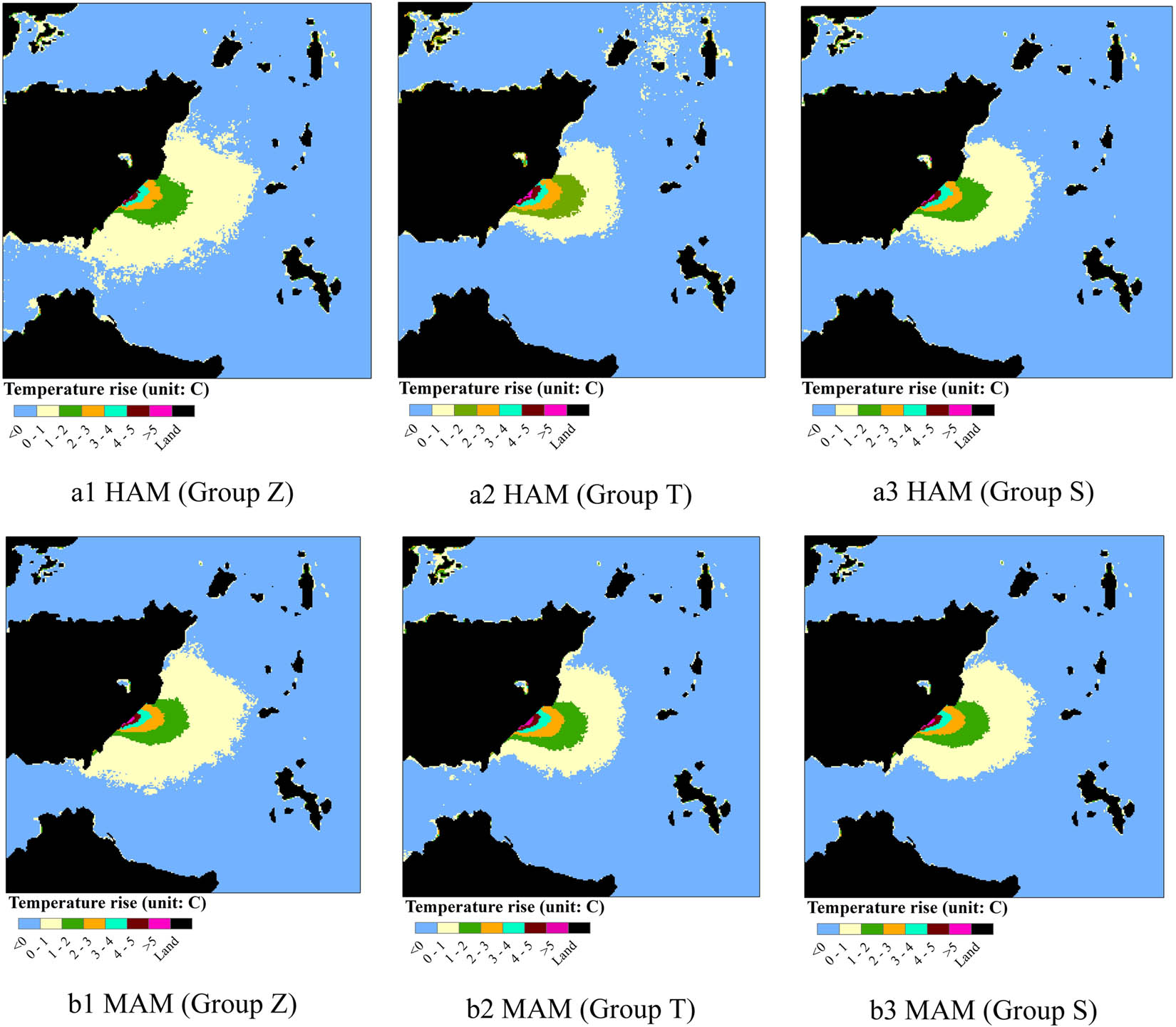
Temperature rise distribution maps extracted by HAM (as shown in a1, a2, a3) and MAM (as shown in b1, b2, b3) of Group Z, T, and S.

Three groups of SST were obtained by removing the data for some months from the 101 SST products. They were Group A (missing February, March, and November data), Group B (missing May, September, and October data), and Group C (missing January, April, and July data). The stability of the two methods was analyzed by comparing the extraction results of different groups, as shown in Figure 8. It can be seen that the temperature-rise distribution obtained by HAM has little change in the three groups. Meanwhile, the MAM results change greatly, mainly concentrated in the 0–1°C areas.

Figure 8

Temperature rise distribution maps extracted by HAM and MAM of Groups A, B, and C.

The percentages of pixels belonging to different temperature-rise grades across the whole water body were calculated to quantitatively compare the changes in the temperature-rise distributions of the three groups (Table 5). The smaller the standard deviation, the more stable the method. Table 5 shows that the standard deviations of the two methods are similar in temperature-rise classes 1–2, 2–3, 3–4, and 4–5°C, and are all <0.04. For the 0–1°C temperature rise, the standard deviation of MAM is 0.461, which is much greater than that of HAM. For all pixels >0°C, the standard deviation of MAM is 0.506 and that of HAM is 0.128. Therefore, overall, HAM has little dependence on samples and can also obtain more stable results when certain months are excluded.

Table 5

Pixel number percentages for different temperature-rise classes

	Missing months	0–1°C/%	1–2°C/%	2–3°C/%	3–4°C/%	4–5°C/%	>5°C/%	>0°C/%
MAM	2, 3, 11	3.031	0.483	0.151	0.061	0.025	0.008	3.759
	5, 9, 10	2.724	0.448	0.153	0.061	0.026	0.008	3.421
	1, 4, 7	2.214	0.415	0.146	0.063	0.027	0.010	2.874
	All data	2.027	0.396	0.139	0.057	0.025	0.007	2.652
	Mean	2.500	0.435	0.147	0.060	0.026	0.008	3.177
	Standard deviation	0.461	0.038	0.006	0.002	0.001	0.001	0.506
HAM	2, 3, 11	1.729	0.317	0.108	0.050	0.018	0.004	2.226
	5, 9, 10	1.716	0.359	0.099	0.055	0.022	0.004	2.256
	1, 4, 7	1.925	0.372	0.124	0.056	0.021	0.004	2.503
	All data	1.835	0.363	0.113	0.057	0.021	0.005	2.394
	Mean	1.801	0.353	0.111	0.054	0.021	0.004	2.345
	Standard deviation	0.098	0.024	0.010	0.003	0.002	0.001	0.128

5 Discussion

In the environmental impact assessment of the nuclear power plant, it is important to obtain the long-term stability impact area of the thermal discharge in a period of time. Most existing research studies using thermal infrared remote sensing methods are based on single or discrete data to obtain the variation trend and characteristics of the thermal discharge. Some scholars have proposed the temperature rise envelope method to extract the influence range of the nuclear plant cooling water from the perspective of long time series, but it cannot reflect the long-term impact area scientifically and has drawbacks in the application.

The concept of thermal discharge long-term impact area is introduced, and HAM is proposed to extract it based on SST products. Taking DNPS as a case study, first 101 scenes of TM/ETM+ remote sensing images from 2000 to 2013 were attained to get SST products using the single-channel thermal infrared inversion method, and the inverted SST was verified using the NR_2P products. Second, the annual cycle harmonic model was established to extract the RACPs, and differences between the reconstructed SST and original inverted SST were compared and analyzed to evaluate the model’s accuracy. Some factors, like cloud cover and tide, could affect the spatial distribution of the RACPs; thus, the influence of cloud cover and tide on RACPs was analyzed. Finally, taking the harmonic remainder and the mean image of the inverted SST products as the basic image, respectively, the HAM and MAM were applied to extract the temperature rise distribution maps of the thermal discharge impact area of different tides. By comparing the results of HAM and MAM, the following conclusions can be drawn.

An annual SST cycle harmonic model based on the SST time series was constructed. The mean difference between the modeled and original SST values ranged from −2.1 to 2.5°C, with a standard deviation range of 0 to 1°C. The model can describe the entire annual SST cycle and remove cloud effectively. This method provides new strategies for separating and restoring random noise information (e.g., cloud and fog) from periodic time series images.
The RACPs are affected by clouds and tides. As cloud cover increases, the harmonic remainder and amplitude decrease. Both have higher values during a rising tide than a falling tide due to the effect of water flow on thermal discharge diffusion.
The extraction results of the HAM and MAM are similar, and the later gives less noise when the input SST products are sufficient and distributed every month evenly. However, when the input SST products miss data for some months, temperature rise distribution obtained by the HAM changes little and the MAM shows the contrary. Although HAM introduces a small amount of noise during the process of cloud pixel recognition and compensation, it still obtains good results when several months of SST data are missing, showing that it has good robustness and great advantages in the assessment of thermal discharge impacts.

6 Conclusion

In the article, the HAM is proposed to extract the thermal discharge long-term impact area and acquire the temperature rise distribution of it, which not only provides a new way to acquire the thermal discharge influence area comprehensively over a period of time under particular situations (e.g., different tides, different generator units) but also makes it possible to calculate the acreage of temperature rise and evaluate the influence quantitatively. In addition to this, the thermal discharge long-term impact area could provide a basis for thermal discharge mixing zone establishing and precise pollution control. Compared with the existing remote sensing monitoring studies on thermal discharge, the HAM reduces the contingency of monitoring using single or discrete data, thus improving the stability and reliability of the result. Compared with the MAM, the HAM has less dependence on the input SST products and is more universal in application. However, the HAM is relatively complicated, and it takes a lot of time to collect and process long time series data. Therefore, how to improve the monitoring efficiency while ensuring accuracy is an important aspect of the development of nuclear power plant thermal discharge monitoring using remote sensing technology.

Abbreviations

HAM: Harmonic analysis method
MAM: Multi-year average method
DNPS: Daya Bay Nuclear Power Station

Acknowledgments

This research was supported by the Remote Sensing Geological Survey and Monitoring of the National Mine Environmental Restoration and Control Project (grant DD20190705) and the National Natural Science Foundation of China (grant 41501402).

Author contributions: Thanks are due to Yin Yaqiu from the Land Concolidation and Rehabilitation Center, Ministry of Natural Resources for the main research work, Yu Yang from the China Institute of Geo-Environment Monitoring for the technical guidance, Zhao Limin from the Aerospace Information Research Institute, Chinese Academy of Sciences, for providing and collating tidal observation data, Yang Hongyan from the Satellite Application Center for Ecology and Environment for providing important materials for thermal discharge assessment, Wang Jie and Yang Jinzhong from the China Aero Geophysical Survey and Remote Sensing Center for Natural Resources for assistance with data collection and processing.
Conflict of interest: Authors state no conflict of interest.

References

[1] Zhao A, Wang S, Zhao Y, Yuan J. Analysis of key issues in environmental impact assessment of thermal discharge from coastal nuclear power plant. Environ Impact Assess. 2015;37:57–60.10.1016/j.eiar.2016.05.002Suche in Google Scholar

[2] Masuda R. Tropical fishes vanished after the operation of a nuclear power plant was suspended in the Sea of Japan. PLoS One. 2020;15(5):e0232065.10.1371/journal.pone.0232065Suche in Google Scholar PubMed PubMed Central

[3] Wei X, Wang Y, Zhang K, Dang Y, Xiong X, Shang Z. Review of impact assessments of thermal discharges from power plants on aquatic biota. Chin J Ecol. 2018;39(2):1–10.Suche in Google Scholar

[4] Li K, Ma J, Huang L, Tan Y, Song X. Environmental drivers of temporal and spatial fluctuations of mesozooplankton community in Daya Bay, northern south China sea. J Ocean Univ China. 2021;20(4):1013–26.10.1007/s11802-021-4602-xSuche in Google Scholar

[5] Wang S, Chen F, Zhang W. Numerical investigation of temperature distribution of thermal discharge in a river-Type reservoir. Pol J Environ Stud. 2019;28(5):3909–17.10.15244/pjoes/99238Suche in Google Scholar

[6] Zeng Z, Luo Y, Chen Z, Tang J. Impact assessment of thermal discharge from the Kemen power plant based on field observation and numerical simulation. J Coast Res. 2020;104(sp1):1–11.10.2112/JCR-SI104-064.1Suche in Google Scholar

[7] Zhang YH, Li JG, Zhu L, Su XB, Yang HY. Optimization research on the ocean surface sampling and space interpolation method of thermal discharge monitoring. Mar Environ Sci. 2017;36(5):765–73.Suche in Google Scholar

[8] Zhu L, Zhao LM, Wang Q, Zhang AL, Wu CQ, Li JG, et al. Monitoring the thermal plume from coastal nuclear power plant using satellite remote sensing data: modeling and validation. Spectrosc Spectr Anal. 2014;34(11):3079–84.Suche in Google Scholar

[9] Ai B, Wen Z, Jiang Y, Gao S, Lv G. Sea surface temperature inversion model for infrared remote sensing images based on deep neural network. Infrared Phys Technol. 2019;99:231–9.10.1016/j.infrared.2019.04.022Suche in Google Scholar

[10] Meng X, Cheng J. Estimating land and sea surface temperature from cross-calibrated Chinese Gaofen-5 thermal infrared data using split-window algorithm. IEEE Geosci Remote Sens Lett. 2020;17(3):509–13.10.1109/LGRS.2019.2921863Suche in Google Scholar

[11] Xie X. Determination of inland river constant water level in artificial island based on tidal influence. Port Waterw Eng. 2021;(11):8–12.Suche in Google Scholar

[12] Yavari SM, Qaderi F. Determination of thermal pollution of water resources caused by Neka power plant through processing satellite imagery. Environ Dev Sustainability. 2020;22(3):1953–75.10.1007/s10668-018-0272-2Suche in Google Scholar

[13] Nie P, Wu H, Xu J, Wei L, Ni L. Thermal pollution monitoring of Tianwan nuclear power plant for the past 20 years based on Landsat remote sensed data. IEEE J Sel Top Appl Earth Obs Remote Sens. 2021;14:6146–55.10.1109/JSTARS.2021.3088529Suche in Google Scholar

[14] Roy P, Rao IN, Martha TR, Kumar KV. Discharge water temperature assessment of thermal power plant using remote sensing techniques. Energy Geosci. 2022;3(2):172–81.10.1016/j.engeos.2021.06.006Suche in Google Scholar

[15] Wang R, Yang H, Zhu L, Chen Y. Application of temperature rise envelope in monitoring of nuclear power plant cooling water temperature. Adm Tech Environ Monit. 2020;32(1):4.Suche in Google Scholar

[16] Malamiri G, Zare H, Rousta I, Olafsson H, Mushore TD. Comparison of harmonic analysis of time series (HANTS) and multi-singular spectrum analysis (M-SSA) in reconstruction of long-gap Missing data in NDVI time series. Remote Sens. 2020;12(17):2747.10.3390/rs12172747Suche in Google Scholar

[17] Song DM, Lin Z, Shan XJ, Yuan Y, Cui JY, Shao HM, et al. A study on the algorithm for extracting earthquake thermal infrared anomalies based on the yearly trend of LST. Seismol Geol. 2016;38:680–95.Suche in Google Scholar

[18] Ahmed T, Singh D. Probability density functions based classification of MODIS NDVI time series data and monitoring of vegetation growth cycle. Adv Space Res. 2020;66(4):873–86.10.1016/j.asr.2020.05.004Suche in Google Scholar

[19] Bechtel B. Robustness of annual cycle parameters to characterize the urban thermal landscapes. IEEE Geosci Remote Sens Lett. 2012;9(5):876–80.10.1109/LGRS.2012.2185034Suche in Google Scholar

[20] Fu P, Weng Q. Variability in annual temperature cycle in the urban areas of the United States as revealed by MODIS imagery. ISPRS J Photogramm Remote Sens. 2018;146(dec):65–73.10.1016/j.isprsjprs.2018.09.003Suche in Google Scholar

[21] Tian G, Liu Q, Chen L. Thermal remote sensing. Beijing: Electronic Industry Press; 2014. p. 172–4.Suche in Google Scholar

[22] Feng C, Xiaofeng Z, Yuan Q. Single-channel method based on temporal and spatial information for retrieving land surface temperature from remote sensing data. J Remote Sens. 2014;18(3):657–72.10.11834/jrs.20143167Suche in Google Scholar

[23] Todorova M, Grozeva N, Takuchev NP, Ivanova D, Boneva V. Vegetation in Bulgaria according to data from satellite observations and NASA models. IOP Conference Series Materials Science and Engineering. Vol. 1031, Issue 1, 2021. p. 012083.10.1088/1757-899X/1031/1/012083Suche in Google Scholar

[24] Zeng L, Wardlow BD, Hu S, Zhang X, Wu W. A novel strategy to reconstruct NDVI time-series with high temporal resolution from MODIS multi-temporal composite products. Remote Sens. 2021;13(7):1397.10.3390/rs13071397Suche in Google Scholar

[25] Zhou J, Jia L, Menenti M, Liu X. Optimal estimate of global biome-specific parameter settings to reconstruct NDVI time series with the harmonic analysis of time series (HANTS) method. Remote Sens. 2021;13(21):217–28.10.3390/rs13214251Suche in Google Scholar

[26] Willmott CJ, Robeson SM, Matsuura K. Short communication a refined index of model performance. R Meteorol Soc. 2012;32:2088–94.10.1002/joc.2419Suche in Google Scholar

Received: 2021-06-17

Revised: 2022-11-10

Accepted: 2023-03-03

Published Online: 2023-04-06

This work is licensed under the Creative Commons Attribution 4.0 International License.

Artikel in diesem Heft

https://doi.org/10.1515/geo-2022-0471

Schlagwörter für diesen Artikel

thermal infrared remote sensing; harmonic analysis method; the robust annual cycle parameters; thermal discharge long-term impact area; SST; Daya Bay Nuclear Power Station; TM/ETM+

Creative Commons

BY 4.0