Interpretation of aeromagnetic and remote sensing data of Auchi and Idah sheets of the Benin-arm Anambra basin: Implication of mineral resources
-
Olubukola A. Oni
 ,
Sodiq A. Alimi
,
Sodiq A. Alimi

Abstract
The need for mineral resources for economic development is key in both developing and developed countries. However, miners usually resort to random excavation of mineral deposits without proper investigation to identify structures of interest in target areas. This usually leads to land depletion and abandonment. The aim of this study is to assess the mineral potential in part of the Benin-arm of the Anambra basin by investigating the geophysical characteristics of the area using remote sensing and aeromagnetic data. Surface and subsurface regional structures, including faults and zones of mineralisation, were mapped by integrating aeromagnetic and remote sensing data. The mineral bearing zones that show high prospects of mineral deposits in the region were identified. The rose diagram revealed that the surface lineaments are aligned in the NW–SE, N–S, NE–SW, E–W, NNE–SSW, ENE–WSW, and ESE–WNW directions. The orientations of the subsurface lineaments are aligned mostly in the NE–SW, N–S, and E–W directions. The magnetic intensity ranged between −431.38 and 399.82 nT, while reduction-to-pole magnetic intensity ranged from –416 to 664.45 nT. The first vertical derivative showed magnetic intensity which ranged from –0.5863 to 0.9060 nT/km2. The total horizontal derivative magnetic intensity ranged from –0.00031 to 0.762691 nT/km2, while the analytic signal showed magnetic intensity ranging from 14.0664 to 394,607.3438 nT/cm2. The windowed Euler deconvolution depth to magnetic source showed depth range of <20 to 2,000 m. Many of the features delineated in the study area were characterised by shallow magnetic source depths (<500 m); this is a common characteristic of basement complex terrains. Deeper magnetic source depths (>1,000 m) were observed in the sedimentary terrain. Mineral exploration should be focused in areas with high lineament concentration, as lineaments are potential conduits for economic minerals deposition.
1 Introduction
In both developing and developed countries, the need for mineral resources for economic growth is crucial. As a result, more attention is being placed on harnessing mineral resources aside from oil and gas to support the recovery of the country’s economic growth [1,2,3,4]. In many developing countries, including Nigeria, the mining of mineral resources is of paramount importance [3]. Nigeria is endowed with abundant natural resources that have added enormously to the socio-economic benefits and wealth of the country [5]. However, the greatest difficulty in the development of large-scale mining is the lack of a comprehensive understanding of the geophysical characteristics of the region. Thus, miners sometimes result in random excavation of mines in their effort to locate primary deposits. This exposes several non-mineralised areas that would have been used for agricultural purposes to large scale land depletion and abandonment. Consequently, significant and economic mining activities require a comprehensive understanding of the geophysical characteristics of the region. Although mineral resources are essential sources of wealth for a country and need to be explored, mined, and processed before they can be of value, these processes are capital intensive. Extensive geological information is required for effective exploration; this would reduce the cost of exploration. This extensive analysis requires the use of geophysical methods. Therefore, this study is an assessment of the mineral resource potential in part of the Benin-arm of the Anambra basin using aeromagnetic and remote sensing data.
1.1 Detailed geology of the study area
The study area covers Auchi and Idah of the Benin-arm of the Anambra basin (Figures 1 and 2). The area mostly covers the northern part of Edo state, extending into the southern part of Kogi state, Nigeria. The area lies within the geographical coordinates of latitude 7°0′0″ and 7°30′00″ North and longitude 6°0′0″ and 6°60′0″ East. The climate is tropical and humid; the temperature varies from 42°C in February to 23°C in July. The area is marked by two distinct seasons: the dry and rainy seasons. The dry season spans between late September and early April, while the rainy season is between late April and early September. The Anambra Basin is one of Nigeria’s Cretaceous sedimentary basins [6,7]. The basin is bounded by the Niger Delta Hinge Line on the south–western flank, the Benue Flank in the north–west, and the Abakaliki fold belt in the south–east [6]. The southern frontier of the basin overlaps with the northern frontier of the Niger Delta basin [8].

Map of the study area (Auchi and Idah).
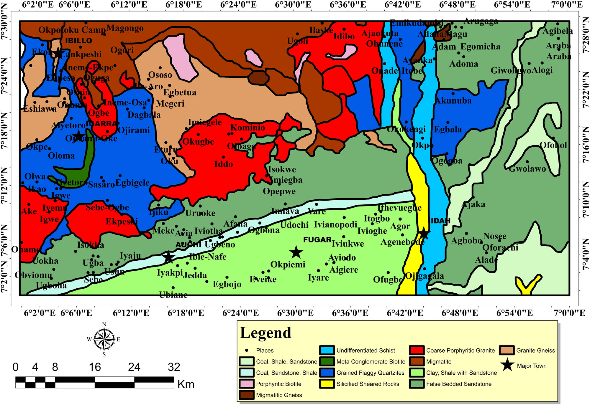
Geological map of the study area.
The basin is coarsely triangular in shape, which covers an approximate area of 40,000 km2 in which the sediment thickness aggregates southwards to a maximum thickness of 12,000 m in the central fragment of the Niger Delta region [6,8]. The Anambra basin stretches from the southern part of the confluence of the west of the River Niger and Benue through terrains like Asaba, Okene, Auchi, Agbo, and to the east of the river Awka, Idah, Onitsha, Nsukka, and Anyangba area. The Udu-Idah cliff slopes slightly in the southwest direction into the flood plain of the River Niger and across to the west at an elevation of about 300 m [9]. The basin is mainly drained by the Anambra River and its main tributaries, the Mamu and Adada [9].
2 Methods
The methods deployed in this study include the aeromagnetic and remote sensing methods. The raw aeromagnetic data of sub-nanotesla resolution scale was obtained from the Nigerian Geological Survey Agency.
The Landsat8 image (Path/Row-191/054) resolution of 30 m was provided by the United States Geological Survey in collaboration with the National Aeronautics and Space Administration. Using the Operational Land Imager sensor, the Landsat image was captured on February 4, 2014, at 10:03:33 am with the solar elevation angle at 52.14° and the azimuth of the sun at 130.8°.
2.1 Aeromagnetic data processing
To process the aeromagnetic data, two databases were created using the magnetic data processing software by Oasis Montaj Geosoftware 7.0. The data processing consists of four procedures, which are gridding, determination of the residual magnetic field by subtracting IGRF from total magnetic data measured from the field, micro-levelling of the whole dataset to eliminate any form of errors [10,11], and integration of the different windows for each different type of data using different filtering techniques expressed in equations (1)–(3).
Interpretation was carried out by inspecting the total magnetic field. The residual map was generated after the removal of regional effects from the total magnetic intensity using the Butterworth low-pass filtering method. Butterworth helped in simplifying the filter by using a normalised low-pass polynomial. The residual anomaly maps are derived using polynomial fitting to desirable degrees. Polynomial fitting degrees 1 and 2 were used to generate residual anomaly maps and to investigate how the degree of polynomial fitting affects the appearance of the maps. The equation used in the algorithm for the separation of the regional field is expressed as follows:
where
RTP algorithm was applied to the total magnetic anomaly because the data were acquired closer to the magnetic latitude. The RTP map was produced by applying RTP filter on the RMI map using Fast Fourier Transform (FFT). The RTP operation in wave number domain can be represented as follows:
where
The parameters involved include an inclination value of −11.27 and a declination value of −1.18. An amplitude correction value of 60 was also applied to reduce latitudinal effects because the survey was carried out in an area close to the equator, hence RTP at low latitude.
The RTP grid data were subjected to a first vertical derivative (FVD) filter. The FVD filter allows small and large amplitude responses to be more equally represented. The FVD grid helps enhance linear features in the area. Vertical derivative filters are generally applied to gridded data using FFT filters. These maps were produced by the application of derivative filters on the RTP map of the area of study using FFT. An upward continuation value of 200 was also applied to the filter in order to reduce the influence of signatures that may be due to manmade features. Different vertical derivatives of the magnetic fields can be measured through multiplication of the field’s amplitude spectra by a factor in the form as follows:
where
The analytic signal behaves like the RTP filter. It actually takes the magnitude of the square root of the vertical and horizontal components of the magnetic responses [13]. This processing enhancement was used in mapping the edges of the permanently magnetised sources and for centering anomalies over their causative bodies in areas of low magnetic latitude but does not depend on the direction of magnetisation. The analytic signal map was created via the application of an analytic signal filter on the RMI map of the area of study. The extension of the Geosoft Oasis Montaj’s depth to basement, which defines the location (distance along the profile and depth), dip (orientation), and intensity (susceptibility) of magnetic source bodies for magnetic profiles, was used in an attempt to measure the depth to basement of the magnetic bodies in the study area. In calculating the depth of the magnetic anomaly, the Euler deconvolution function, which makes use of both the horizontal and vertical derivatives, was employed.
The Euler deconvolution function assumes that the source body is either a dyke or contact of limitless depth and employs the least-square method in a series of shifting the profile windows to solve for source body parameters [14]. Solutions deduced from total field profile are referred to as “Dyke” solutions, while solutions resulting from horizontal gradient are referred to as “Contact” solutions. Euler deconvolution algorithm was used for the location and depth determination of causative anomalous bodies from gridded aeromagnetic data. The 1.0 and 2.0 values of the structural index (N) were used based on individual dykes and sills models of the source [15]. Through the application of the window method, the solutions derived were further refined to eliminate ambiguity. This was accomplished by limiting the solutions obtained from Euler deconvolution to a maximum tolerance depth of 10% while rejecting the uncertainty in depth (
2.2 Landsat 8 processing
The image processing software Environment for Visualising Images (ENVI) version 5.1 was used for processing the remote sensing data. The remote sensing data were interpreted using ArcGIS, Rockware, PCI Geomatic software, Rockworks, and GeoRose software. Atmospheric correction was applied to the Landsat8 scenes using the Fast Line-of-sight Atmospheric Analysis of Spectral Hypercube (FLAASH) algorithm [16]. The FLAASH algorithm was implemented using the Sub-Arctic Summer atmospheric and maritime aerosol models [13]. During the atmospheric correction, raw radiance data from the imaging spectrometer were re-scaled to reflectance data.
Colour composite images were produced based on known spectral properties of rocks and alteration minerals in relation to the selected spectral bands. Bands 4, 3, and 2 were used to produce true colour composite, while bands 5, 4, and 1 were used to produce false colour composite images of the study area for lithological mapping. Both the true and false colour maps were produced by importing individual 8-bit greyscale surface reflectance bands of the Landsat8 data into the ENVI workspace. This was applied after the Landsat8 data for the area had been processed and corrected using ENVI and ArcGIS software. Band ratio indices were developed and implemented to Landsat8 spectral bands for mapping poorly exposed lithological units, geological structures, and mineral alteration in the study area. Spectral-band ratio indices were used to map the spectral signatures of iron oxide/hydroxide minerals, the OH– and Fe, and Mg–O–H bearing lithological units within the area of study. The surface and subsurface lineaments were merged in ArcGIS to get a detailed understanding of the lineament structure or lineament pattern of the research area. Two band ratios were formed based on the laboratory spectral of minerals for mapping the abundance of iron oxide/hydroxide minerals in rocks using the Landsat8 bands [17,18]. Goethite, jarosite, hematite, and limonite are typically heavily absorbed into visible and near-infrared (0.4–1.1 μm), coinciding with Landsat8 bands 2, 3, 4, and 5, and high reflectance into short wave infrared (SWIR) (1.56–1.70 μm) coinciding with Landsat8 band 6 [19]. Therefore, band ratio of 4/2 was used to map iron oxide mineral groups. The Landsat8 SWIR bands were used to detect hydroxyl-bearing (Al–OH and Fe, Mg–OH) groups within the study area. Clay minerals contain 2.1–2.4 μm spectral absorption features and 1.55–1.75 μm reflectance, coinciding with Landsat8 band 7 (2.11–2.29 μm) and band 6 (1.57–1.65 μm) [19]. Therefore, ratio 6/7 was used to map the hydroxyl-bearing mineral group in this study. For the ferromagnesium (Fe, Mg–OH) group of minerals, bands 5 and 6 of Landsat8 were used due to the group’s high absorption feature in band 5, and low absorption characteristics in band 6.
For a detailed structural and lithological mapping of the study area, surface structures were extracted from processed Landsat8 data of the area using the automatic lineament extraction tool in PCI Geomatica. The lineament density map was produced by combining both the surface and subsurface lineaments and calculating their densities using the line density tool. The surface and subsurface lineaments were merged in ArcGIS to aid a detailed understanding of lineament structure or lineament pattern in the study area.
3 Results
Figures 3 and 4 show the true and false colour composite maps of the area, respectively. The vegetation area appears as dark green on the true composite map, while the false composite map appears red. Human settlements appear light brown on both maps while the major river, which appear white on the true map, appear with a shade of cyan and white colouration on the false map. Areas with different geological or topographical settings are mostly seen in the upper western part of the area; these areas are mostly underlain by basement complex rocks. Igarra’s granite plutons of Somorika and Ojirami appear dark brown, while granite gneiss and migmatitic terrains appear brown. The eastern and southeastern parts of the study area are underlain with sedimentary rocks, which include sandstone and shale. These rocks underlie the relatively flat surface and cannot be easily identified in the true colour composite image on a regional scale. Schist and migmatite in the Ugoli and Ajaokuta areas show clearly on the false colour composite map compared to the true colour composite map. Figure 5 shows areas with blue pixels in a grey shade for easy identification; the bright coloured areas represent high reflectance of ratio 6/7. Within the study area, carbonate rocks such as marble are present, and alteration products of such rocks include clay minerals. The green pixels represent areas with ferrous iron-bearing minerals such as olivine, pyroxene, and amphiboles (Figure 5), rocks such as schist and metaconglomerate in the study area host these minerals. The red pixels represent areas dominated by ferric-bearing minerals such as goethite, hematite, and jarosite (Figure 5). Figure 6 shows a greyscale map of band four divided by band two (4/2) for iron oxide alteration mapping. Figure 7 shows the greyscale map of band five divided by band six (5/6) for Fe and Mg–OH bearing lithological units, and Figure 8 shows the greyscale map of band six divided by seven (6/7) showing areas where OH-bearing clay alterations are present in the study area. Figure 5 shows the band ratio map of the area of study. Band ratios of 4/2, 6/7, and 5/6 boost minerals such as clay (pyllosilicates), ferrous, and iron oxides, respectively [20]. The colour composite image of these band ratios can be used to identify basement complex rocks such as granite, gneiss, basic igneous rocks, and arkose in the study area. Clay/kaolinite can be obtained from the weathering of feldspar-bearing arkose, gneiss, and granite; most schist and sedimentary rocks in the study area contain clay-bearing soils. Biotite bearing quartzite, gneiss, and granite can easily weather into iron oxide. Iron oxide alterations appear to be the most dominant form of alteration in the study area; this may be due to the constant interaction between exposed rocks and weathering agents such as wind and water.
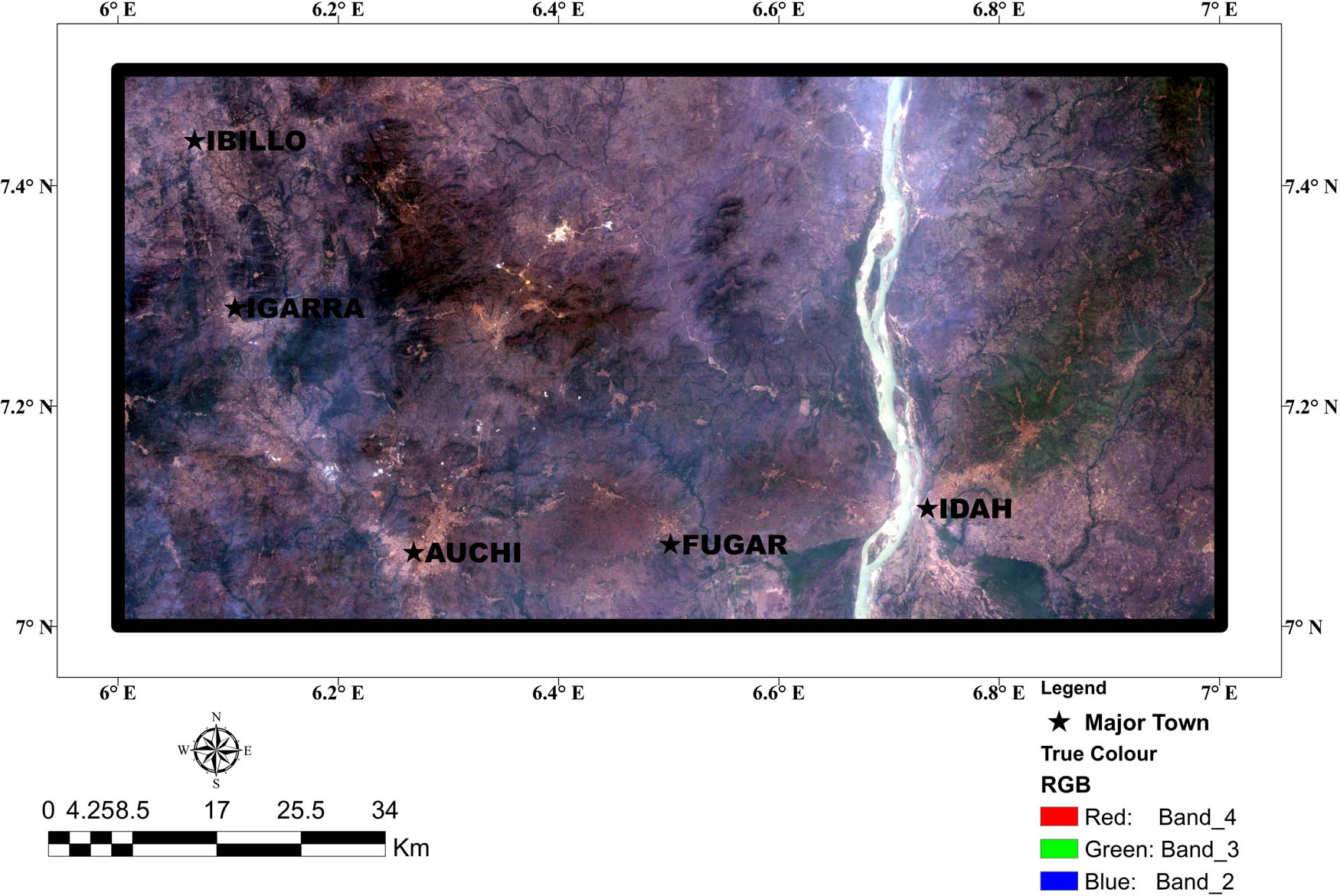
True colour composite (bands 4, 3, and 2) map of the study area.

False colour composite (bands 5, 4, and 3) map of the study area.

Band ratio map of the study area.

Ratio 4/2 (ferric-ion bearing) map of the area of study.
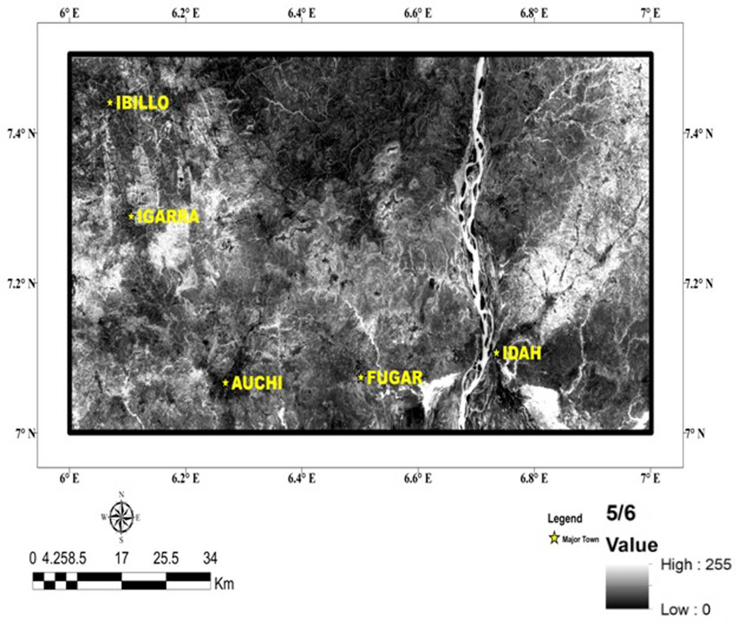
Ratio 5/6 (ferrous-ion bearing) map of the area of study.

Ratio 6/7 (OH bearing) map of the area of study.
Figure 9 shows extracted surface lineaments in the study area. The displayed lineaments represent geologic structures such as faults, joint-sets, fractures, and lithologic boundaries in the study area. In both the sedimentary and basement complex terrains, minerals are believed to be structurally controlled and the ability to identify these structures provides more information towards preparation of mineral activities. Therefore, the various surface linear features such as faults, joints, fractures, foliations, and river channels that are obvious on the surface were carefully mapped out. It can be seen that surface lineaments are well dispersed within the research area. Both the basement and sedimentary terrains show surface lineaments.

Surface lineaments present in the area of study.
Figure 10 shows the orientation of surface lineaments within the study area. The lineaments are aligned in the NW–SE, N–S, NE–SW, E–W, NNE–SSW, ENE–WSW, and ESE–WNW with a dominant direction towards NNW–SSE, which is similar to the orientations that have been reported earlier [21,22]. Also, the study by Ogbe et al. [21] showed that joints within Igarra and environs trend in the NE–SW to E–W direction. Ajigo et al. [22] also reported NNW–SSE and ENE–WSW as the dominant directions for both foliations and lineaments in the Ibillo-Okene area.

Plot of the general bearing of the surface lineaments.
4 Aeromagnetic results
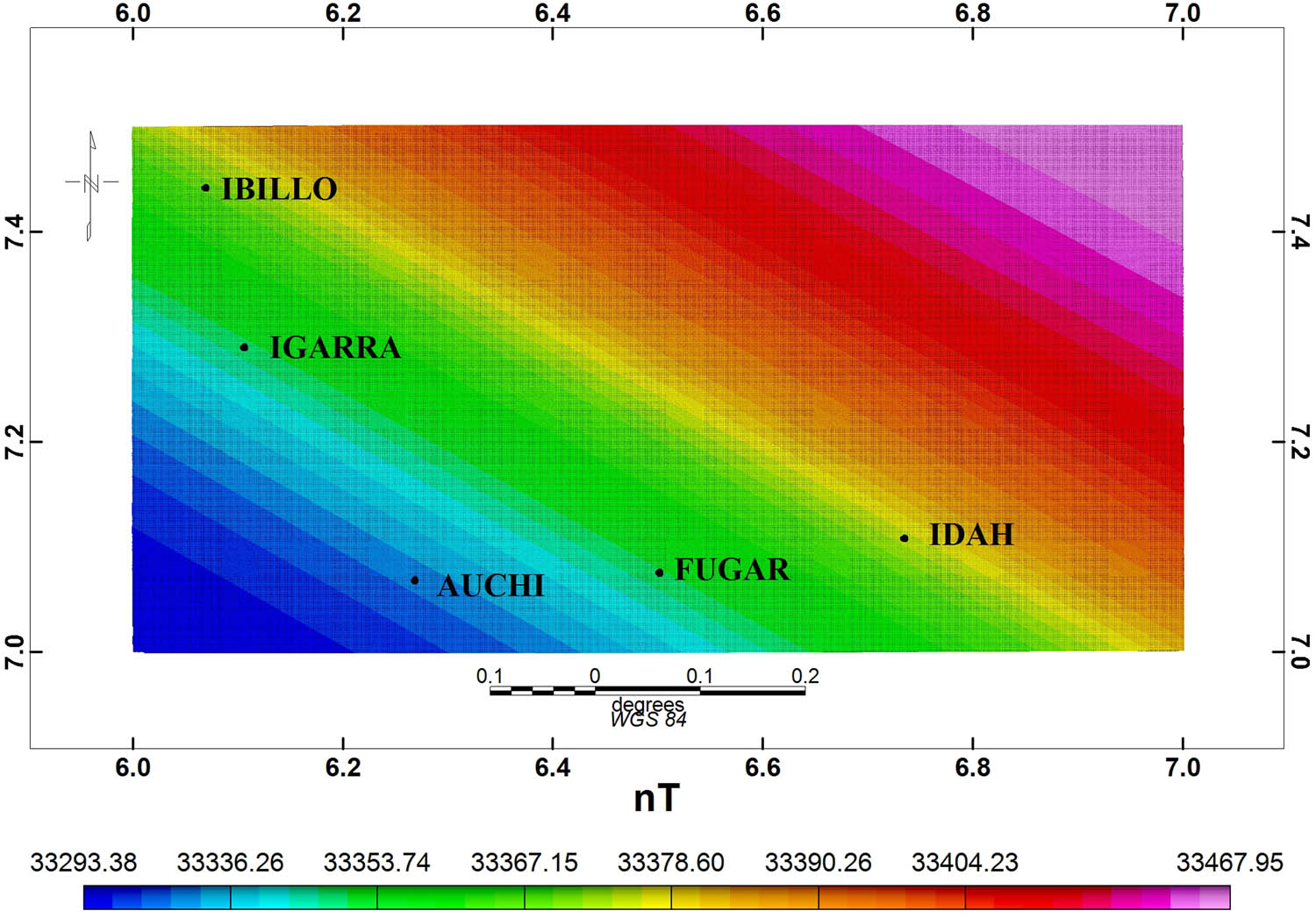
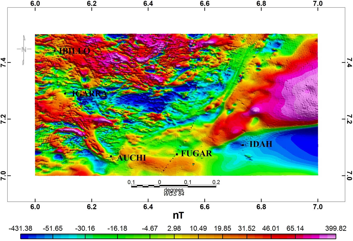
Figure 11 shows the total magnetic intensity map, Figure 12 shows the regional map, and Figure 13 shows the RMI map. The high magnetic intensity zones fall within the basement complex terrain with rocks that are rich in magnetic minerals. Examples of these rocks include basic igneous and metamorphic rocks such as schist, gneiss, dolerite, migmatite, granodiorite, and basalt. The low magnetic intensity values originate from the sedimentary areas covered by materials with low magnetic minerals. Such materials include shale, limestone, sandstone, mudstone, and alluvial sands. Magnetic intensity values within the study area ranged between −431.38 nT for magnetic low and 399.82 nT for magnetic high.

Total magnetic map of the study area.
Regional map of the study area.
RMI map of the study area.
Figure 14 shows the RTP map of the study area. The RTP map showed the magnetic intensity ranging from −416 to 664.45 nT. The sedimentary terrain in the eastern and southern parts of the study area shows low to moderate magnetic intensities, while the basement terrain in the western and north-western parts of the study area displays high magnetic intensities. Schists, migmatite, and gneiss are known to be rich in magnetic minerals compared to sandstone, mudstone, shale, and limestone in the area. Figure 14 shows a clear and distinct difference between the basement and sedimentary terrain. The sedimentary terrain appears smooth while the basement terrain appears rough. This is due to the geology of the area, the formation of rocks and the deformation that the rocks in the area have gone through.

RTP (at low latitude) map of the study area.
Figure 15 shows the FVD map of the area of study, while Figure 16 is the total horizontal derivative map of the study area. Both Figures 15 and 16 show subsurface lineaments such as faults present in the study area. It can be shown that the majority of the subsurface lineament appears in the basement terrain, while few of these lineaments are present in the sedimentary terrain. Figure 15 shows clearly that the complexity of structures within the basement terrain areas is a reflection of the various cycles of deformation that these rocks have undergone. The structures within the sedimentary terrains are dykes that have intruded into the sedimentary basins. A clear visualisation of the extracted lineaments, lithological boundaries, and geological structures such as folds is shown in Figure 17. Figure 18 shows the orientation of the subsurface structure, which aligns mostly in the NE–SW, N–S, and E–W directions. Figure 19 shows the lineament density map, whose density values range from 0 to 1.82. This map shows areas in which lineaments are concentrated. From the lineament density map, areas with high lineament concentration appear in orange colouration with a lineament value ranging from 1.01 to 1.82, while areas with moderate lineament concentration appear in yellow with a lineament value ranging from 0.32 to 0.6. Areas with low lineament concentration appear as areas with greenish colouration, with lineament values ranging from 0 to 0.12. Mineral exploration activity should be focused on these high lineament concentration areas due to the fact that lineaments serve as conduits of economic mineral deposits in rocks.

FVD map of the study area.

Total horizontal derivative map of the study area.
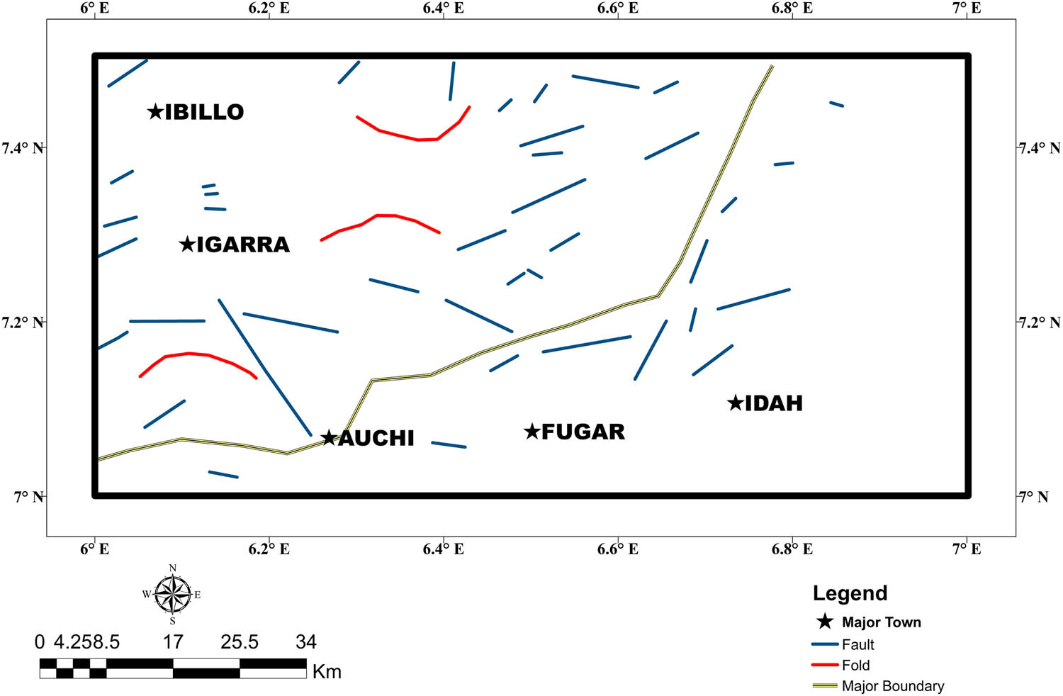
Vectorised subsurface lineaments of the area of study.

Plot of the general bearing of the subsurface lineaments.

Lineament density map of the study area.
The analytic signal map of the study area is shown in Figure 20. The analytical map showed magnetic intensity ranging from 14.0664 to 394607.3438 nT/cm2. It indicates clearly the sources of the magnetic anomalies. The igneous and metamorphic rocks in the basement terrain are the sources of the magnetic anomalies in the area of study. On the other hand, the sedimentary terrain shows low magnetic intensity signatures except in areas where dykes exist.
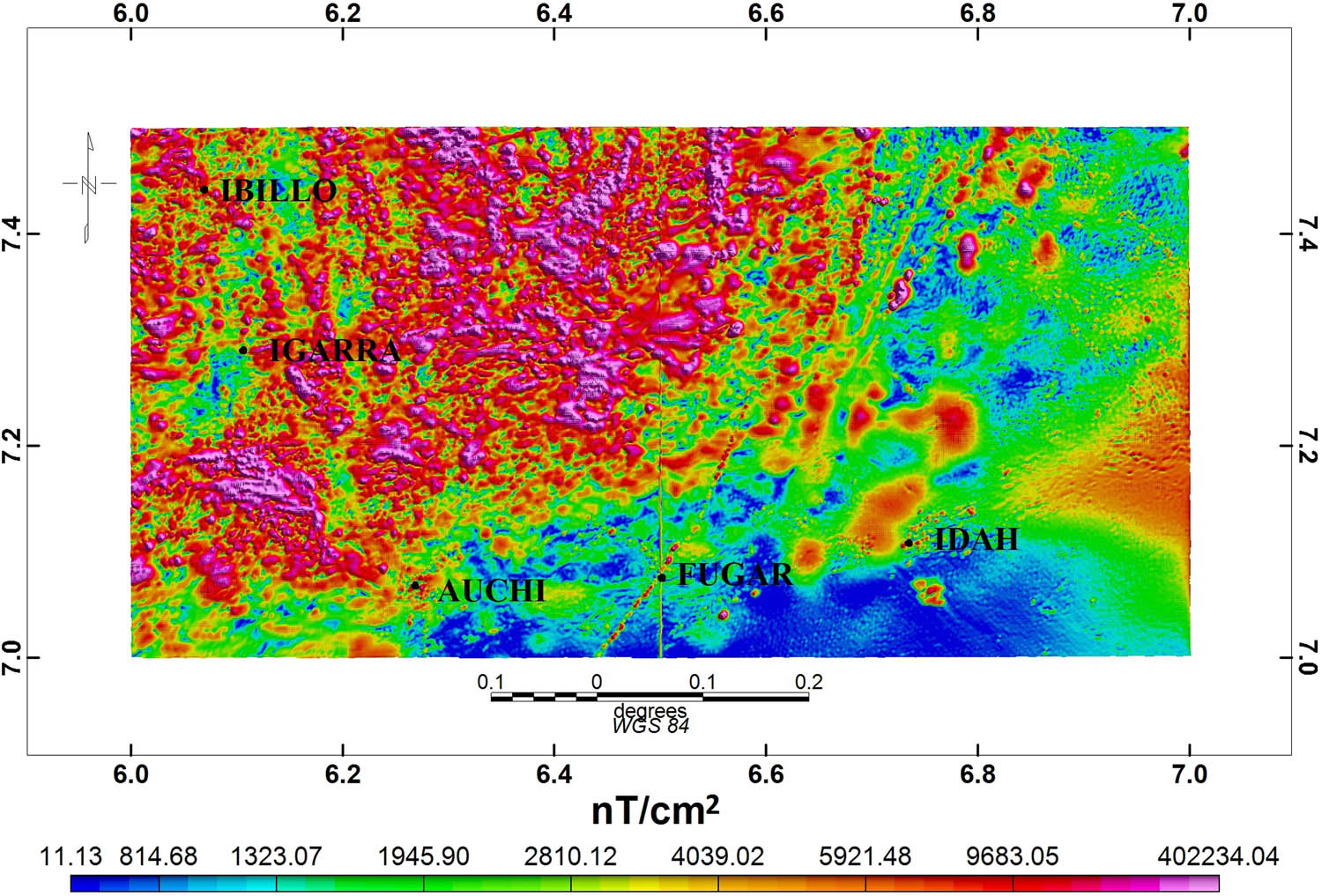
Analytical signal map of the study area.
Various Euler depths of 100, 500, 1000, and 2,000 m calculated for the study area are shown in Figures 21–24. It can be observed that shallow magnetic depths are common in the basement complex terrains, while deeper depths are seen in the sedimentary terrain. This is to be expected as the bedrock in the basement complex terrain is only overlain by a relatively thin overburden, while piles of sediment over the basement (bedrock) in the sedimentary area are very thick in comparison. Previous studies [23,24,25] carried out in the Anambra basin agreed with the results of the present study and indicated that shallow depth sources are common in basement complexes, while deeper depth sources are observed in sedimentary terrains.

Windowed Euler deconvolution depth to magnetic source (100 m).

Windowed Euler deconvolution depth to magnetic source (500 m).
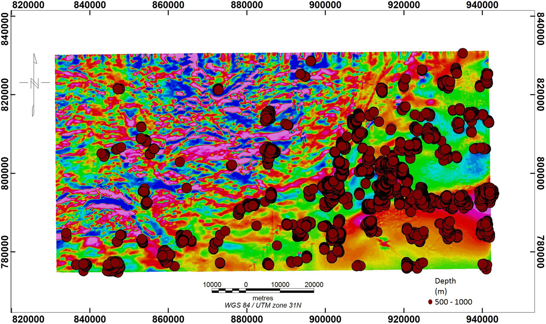
Windowed Euler deconvolution depth to magnetic source (1,000 m).
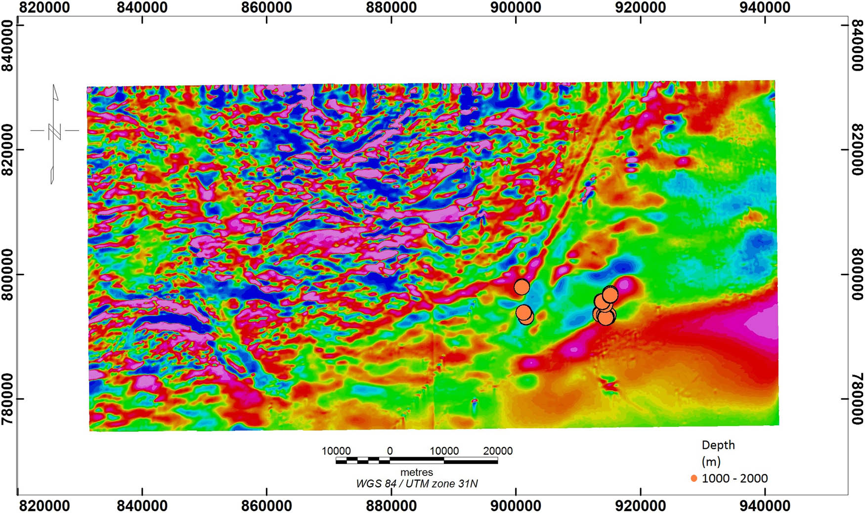
Windowed Euler deconvolution depth to magnetic source (2,000 m).
5 Discussion
5.1 Implication for mineral resources
This aim of this study was mapping the lithology and structure of sheets 266 and 267. The objectives of the study are to map out the various lithologies and structures present in the area and assess their potential for mineral exploration. Mineralised pegmatite vein, which are often easily weathered due to the effect of water on feldspar [26], appear to produce clay-like signatures on the band ratio maps. The ability to find such areas helps in easily detecting veins, which can play a major role to host minerals of economic benefit. Also, gold mineralisation has often been discovered in areas within the iron oxide alteration zones [26]. These outcomes provide focus on knowledgeable objectives for better preparation before exploration, rather than random excavation that can lead to waste of resources, time, and money. The lineament map shows areas of high, moderate, and low lineament density. The presence of lineaments shows that the area has the potential to host mineralisation because lineaments can potentially serve as conduits through which hydrothermal alteration can occur. The result from the rose diagram revealed that the surface lineaments are aligned in the NW–SE, N–S, NE–SW, E–W, NNE–SSW, ENE–WSW, and ESE–WNW. The orientations of the subsurface lineaments align mostly in the NE–SW, N–S, and E–W directions, which agrees with the previous studies [21,22].
However, aeromagnetic method results showed that the magnetic intensity values ranged between −431.38 nT for magnetic low and 399.82 nT for magnetic high, with RTP map magnetic intensity ranging from −416.45 to 664.45 nT. The FVD map showed magnetic intensity values which ranged from −0.5863 to 0.9060 nT/km2. The total horizontal derivative map intensity ranged from −0.00031 to 0.762691 nT/km2 while the analytical map showed magnetic intensity ranging from −14.0664 to 394607.3438 nT/cm2. The windowed Euler deconvolution depth to magnetic source showed depth range of <20 to 2,000 m. The results also show the major lithological boundary between the basement and sedimentary rocks in the area. Various structures were deduced from the first, second, and total vertical and horizontal derivative maps of the area. These structures are a product of tectonism and their various orientations agree with the findings from previous research in the area. For example, areas characterised by iron oxide alteration are the most suitable for gold exploration due to various hydrothermally altered structures, which is in line with the works of Ejepu et al. [26]. Also, clay alteration zones sometimes are regions where mineralized pegmatites are weathered, which agrees with the work of Obaje [27]. Based on the findings of this research, it is concluded that the area of study has huge mineral exploration potential and it is not surprising that various deposits have been recorded already, which include iron ore, marble, coal, and kaolinite.
Acknowledgement
This is to appreciate Covenant University Centre for Research Innovation and Discovery (CUCRID) and Covenant University as a whole for their financial support towards this study.
-
Author contributions: O.A.O. developed the concept, methodology, and worked on formal analysis, resources, data curation, writing – original draft, visualisation, and writing – review and editing. H.O.B. worked on methodology and review. S.A.A. worked on data curation and methodology. A.P.A. worked on the grammatical errors.
-
Conflict of interest: The authors state no conflict of interest.
References
[1] Adagunodo TA, Sunmonu LA, Adetunji AA. An overview of magnetic method in mineral exploration. J Glob Ecol Environ. 2015;3(1):13–28.Suche in Google Scholar
[2] Olasunkanmi NK, Sunmonu LA, Adabanija MA, Oladejo PO. Interpretation of high resolution aeromagnetic data for mineral prospect in Igbeti-Moro area, southwestern Nigeria. IOP Conf Ser Earth Environ Sci. 2018;173(1):1–9. 10.1088/1755-1315/173/1/012033.Suche in Google Scholar
[3] Amadikwa LO, Selemo AI, Obioha YE, Okorie OJ. Application of aeromagnetic data for mineral exploration in Igarra and environs, southwestern Nigeria. Int J Adv Acad Res. 2019;5(10):10–25.Suche in Google Scholar
[4] Obiora DN, Okorie AC. Spectral analysis and modeling of magnetic anomalies in part of northern Anambra basin, Nigeria. Environ Res J. 2020;14(3):84–96.Suche in Google Scholar
[5] Okorie AC, Obiora DN, Igwe E. Geophysical study of Ubiaja and Illushi area in northern Anambra basin, Nigeria, using combined interpretation methods of aeromagnetic data. Model Earth Syst Environ. 2019;5(3):1071–82. 10.1007/s40808-019-00592-0.Suche in Google Scholar
[6] Asadu AN, Ibe KA. Petroleum geology of outcropping sediments along Imiegba road in etsako east local government area of Edo state, southern Anambra basin flank, Nigeria: inference from sedimentology and organic geochemistry. J Geogr Environ Earth Sci Int. 2017;10(3):1–10. 10.9734/JGEESI/2017/33891.Suche in Google Scholar
[7] Onu KF. The Southern Benue trough and Anambra Basin, Southeastern Nigeria: A stratigraphic review. J Geogr Environ Earth Sci Int. 2017;12(2):1–16. 10.9734/JGEESI/2017/30416.Suche in Google Scholar
[8] Igbinigie N, Akenzua A. Palynological studies of maastrichtian to Paleocene sediments exposed at Okpekpe, western flank of Anambra basin, Edo state, Nigeria. J Appl Sci Environ Manag. 2018;22(10):1563–6. 10.4314/jasem.v22i10.05.Suche in Google Scholar
[9] Yusuf I, Ogundele JO, Odejobi Y, Auwal HI. Geophysical investigation of loss of circulation in borehole drilling: A case study of Auchi polytechnic. Int J Sci Tech Soc. 2015;3(3):90–5. 10.11648/j.ijsts.20150303.14.Suche in Google Scholar
[10] Oladejo OP, Adagunodo TA, Sunmonu LA, Adabanija MA, Omeje M, Babarimisa IO, et al. Structural analysis of subsurface stability using aeromagnetic data: a case of Ibadan, southwestern Nigeria. J Phys Conf Ser. 2019;1299(1):012083.10.1088/1742-6596/1299/1/012083Suche in Google Scholar
[11] Oni OA, Aizebeokhai AP. Aeromagnetic data processing using MATLAB. IOP Conf Ser Earth Environ Sci. 2022;993(1):012017.10.1088/1755-1315/993/1/012017Suche in Google Scholar
[12] Luo Y, Xue DJ, Wang M. Reduction to the pole at the geomagnetic equator. Chin J Geophys. 2010;53(6):1082–9.10.1002/cjg2.1578Suche in Google Scholar
[13] Geosoft Inc. Oasis Montaj Version 7.0.1 User Guide. Toronto: Geosoft Incorporated; 2008.Suche in Google Scholar
[14] Ku CC, Sharp JA. Werner deconvolution for automated magnetic interpretation and its refinement using Marquart’s inverse modelling. Geophysics. 1983;48(6):754–74. 10.1190/1.1441505.Suche in Google Scholar
[15] Osinowo OO, Olayinka AI. Aeromagnetic mapping of basement topography around the Ijebu-Ode geological transition zone, Southwestern Nigeria. Acta Geod Geophys. 2013;48(4):451–70.10.1007/s40328-013-0032-6Suche in Google Scholar
[16] Cooley T, Anderson GP, Felde GW, Hoke ML, Ratkowski AJ, Chetwynd JH, et al. FLAASH, a MODTRAN4-based atmospheric correction algorithm, its application and validation. International Geoscience and Remote Sensing Symposium. Vol. 3. 2002. p. 1414–8.10.1109/IGARSS.2002.1026134Suche in Google Scholar
[17] Clark RN, Swayze GA. Mapping minerals, amorphous materials, environmental materials, vegetation, water, ice, and snow, and other materials: The USGS Tricorder Algorithm. In: Summaries of the Fifth Annual JPL Airborne Earth Science Workshop. Vol. 1. JPL Publication; 1995. p. 39–40.Suche in Google Scholar
[18] Clark RN, Swayze GA, Gallagher A, King TVV, Calvin WM. The U.S. Geological Survey, Digital Spectral Library: Version 1: 0.2 to 3.0 microns: U.S. Geological Survey Open File Report 93-592; 1993. p. 1340. http://speclab.cr.usgs.gov.10.3133/ofr93592Suche in Google Scholar
[19] Pour AB, Park Y, Park TYS, Hong JK, Hashim M, Woo J, et al. Regional geology mapping using satellite-based remote sensing approach in Northern Victoria Land, Antarctica. Polar Sci. 2018;16:23–46.10.1016/j.polar.2018.02.004Suche in Google Scholar
[20] Sabins Jr FF. Remote sensing - Principles and interpretation. New York: Freeman; 1987.10.1080/10106048709354087Suche in Google Scholar
[21] Ogbe OB, Olobaniyi SB, Ejeh OI, Omo-Irabor OO, Osokpor J, Ocheli A, et al. Petrological and structural investigation of rocks around Igarra, southwestern Nigeria. Ife J Sci. 2018;20(3):663–77.10.4314/ijs.v20i3.19Suche in Google Scholar
[22] Ajigo IO, Odeyemi IB, Ademeso OA. Field geology and structures of migmatitic gneisses around Ibillo-Okene area, Southwest Nigeria. J Environ Earth Sci. 2019;9(2):59–72. 10.7176/JEES/9-2-08.Suche in Google Scholar
[23] Onwuemesi AG. One dimensional spectral analysis of aeromagnetic anomalies and curie depth isotherm in Anambra basin of Nigeria. J Geodyn. 1997;23(2):95–107.10.1016/S0264-3707(96)00028-2Suche in Google Scholar
[24] Onuba LN, Anudu GK, Chiaghanam OI, Anakwuba EK. Evaluation of aeromagnetic anomalies over Okigwe Area, Southern Nigeria. Res J Environ Earth Sci. 2011;3(5):498–507.Suche in Google Scholar
[25] Onwe IM, Odoh BI, Onwe RM. Estimation of sedimentary thickness in eastern Anambra basin by qualitative and quantitative interpretation of aeromagnetic data. Adv Appl Sci Res. 2015;6(10):1–6.Suche in Google Scholar
[26] Ejepu JS, Ako TA, Abdullahi S. Integrated geosciences prospecting for gold mineralization in Kwakuti, North-Central Nigeria. J Geol Min Res. 2018;10(7):81–94.10.5897/JGMR2018.0296Suche in Google Scholar
[27] Obaje NG. Geology and mineral resources of Nigeria. Vol. 120. Berlin Heidelberg: Springer-Verlag; 2009. p. 15.10.1007/978-3-540-92685-6Suche in Google Scholar
© 2023 the author(s), published by De Gruyter
This work is licensed under the Creative Commons Attribution 4.0 International License.
Artikel in diesem Heft
- Regular Articles
- Diagenesis and evolution of deep tight reservoirs: A case study of the fourth member of Shahejie Formation (cg: 50.4-42 Ma) in Bozhong Sag
- Petrography and mineralogy of the Oligocene flysch in Ionian Zone, Albania: Implications for the evolution of sediment provenance and paleoenvironment
- Biostratigraphy of the Late Campanian–Maastrichtian of the Duwi Basin, Red Sea, Egypt
- Structural deformation and its implication for hydrocarbon accumulation in the Wuxia fault belt, northwestern Junggar basin, China
- Carbonate texture identification using multi-layer perceptron neural network
- Metallogenic model of the Hongqiling Cu–Ni sulfide intrusions, Central Asian Orogenic Belt: Insight from long-period magnetotellurics
- Assessments of recent Global Geopotential Models based on GPS/levelling and gravity data along coastal zones of Egypt
- Accuracy assessment and improvement of SRTM, ASTER, FABDEM, and MERIT DEMs by polynomial and optimization algorithm: A case study (Khuzestan Province, Iran)
- Uncertainty assessment of 3D geological models based on spatial diffusion and merging model
- Evaluation of dynamic behavior of varved clays from the Warsaw ice-dammed lake, Poland
- Impact of AMSU-A and MHS radiances assimilation on Typhoon Megi (2016) forecasting
- Contribution to the building of a weather information service for solar panel cleaning operations at Diass plant (Senegal, Western Sahel)
- Measuring spatiotemporal accessibility to healthcare with multimodal transport modes in the dynamic traffic environment
- Mathematical model for conversion of groundwater flow from confined to unconfined aquifers with power law processes
- NSP variation on SWAT with high-resolution data: A case study
- Reconstruction of paleoglacial equilibrium-line altitudes during the Last Glacial Maximum in the Diancang Massif, Northwest Yunnan Province, China
- A prediction model for Xiangyang Neolithic sites based on a random forest algorithm
- Determining the long-term impact area of coastal thermal discharge based on a harmonic model of sea surface temperature
- Origin of block accumulations based on the near-surface geophysics
- Investigating the limestone quarries as geoheritage sites: Case of Mardin ancient quarry
- Population genetics and pedigree geography of Trionychia japonica in the four mountains of Henan Province and the Taihang Mountains
- Performance audit evaluation of marine development projects based on SPA and BP neural network model
- Study on the Early Cretaceous fluvial-desert sedimentary paleogeography in the Northwest of Ordos Basin
- Detecting window line using an improved stacked hourglass network based on new real-world building façade dataset
- Automated identification and mapping of geological folds in cross sections
- Silicate and carbonate mixed shelf formation and its controlling factors, a case study from the Cambrian Canglangpu formation in Sichuan basin, China
- Ground penetrating radar and magnetic gradient distribution approach for subsurface investigation of solution pipes in post-glacial settings
- Research on pore structures of fine-grained carbonate reservoirs and their influence on waterflood development
- Risk assessment of rain-induced debris flow in the lower reaches of Yajiang River based on GIS and CF coupling models
- Multifractal analysis of temporal and spatial characteristics of earthquakes in Eurasian seismic belt
- Surface deformation and damage of 2022 (M 6.8) Luding earthquake in China and its tectonic implications
- Differential analysis of landscape patterns of land cover products in tropical marine climate zones – A case study in Malaysia
- DEM-based analysis of tectonic geomorphologic characteristics and tectonic activity intensity of the Dabanghe River Basin in South China Karst
- Distribution, pollution levels, and health risk assessment of heavy metals in groundwater in the main pepper production area of China
- Study on soil quality effect of reconstructing by Pisha sandstone and sand soil
- Understanding the characteristics of loess strata and quaternary climate changes in Luochuan, Shaanxi Province, China, through core analysis
- Dynamic variation of groundwater level and its influencing factors in typical oasis irrigated areas in Northwest China
- Creating digital maps for geotechnical characteristics of soil based on GIS technology and remote sensing
- Changes in the course of constant loading consolidation in soil with modeled granulometric composition contaminated with petroleum substances
- Correlation between the deformation of mineral crystal structures and fault activity: A case study of the Yingxiu-Beichuan fault and the Milin fault
- Cognitive characteristics of the Qiang religious culture and its influencing factors in Southwest China
- Spatiotemporal variation characteristics analysis of infrastructure iron stock in China based on nighttime light data
- Interpretation of aeromagnetic and remote sensing data of Auchi and Idah sheets of the Benin-arm Anambra basin: Implication of mineral resources
- Building element recognition with MTL-AINet considering view perspectives
- Characteristics of the present crustal deformation in the Tibetan Plateau and its relationship with strong earthquakes
- Influence of fractures in tight sandstone oil reservoir on hydrocarbon accumulation: A case study of Yanchang Formation in southeastern Ordos Basin
- Nutrient assessment and land reclamation in the Loess hills and Gulch region in the context of gully control
- Handling imbalanced data in supervised machine learning for lithological mapping using remote sensing and airborne geophysical data
- Spatial variation of soil nutrients and evaluation of cultivated land quality based on field scale
- Lignin analysis of sediments from around 2,000 to 1,000 years ago (Jiulong River estuary, southeast China)
- Assessing OpenStreetMap roads fitness-for-use for disaster risk assessment in developing countries: The case of Burundi
- Transforming text into knowledge graph: Extracting and structuring information from spatial development plans
- A symmetrical exponential model of soil temperature in temperate steppe regions of China
- A landslide susceptibility assessment method based on auto-encoder improved deep belief network
- Numerical simulation analysis of ecological monitoring of small reservoir dam based on maximum entropy algorithm
- Morphometry of the cold-climate Bory Stobrawskie Dune Field (SW Poland): Evidence for multi-phase Lateglacial aeolian activity within the European Sand Belt
- Adopting a new approach for finding missing people using GIS techniques: A case study in Saudi Arabia’s desert area
- Geological earthquake simulations generated by kinematic heterogeneous energy-based method: Self-arrested ruptures and asperity criterion
- Semi-automated classification of layered rock slopes using digital elevation model and geological map
- Geochemical characteristics of arc fractionated I-type granitoids of eastern Tak Batholith, Thailand
- Lithology classification of igneous rocks using C-band and L-band dual-polarization SAR data
- Analysis of artificial intelligence approaches to predict the wall deflection induced by deep excavation
- Evaluation of the current in situ stress in the middle Permian Maokou Formation in the Longnüsi area of the central Sichuan Basin, China
- Utilizing microresistivity image logs to recognize conglomeratic channel architectural elements of Baikouquan Formation in slope of Mahu Sag
- Resistivity cutoff of low-resistivity and low-contrast pays in sandstone reservoirs from conventional well logs: A case of Paleogene Enping Formation in A-Oilfield, Pearl River Mouth Basin, South China Sea
- Examining the evacuation routes of the sister village program by using the ant colony optimization algorithm
- Spatial objects classification using machine learning and spatial walk algorithm
- Study on the stabilization mechanism of aeolian sandy soil formation by adding a natural soft rock
- Bump feature detection of the road surface based on the Bi-LSTM
- The origin and evolution of the ore-forming fluids at the Manondo-Choma gold prospect, Kirk range, southern Malawi
- A retrieval model of surface geochemistry composition based on remotely sensed data
- Exploring the spatial dynamics of cultural facilities based on multi-source data: A case study of Nanjing’s art institutions
- Study of pore-throat structure characteristics and fluid mobility of Chang 7 tight sandstone reservoir in Jiyuan area, Ordos Basin
- Study of fracturing fluid re-discharge based on percolation experiments and sampling tests – An example of Fuling shale gas Jiangdong block, China
- Impacts of marine cloud brightening scheme on climatic extremes in the Tibetan Plateau
- Ecological protection on the West Coast of Taiwan Strait under economic zone construction: A case study of land use in Yueqing
- The time-dependent deformation and damage constitutive model of rock based on dynamic disturbance tests
- Evaluation of spatial form of rural ecological landscape and vulnerability of water ecological environment based on analytic hierarchy process
- Fingerprint of magma mixture in the leucogranites: Spectroscopic and petrochemical approach, Kalebalta-Central Anatolia, Türkiye
- Principles of self-calibration and visual effects for digital camera distortion
- UAV-based doline mapping in Brazilian karst: A cave heritage protection reconnaissance
- Evaluation and low carbon ecological urban–rural planning and construction based on energy planning mechanism
- Modified non-local means: A novel denoising approach to process gravity field data
- A novel travel route planning method based on an ant colony optimization algorithm
- Effect of time-variant NDVI on landside susceptibility: A case study in Quang Ngai province, Vietnam
- Regional tectonic uplift indicated by geomorphological parameters in the Bahe River Basin, central China
- Computer information technology-based green excavation of tunnels in complex strata and technical decision of deformation control
- Spatial evolution of coastal environmental enterprises: An exploration of driving factors in Jiangsu Province
- A comparative assessment and geospatial simulation of three hydrological models in urban basins
- Aquaculture industry under the blue transformation in Jiangsu, China: Structure evolution and spatial agglomeration
- Quantitative and qualitative interpretation of community partitions by map overlaying and calculating the distribution of related geographical features
- Numerical investigation of gravity-grouted soil-nail pullout capacity in sand
- Analysis of heavy pollution weather in Shenyang City and numerical simulation of main pollutants
- Road cut slope stability analysis for static and dynamic (pseudo-static analysis) loading conditions
- Forest biomass assessment combining field inventorying and remote sensing data
- Late Jurassic Haobugao granites from the southern Great Xing’an Range, NE China: Implications for postcollision extension of the Mongol–Okhotsk Ocean
- Petrogenesis of the Sukadana Basalt based on petrology and whole rock geochemistry, Lampung, Indonesia: Geodynamic significances
- Numerical study on the group wall effect of nodular diaphragm wall foundation in high-rise buildings
- Water resources utilization and tourism environment assessment based on water footprint
- Geochemical evaluation of the carbonaceous shale associated with the Permian Mikambeni Formation of the Tuli Basin for potential gas generation, South Africa
- Detection and characterization of lineaments using gravity data in the south-west Cameroon zone: Hydrogeological implications
- Study on spatial pattern of tourism landscape resources in county cities of Yangtze River Economic Belt
- The effect of weathering on drillability of dolomites
- Noise masking of near-surface scattering (heterogeneities) on subsurface seismic reflectivity
- Query optimization-oriented lateral expansion method of distributed geological borehole database
- Petrogenesis of the Morobe Granodiorite and their shoshonitic mafic microgranular enclaves in Maramuni arc, Papua New Guinea
- Environmental health risk assessment of urban water sources based on fuzzy set theory
- Spatial distribution of urban basic education resources in Shanghai: Accessibility and supply-demand matching evaluation
- Spatiotemporal changes in land use and residential satisfaction in the Huai River-Gaoyou Lake Rim area
- Walkaway vertical seismic profiling first-arrival traveltime tomography with velocity structure constraints
- Study on the evaluation system and risk factor traceability of receiving water body
- Predicting copper-polymetallic deposits in Kalatag using the weight of evidence model and novel data sources
- Temporal dynamics of green urban areas in Romania. A comparison between spatial and statistical data
- Passenger flow forecast of tourist attraction based on MACBL in LBS big data environment
- Varying particle size selectivity of soil erosion along a cultivated catena
- Relationship between annual soil erosion and surface runoff in Wadi Hanifa sub-basins
- Influence of nappe structure on the Carboniferous volcanic reservoir in the middle of the Hongche Fault Zone, Junggar Basin, China
- Dynamic analysis of MSE wall subjected to surface vibration loading
- Pre-collisional architecture of the European distal margin: Inferences from the high-pressure continental units of central Corsica (France)
- The interrelation of natural diversity with tourism in Kosovo
- Assessment of geosites as a basis for geotourism development: A case study of the Toplica District, Serbia
- IG-YOLOv5-based underwater biological recognition and detection for marine protection
- Monitoring drought dynamics using remote sensing-based combined drought index in Ergene Basin, Türkiye
- Review Articles
- The actual state of the geodetic and cartographic resources and legislation in Poland
- Evaluation studies of the new mining projects
- Comparison and significance of grain size parameters of the Menyuan loess calculated using different methods
- Scientometric analysis of flood forecasting for Asia region and discussion on machine learning methods
- Rainfall-induced transportation embankment failure: A review
- Rapid Communication
- Branch fault discovered in Tangshan fault zone on the Kaiping-Guye boundary, North China
- Technical Note
- Introducing an intelligent multi-level retrieval method for mineral resource potential evaluation result data
- Erratum
- Erratum to “Forest cover assessment using remote-sensing techniques in Crete Island, Greece”
- Addendum
- The relationship between heat flow and seismicity in global tectonically active zones
- Commentary
- Improved entropy weight methods and their comparisons in evaluating the high-quality development of Qinghai, China
- Special Issue: Geoethics 2022 - Part II
- Loess and geotourism potential of the Braničevo District (NE Serbia): From overexploitation to paleoclimate interpretation