Modified non-local means: A novel denoising approach to process gravity field data

Hanbing Ai; Ahmad Alvandi; Reza Ghanati; Luan Thanh Pham; Saad S. Alarifi; Daniel Nasui; Ahmed M. Eldosouky

doi:10.1515/geo-2022-0551

Enjoy 40% off

academic books on De Gruyter Brill *

Article Open Access

Modified non-local means: A novel denoising approach to process gravity field data

Hanbing Ai , Ahmad Alvandi , Reza Ghanati , Luan Thanh Pham , Saad S. Alarifi , Daniel Nasui and Ahmed M. Eldosouky

Published/Copyright: October 16, 2023

Published by

Become an author with De Gruyter Brill

Submit Manuscript Author Information

From the journal Open Geosciences Volume 15 Issue 1

Abstract

Gravity measurement is a basic geophysical method for non-destructive exploration of mineral resources and hydrocarbons and also for geological studies. The quality of gravity data measured is constantly degraded by a low signal-to-noise ratio. Noise attenuation thus plays a vital role in processing and interpreting gravity field data. The non-local means (NLM) filtering was first and successfully introduced to attenuate randomly distributed noise situated in seismic records in geophysical community. However, less attention has been drawn to apply NLM to denoise potential field data, since the success of NLM is guaranteed by carefully tuned parameters and large computational costs. Here we propose the modified NLM (MNLM), based on unweighted Euclidean distance and integral image method, to denoise gravity datasets. The unweighted Euclidean distance is used to reduce the uncertainty and complexity of tuning the control parameters involved, and the integral image strategy is applied to avoid the enormous computational cost of the NLM. Since these filtering properties are desirable to mitigate noise in gravity datasets, we test and evaluate the MNLM filter on noisy synthetic gravity models with uniform and normal distributions and on real data from the Mariana trench and Slovakia, and compare it to other standard and representative denoising filters. The results on synthetic and field datasets confirm the high speed of this modified algorithm and show that, it removes noise most effectively while clearly preserving and not blurring structural details with less tuned parameters. The MNLM filter can therefore be considered as a promising and novel algorithm for denoising gravity data.

Keywords: gravity data; denoising; modified non-local means; Mariana trench; Slovakia

1 Introduction

Gravity method is one of the most important geophysical methods with a wide range of applications at different spatial scales. Therefore, the acquisition of high-quality data without noise and errors is of great importance and essential for processing gravity field data and recuperating subsurface structures. Noise is inevitably found in gravity data. Most noise can occur during the acquisition process. Noise usually degrades the quality of the gravity data. Unfortunately, many of the current methods such as lateral boundary detection methods and gravity data inversion algorithms rely on first-order derivative or second-order derivative and are therefore susceptible to noise in the data. These methods usually require efficient noise suppression to enhance subtle features, sharpen edge details in the data, and achieve reliable inversion outputs [1]. Hence, noise reduction methods are of particular importance. The main task of noise reduction algorithms is to effectively remove noise and preserve useful details as much as possible. Many approaches have been proposed to achieve this goal, and most of these techniques can be found in the field of digital image processing. In general, there are two main categories of noise filtering techniques without considering artificial intelligence [2], namely, spatial domain-based and sparse domain-based. Traditionally, spatial domain-based methods often choose a fixed or adaptive size window for denoising, including the Gaussian filter (e.g., [3,4]), the Wiener filter (e.g., [5]), the bilateral filter (e.g., [6]), the steering kernel regression filter [1], etc. These filters take advantage of the continuity of intensities rooted in the data within a local neighborhood and consider their influence solely when filtering a particular value. Their mechanisms are easy to understand and they work well in flat regions of noise-contaminated data. However, the main drawback of these methods is that edges and structures cannot be preserved finely enough in most cases [7]. Processing methods based on sparse domains are the fast Fourier transform (FFT) (e.g., [8]), the discrete cosine transform (DCT) (e.g., [9,10]), the wavelet transform (e.g., [11,12,13]), the curvelet transform (e.g., [14]), and the Singular value decomposition (SVD) (e.g., [27,28]). Sparse domain-based processing methods first convert the data to the sparse domain and then discard values smaller than a threshold. Then, the processed data are converted reversely to the spatial domain to yield the denoised result. In particular, multiscale transforms can effectively suppress some stubborn noise, including directional noise due to their multiscale capability. However, not all transforms can denoise without leaving unpleasant results such as obvious artifacts or false anomalies, even if relevant parameters have been carefully determined already. For this purpose and to solve some problems and disadvantages, [7] the non-local means (NLM) filter has been developed, since there are indeed many repeating patterns in natural images [15], not only the information within the local neighborhood can be used to denoise a certain value but the whole image can be considered. When the NLM procedure is performed for denoising, it initially utilizes the redundancy of neighborhood data to find similar patches on the rest of the image to the patch being denoised. It subsequently computes the similarity between the patches and takes the similarity as a weight well-defined by a Gaussian-weighted Euclidean distance to denoise. This method is naturally spatial domain-based. NLM has shown remarkable and convincing results compared to other classical algorithms [16]. Some researchers have executed this algorithm to denoise seismic data and demonstrated its effectiveness (e.g., [17–19]). However, the main weaknesses of this algorithm are its low efficiency in computing the weights and high sensitivity towards the variation of involved control parameters, making it useless for solving field problems. Various researchers have tried to modify and improve the quality of the NLM filter (e.g., [20]). Also, to speed up the noise attenuation process, Jin et al. [21] combined NLM with the integral image and FFT, and the result was promising [18].

In this study, we present a modified NLM (MNLM) filter as a novel and accurate technique for denoising gravity data for credible edge detection of subsurface structures. The modification is made possible by substituting the Gaussian-weighted Euclidean distance in the NLM method with an unweighted one for reducing the uncertainty and complexity of tuning the control parameters involved, and utilizing integral image algorithm to accelerate the weight calculation process of the NLM. We initially present the application of the MNLM filter for synthetic gravity data contaminated with randomly distributed noise in comparison with the SVD, DCT, and wavelet filtering methods to investigate its aforementioned merits. Finally, we demonstrate through experiments with field gravity data from the Mariana trench and Slovakia territory that the use of the tilt angle (TDR) of gravity data filtered by the MNLM approach improves the delineation of subsurface structure lateral boundaries.

2 Methodology

2.1 NLM

In this section, we first describe the basic ideas of the NLM denoising strategy according to [7,33]. Figure 1 shows the denoising process of the NLM filter. The noise-attenuated result is given as follows [7]:

(1) N ∼ ( i , j ) = ∑ p = − D s D s ∑ q = − D s D s ω ( p , q ) N ( i , j ) searching ( p , q ) N f ,

where N ( i , j ) searching is a matrix of size D × D (D is equal to 2D _s + 1) with center (i, j) representing the search window in Figure 1, ω is the weight, and N _f denotes the normalized factor that aims to set the sum of the weights to 1. ω and N _f are calculated by equations (2) and (3), respectively, as follows:

(2) ω ( p , q ) = exp − S ( p , q ) h 2 ,

(3) N f = ∑ p = − D s D s ∑ q = − D s D s ω ( p , q ) .

Figure 1

The schematic representation of the NLM.

In equation (2), h is proportional to the noise level (standard deviation σ), and S(p, q) can be defined as follows:

(4) S ( p , q ) = ‖ N ( p , q ) comparing − N ( i , j ) comparing ‖ 2 , σ 2 .

Froment, [18] presented a complete version of equation (4).

(5) S ( p , q ) = ∑ a = − d s d s ∑ b = − D s d s G ( a , b ) [ N ( p , q ) comparing ( a , b ) − N ( i , j ) comparing ( a , b ) ] 2 N f ,

where N ( p , q ) comparing and N ( i , j ) comparing are shown in Figure 1. As shown in equations (4) and (5), S(p, q) is calculated by the weighted Euclidean distance of two matrices of size d × d (d is equal to 2d _s + 1) with N _f being the sum of G (a, b), and G (a, b) can be described by a Gaussian kernel as follows:

(6) G ( a , b ) = exp − a 2 + b 2 2 σ 2 ,

(7) N f = ∑ a = − d s d s ∑ b = − d s d s G ( a , b ) ,

where σ in equation (6) means the standard deviation.

The NLM provides a solution to noise suppression problem that is completely different from conventional and standard (spatial domain-based) ones that deal merely with the effects of neighboring data and ignore comparatively far-side information within the data space. However, due to the mathematical properties of the NLM, the denoising process is very time consuming [21] and is sensitive to the parameters involved [22].

2.2 Integral image

Integral image allows the effective computation of the sum of all pixels within a rectangular area [23], that is given by

(8) I − M ( x , y ) = ∑ i = 1 x ∑ j = 1 y f ( i , j ) 1 ≤ x ≤ X , 1 ≤ y ≤ Y ,

where I_M (x, y) is the value computed using the integral image algorithm at (x, y), f(i, j) represents the pixel of a given image at (i, j). Equation (9) can thus be easily obtained as follows:

(9) f ( x , y ) = I − M ( x , y ) − I − M ( x , y − 1 ) − I − M ( x − 1 , y ) + I − M ( x − 1 , y − 1 ) .

As shown in Figure 2, the sum of the colored rectangle can be calculated as follows:

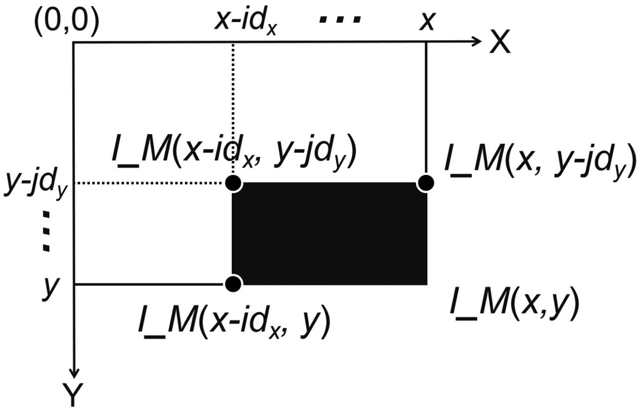
(10) f ( x − i d x < l ≤ x , y − j d y < m ≤ y ) = I − M ( x , y ) − I − M ( x , y − j d y ) − I − M ( x − i d x , y ) + I − M ( x − i d x , y − j d y ) .

Figure 2

Using integral image to calculate the summation of values within a given rectangular area.

However, it is noteworthy that values located at the upper and left boundaries of the black area in Figure 2 are excluded in the calculation of f(x, y).

2.3 MNLM

As mentioned before, the NLM is not very efficient in calculating weights and its adaptiveness is sensitive to the parameters involved. We therefore use the integral image method to speed up the weight computation process and substitute the Gaussian-weighted Euclidean distance with an unweighted one to reduce the number of control parameters. Here the MNLM is explained in more detail below.

The original image should be initially enlarged to size (n + 2D _s + 2d _s+1) × (m + 2D _s + 2d _s + 1) instead of (n + 2D _s + 2d _s) × (m + 2D _s + 2d _s) using boundary expansion algorithms (based on polynomials or cosine functions). The reason for this is that values located at the upper and left boundaries of the black area in Figure 2 are excluded during the implementation of the integral image approach, resulting in the damage of potentially useful information. The enlarged image is called N _enlarged. The general idea of using integral image for acceleration can be observed in Figure 3, which exploits the self-contained parallelization feature of NLM. Figure 3 shows that two patches named “Moving_patch” and “Static_patch” are selected when the pass through the main loop is executed. In particular, only the values in “Moving_patch” change when loops are executed. “Moving_patch” and “Static_patch” can be used to easily implement the integral image method and then to determine the unweighted Euclidean distance. Thus, the weights of the MNLM algorithm can be easily obtained and the subsequent processes can be conveniently performed. Functioning the weights calculated on a subset of “Moving_patch” and then the denoising process of the MNLM is completed.

Figure 3

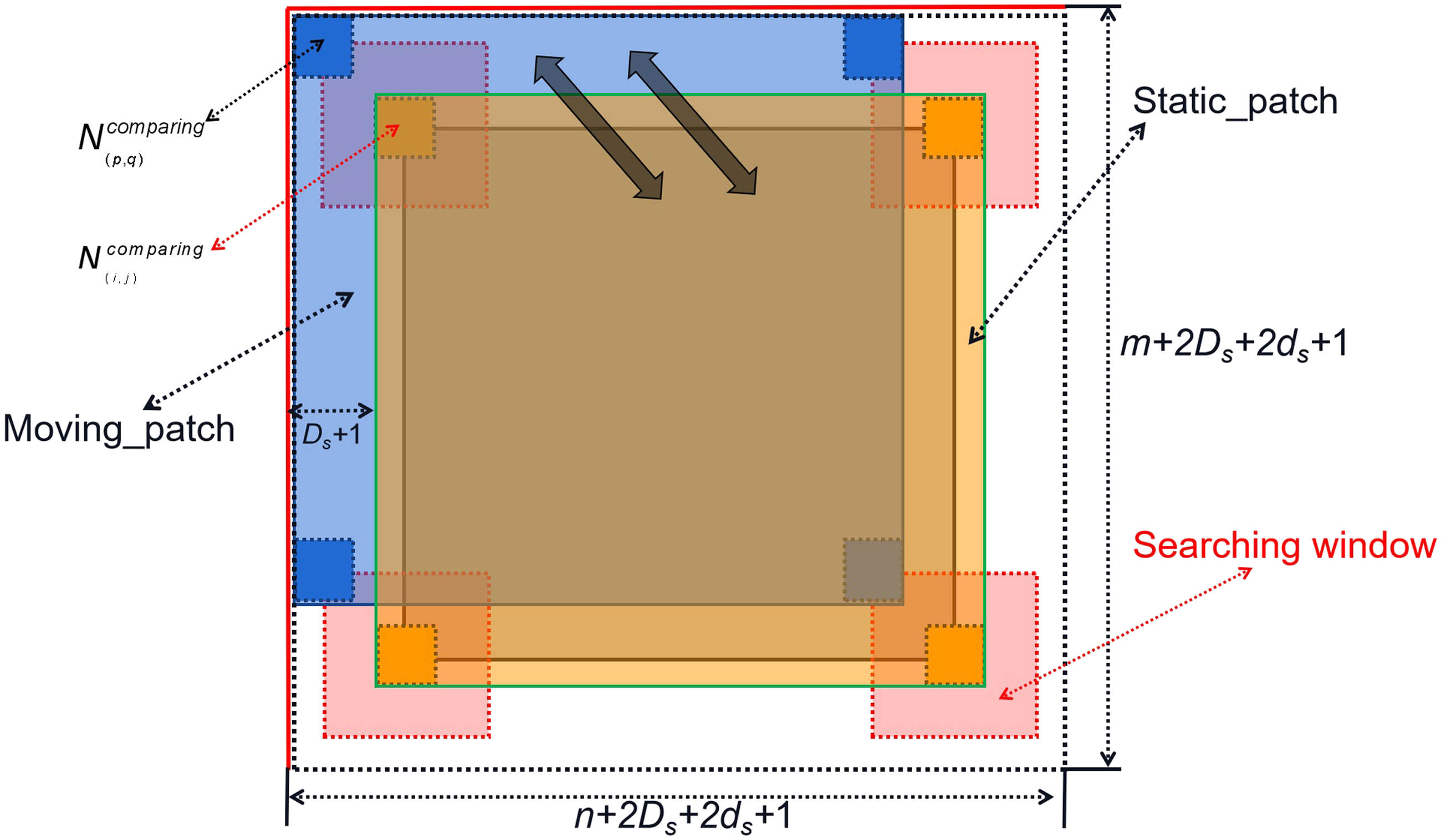
Self-contained parallelization feature of the NLM. It should be noted that the parallelization of NLM means all the data points can be considered as a whole and the weight calculation process can be simplified.

The MNLM method takes a holistic approach by simultaneously considering all the data points, which leads to a significant reduction in computational cost from O(n × m × D ²) to O(D ²) in terms of time complexity. However, this processing technique may require additional memory to store the “Moving_patch.” The modest memory loss can be easily compensated by modern hardware, making MNLM practical and effective.

Here we would like to stress two issues: (1) Skip the direct computation when (p, q) equals (i, j), and using a weight smaller than 1 for processing is vital for the quality of denoising, in order to avoid the maximum amplification of the effect of noise distortion; (2) the choice of the parameters of each filtering strategy is of great importance. However, the MNLM uses the unweighted Euclidean distance for processing, which can reduce the uncertainty and complexity of tuning the parameters involved.

2.4 Synthetic data experiments

In this section, the robustness of the modified filter is demonstrated by integrating it with the TDR [24] method. The TDR method, based on the combination of derivatives of the anomaly, is widely used to delineate the lateral boundaries of buried bodies [30] and is defined as follows:

(11) TDR = ∂ M ∂ z ∂ M ∂ x 2 + ∂ M ∂ y 2 ,

where M is the gravity anomaly, and ∂ M ∂ x , ∂ M ∂ z , and ∂ M ∂ z are derivatives along x, y, and z directions, respectively.

Here we construct a synthetic gravity model containing three prismatic bodies. The schematic structure of the synthetic gravity model with the nomenclature of buried prisms is shown in Figure 4(a). The anomaly of the gravity field is calculated on a 12 km × 12 km grid with a grid spacing of 0.1 km along the east-west and north-south directions (Figure 4(b)). The dimensions and properties of the prismatic bodies are listed in Table 1.

Figure 4

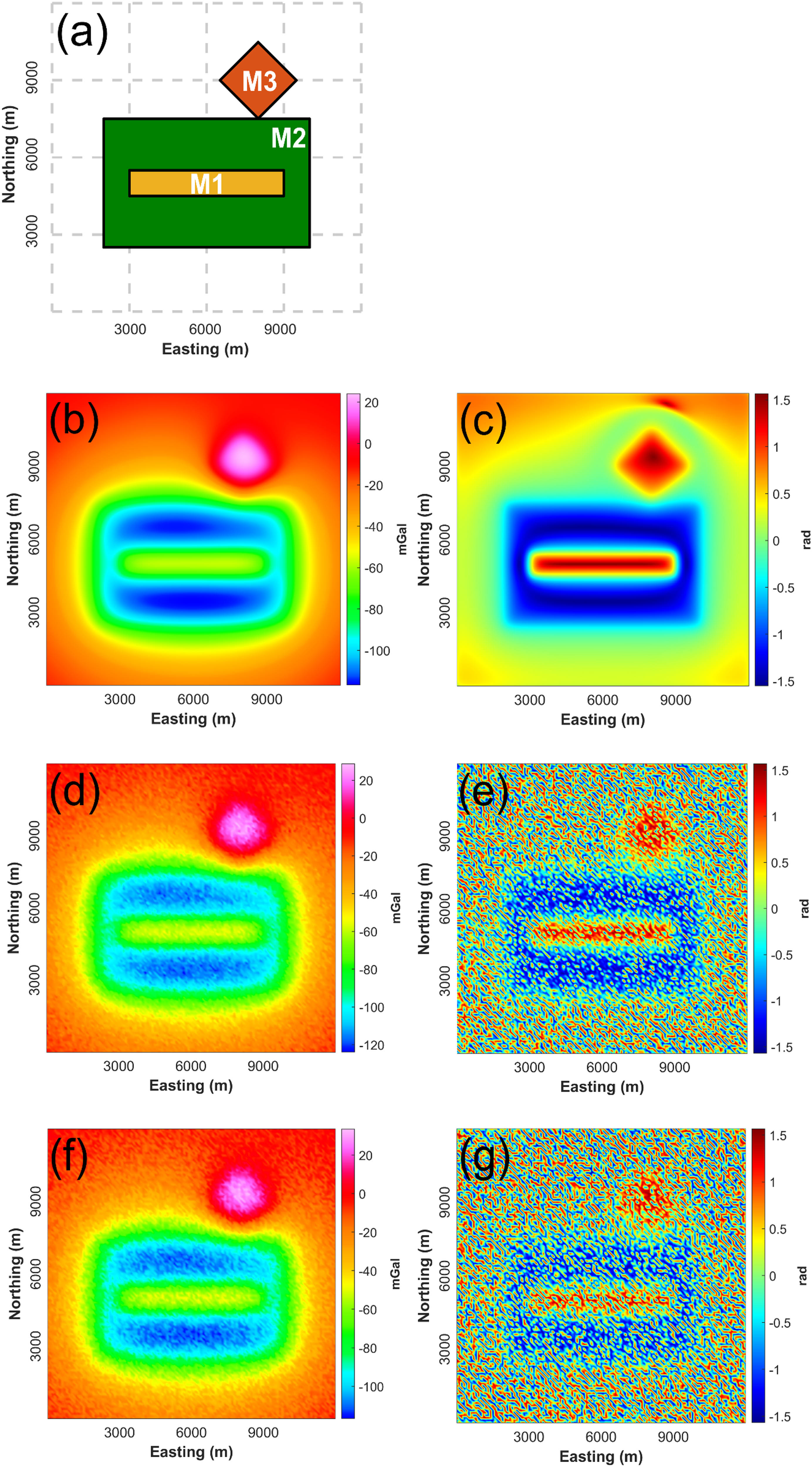
Plan view of the synthetic model. (a) buried causative prisms, (b) noise-free anomaly calculated from the synthetic model shown in (a), (c) TDR calculated from (b), (d) data contaminated with 10% random noise with uniform distribution (scenario 1), (e) TDR calculated from (d), (f) data contaminated with 10% random noise with normal distribution (scenario 2), and (g) TDR calculated from (f).

Table 1

Parameters of the synthetic model

M3	M2	M1	Parameters/model label
8,000	6,000	6,000	X-coordinates of center (m)
9,000	5,000	5,000	Y-coordinates of center (m)
1,100	6,000	6,000	Prism thickness (m)
2,100	8,000	6,000	Prism width (m)
2,100	5,000	1,000	Prism length (m)
3,000	−2,000	4,000	Density contrast (kg/m³)
300	300	200	Depth to the Top (m)
45	0	0	Strike azimuth (°)

To simulate more realistic situations, we consider two different noisy scenarios containing uniformly distributed and normally distributed noise, respectively. In scenario 1, we use random numbers from a uniform distribution with an amplitude of 11 and a noise level of 10%, and add the resulting noise component to the modeled noise-free dataset in Figure 4(b). In scenario 2, we use random numbers from a normal distribution with a noise amplitude of 17 and a noise level of 10%, and add this noise to gravity data in Figure 4(b). Figure 4(d) shows the synthetic dataset contaminated with 10% random noise with uniform distribution and Figure 4(f) shows the resulting noisy synthetic dataset corrupted by 10% random noise with normal distribution.

Figure 4(c), (e), and (g) show the TDR maps calculated from the noise-free (Figure 4(b)), noise-corrupted data with uniform distribution (Figure 4(d)), and noisy data with normal distribution (Figure 4(f)), respectively. While Figure 4(c) serves as a reference for evaluating different denoising approaches, Figure 4(e) and (g) illustrates the importance of denoising the noisy datasets before applying advanced derivative-based analyses.

2.5 Time consumption of MNLM and NLM

Before the application of the MNLM to denoise the simulated dataset, we compare the computational cost of the NLM and MNLM for processing gravity anomaly of different sizes from the quantitative perspective. All implementations are conducted on a Windows 11 operating system with 12th Gen Intel (R) Core (TM) i9-12900H CPU (2.50 GHz) and 16 GB of RAM. As shown in Figure 5, both the time consumption of NLM and MNLM increases drastically as the data size enlarges. Nevertheless, the MNLM can accelerate the calculation process approximately up to two-orders of magnitude, which verifies the effectiveness of integral image and makes the MNLM algorithm more feasible and practical to deal with real-world challenges.

Figure 5

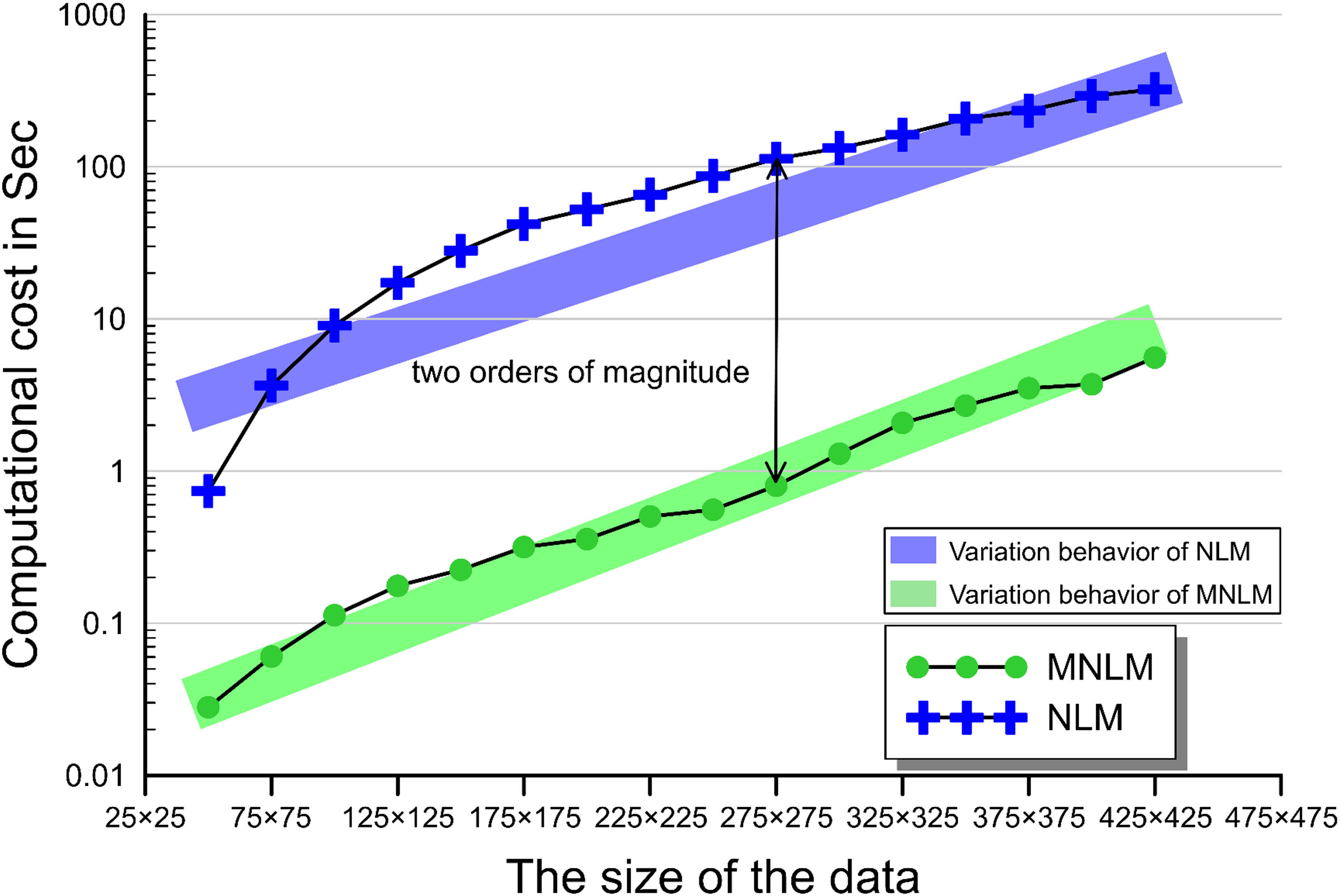
Computational cost of the MNLM and NLM for processing gravity data of different sizes. Two rectangle areas colored differently indicating the variation behavior of the two spatial-based filters show that the computational complexity increases drastically and roughly linearly as the data size enlarges.

2.6 Comparing the denoising ability of NLM and MNLM

As mentioned in Section 2.1, D _s, d _s, and h are the tuning parameters of the MNLM and NLM. Furthermore, NLM involves the extra Gaussian weight to be determined. In order to generate a relatively unbiased comparison, the weight of the Gaussian-weighted Euclidean distance of NLM is determined following the study by Manjón et al. [22], and we discuss the effect of D _s and h solely since both D _s and d _s affect the denoising process similarly (d _s is fixed to 3 in this study).

Basically, if larger values are assigned to D _s and h, denoised results will be more blurrier and degrade more structural information and vice versa. 2D topography maps of root mean square error (RMSE) values obtained by the NLM and MNLM, respectively, for different combinations of D _s and h are displayed in Figure 6. The experiment is carried out on the uniformly distributed noise-contaminated data (scenario 1). As illustrated in Figure 6, considering the added noise components obtain a small magnitude, RMSEs generally change in none-drastic manners (following the color bars) regardless of the denoising strategies (NLM and MNLM) and both D _s and h are varied linearly. Comparatively, RMSEs are more sensitive to h. Therefore, an intriguing fact is that the NLM and MNLM are not highly sensitive to D _s and h when it comes to denoise a given gravity dataset with a relatively small magnitude of corruption (Figure 6). Additionally, and most importantly, the MNLM filter yields relatively smaller RMSE values than those from the NLM, verifying the effectiveness of the modifications utilized. We thus only use MNLM to process the rest experiments instead of comparing the NLM and MNLM within each application.

Figure 6

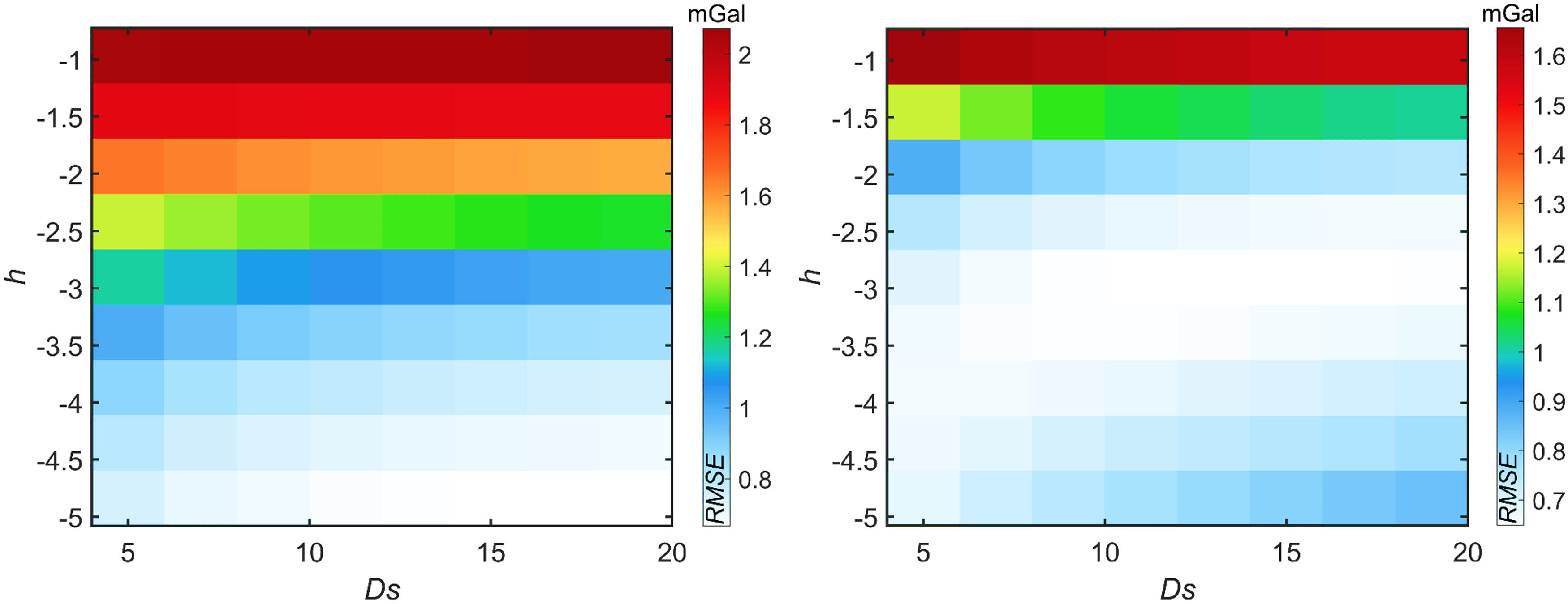
2-D topography maps of RMSE obtained using the NLM (left panel) and MNLM (right panel) for various combinations of D _s and h.

2.7 Testing MNLM with other representative methods

We apply additional three representative denoising methods, including the DCT filter [10,25,26], the SVD filter [27,28,34], and the wavelet filter [11] for comparing the quality and ability in mitigating the noise effect contaminating the synthetic gravity data. Additionally, we compare the TDR maps from all denoised images to investigate the ability of different denoising filters in determining lateral boundary maps. Notably, as mentioned above, the effectiveness of involved filters is dominated by the algorithm control parameters. Table 2 displays the tuned parameters of these filters using the same approach described in Section 2.6, namely calculating the RMSE values between the denoised results using different filters with various algorithm control parameters and the noise-free anomaly. Thus, the best control parameter can be numerically determined by the one obtaining the smallest RMSE value.

Table 2

Determined parameters of different denoising strategies for comparative studies

	Scenario 1 (uniformly distributed noise)	Scenario 2 (normally distributed noise)
MNLM	h = 0.07 × mean(∼)	h = 0.1 × mean(∼)
Wavelet	Decomposition of the image at level 3	Decomposition of the image at level 3
DCT	10 × 10	12 × 12
SVD	Threshold = 580	Threshold = 600

Notes: mean(∼) is a function calculating the average value of the input data; Ds and ds are fixed to 5 and 3, respectively, during the implementation of the NLM and MNLM; the weight of the Gaussian-weighted Euclidean distance of the NLM is determined using the approach described in ref. [22], where the normalized Gaussian weighting function has zero-mean and its standard deviation usually equals 1; we use the decomposed level 3 coefficients to reconstruct the wavelet denoised result; we preserve the upper-left 10 × 10 coefficients within the DCT domain to generate the denoised result of DCT; we discard the singular values smaller than 580 to achieve the denoising process of SVD.

Notably, the reason why we do not select the upward continuation method, the conventional noise suppression method in gravity prospecting, is that it calculates data on different horizons. However, other methods implement the noise-attenuating process on the same horizon. Moreover, the interval of continuation is manually determined, where large interval will affect the latter boundary-imaging performance (the imaged edges will not correlate with the ground truth), small interval simply cannot support satisfactory denoising performance, making the denoising process more laborious and error-prone.

Figure 7(a), (d), (g), and (j) illustrate the filtered noise components obtained using the SVD, DCT, wavelet, and MNLM methods, respectively. Figure 7(b), (e), (h), and (k) show the corresponding denoised results obtained after filtering the noise-contaminated data (Figure 4(d)) using the SVD, DCT, wavelet, and MNLM filtering methods, respectively.

Figure 7

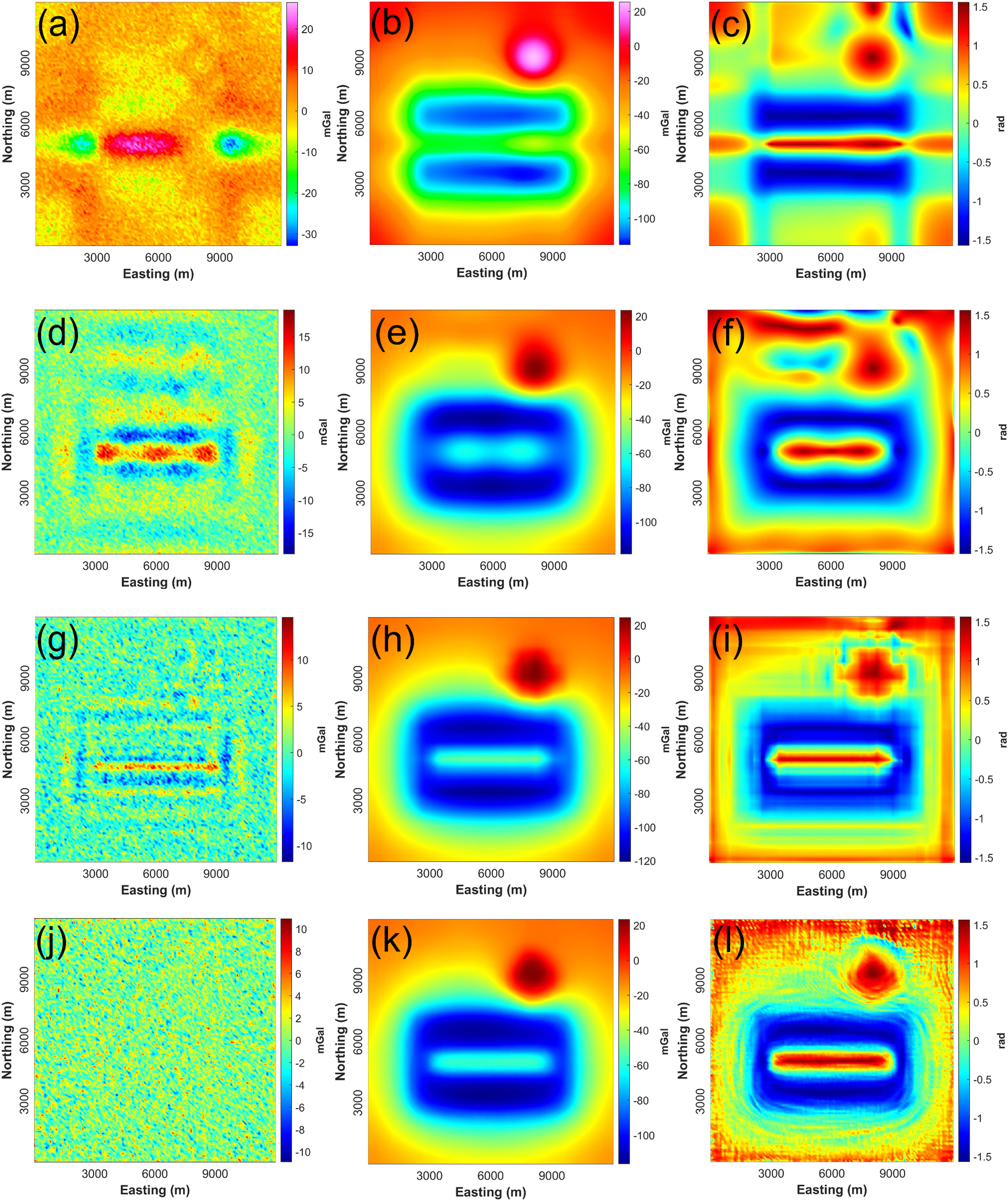
Results of applying selected denoising approaches to the noisy synthetic dataset (scenario 1). (a) Noise component obtained by the SVD, (b) filtered output using the SVD, (c) TDR calculated from (b), (d) noise component obtained by the DCT, (e) filtered result using the DCT, (f) TDR calculated from (e), (g) noise component obtained by the wavelet transform, (h) filtered data using the wavelet transform, (i) TDR calculated from (h), (j) noise component obtained by the MNLM, (k) filtered anomaly using the MNLM, and (l) TDR calculated from (k).

Comparison of the results in Figure 7(b), (e), (h), and (k), we can see that all filtering methods are capable of suppressing the high-frequency noise, dominating the noisy input data. However, when analyzing the results in more detail, we notice some significant differences between these denoising approaches. For example, we find that the output noise component via the MNLM approach barely contains structural details (Figure 7(j)), while the images resulting from the other techniques still have some low-frequency structures in the filtered noise (Figure 7(a), (d) and (g)), indicating these filters also erase some useful information. As derivative-based edge filters are sensitive to remaining noise in the input data, we use the aforementioned edge detection filter, the TDR, to further analyze the denoised images. Here we calculate the TDR of data in Figure 7(b), (e), (h), and (k). Figure 7(c), (f), (i), and (l) show the processed results of edge detection using the TDR filter. Comparing the TDR images shown in Figure 7(c), (f), (i), and (l) and also considering the reference image in Figure 4(c), we recognize that the MNLM strategy outperforms all the other approaches. After filtering the first synthetic dataset using the SVD or DCT, the remaining noise is amplified by the TDR calculation resulting in artificial structures with a false appearance in the output maps. Spurious contour and false azimuth also appear in the image based on the wavelet filtering (Figure 7(i)). However, the TDR map obtained from the data filtered by the MNLM clearly delineates the causative bodies. These observations are supported by Table 3(b) where we list the RMSE values between the TDR maps calculated from the noise-free data and the denoised data. We thus conclude that the MNLM approach provides the best denoising result and significantly improves the quality of the TDR results.

Table 3

Synthetic data: (a) RMSE values between noise-free and denoised data and (b) RMSE values between TDR maps calculated from the noise-free data and the denoised data

	RMSE	SVD filtering	DCT filtering	Wavelet filtering	MNLM filtering
Scenario 1	(a) Anomaly images	0.372	0.353	0.223	0.183
Scenario 1	(b) TDR images	0.225	0.198	0.184	0.155
Scenario 2	(a) Anomaly images	0.472	0.453	0.323	0.183
Scenario 2	(b) TDR images	0.325	0.258	0.284	0.145

Similar to the denoising process of case 1, Figure 8 yields the filtered noise components, denoised results, and further calculated TDR maps of the four methods involved, including the SVD, DCT, wavelet, and MNLM, regarding the normally distributed noise-contaminated data (scenario 2). The quality of the proposed MNLM filter yields the most satisfactory result. In the third column of Figure 8, the lateral boundaries of the sources obtain low signal-to-noise Ratio in the maps obtained by the SVD and DCT. Moreover, the azimuth of the structures and the edge of the sources in the TDR, obtained by the wavelet transform, are not of acceptable quality. In the TDR map of the denoised anomaly using the MNLM, the horizontal boundaries of the sources can be determined. It is worth stating again that the fair comparison of the selected denoising approaches regarding the second noisy case is also based on the aforementioned priori parameter tests. Tuned parameters are also presented in Table 2. Thus, the denoised images can be considered as near-optimal results for each filter. The RMSE results of this study are shown in Table 3, which show the ability of the MNLM filter to reduce noise from gravity data compared to the other three standard filters.

Figure 8

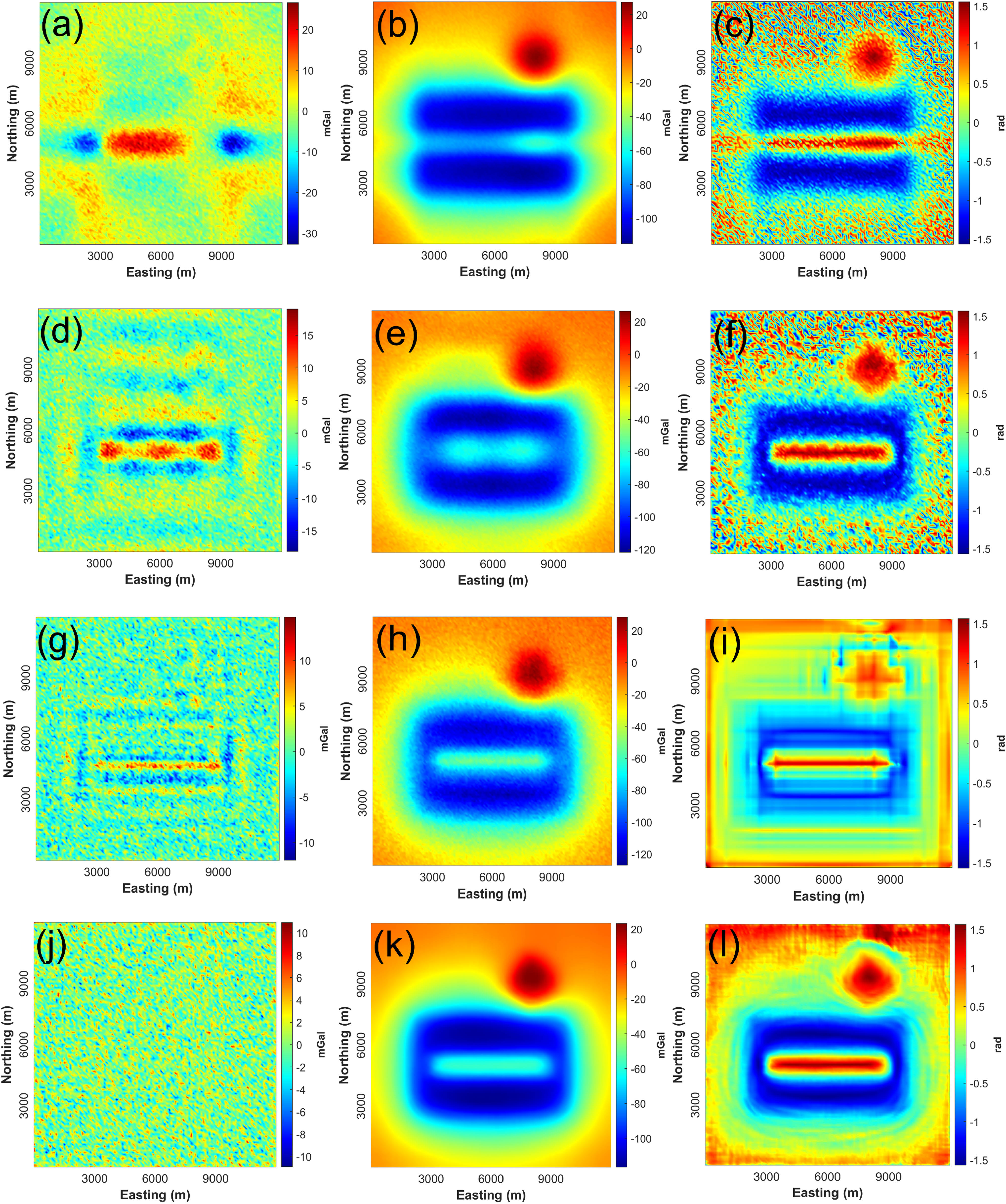
Results of applying selected denoising approaches to the noisy synthetic dataset (scenario 2). (a) Noise component obtained by the SVD, (b) filtered output using the SVD, (c) TDR calculated from (b), (d) noise component obtained by the DCT, (e) filtered result using the DCT, (f) TDR calculated from (e), (g) noise component obtained by the wavelet transform, (h) filtered data using the wavelet transform, (i) TDR calculated from (h), (j) noise component obtained by the MNLM, (k) filtered anomaly using the MNLM, and (l) TDR calculated from (k).

2.8 Application to real data

In exploration geophysics, gravity maps can be treated as useful indicators for various geological or geophysical-related applications [31,32]. When gravity field data or derivative data such as the TDR are gridded, artifacts appear along the image. In this section, we apply the MNLM filter to remove artifacts and produce good images on both gravity maps and TDR outputs. Correspondingly, the efficiency of the modified filter is compared to the aforementioned representative denoising approaches, including DCT, SVD, and wavelet transform. Ground-based gravity data from the area of Slovakia and the Mariana trench gravity anomaly obtained from WGM-2012 are utilized to achieve this study.

2.9 Ground-based gravity data

The complete Bouguer anomaly database of Slovakia (SCBA) is created from 319,915 observation points [29]. Slovakia (except for the inaccessible area) is covered by regional gravity measurements at a scale of 1:25,000, corresponding to 3–6 points/km². The gravimetric data from the Slovak database are of acceptable quality and can be used with good conscience for the interpretation of geological structures and geodetic applications [31].

Figure 9(a) shows the Bouguer gravity anomaly of the Slovak territory and Figure 9(b) gives the TDR map of Figure 9(a). The zero values of TDR are located at the boundary of the buried sources. Figure 10(a)–(d) shows the images of the filtered noise components obtained by the SVD, DCT, wavelet, and MNLM, respectively. Figure 10(e)–(h) show the denoised results derived from the filtering process of the Slovak territory data using the involved four filtering strategies. The algorithm control parameters of MNLM, wavelet, DCT, and SVD are h = 0.1 × mean (∼), decomposition of the image at level 3, preserving the upper-left 250 × 250 coefficients within the DCT domain, Threshold = 100, following the same notation in Table 2. Since there is no available ground truth in field data, the parameter tuning method presented in synthetic tests lose its worth. We thus tuned these algorithm parameters utilizing visual assessment, that is, the best algorithm parameters are selected as long as the corresponding filter gives the most satisfactory visual performance. Visual assessment can be flexibly performed on the denoised data or the further calculated derivative data. It is significant to note that visual assessment is subjective and may vary among different observers, hence its results should be interpreted with caution. Figure 11(a)–(d) displays the TDR results calculated using the denoised outputs, respectively. The TDR map computed via MNLM (Figure 11(d)) exhibits the smoothest result without damaging the noticeable structural details, especially, the edges of the anomaly sources are well enhanced with good resolution compared with the remaining results. Furthermore, the TDR results derived from other methods are corrupted by annoying artifacts (Figure 11(b)–(c)), demonstrating their deficiency in suppressing unwanted noise, while protecting potentially useful signals without producing erroneous artifacts. Clearly, the first field application validates that the newly modified filter based on non-local information can successfully remove the high frequency noise components, leading to smooth results, and minimizing the blurring effect of the gravity field derived maps. These features make the proposed filter a valuable tool for gravity data analysis.

Figure 9

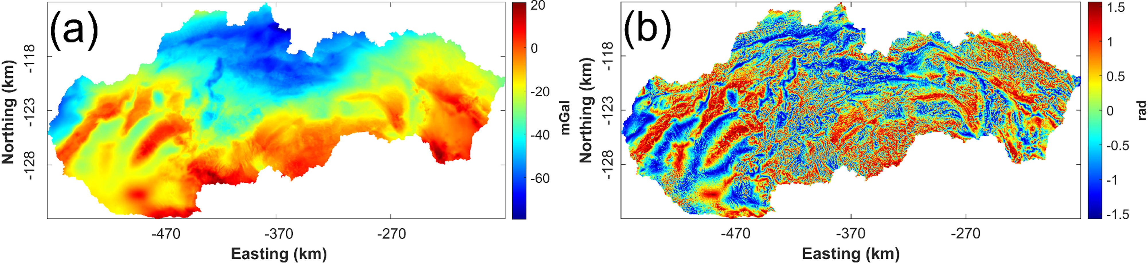
(a) Gravity anomaly of Slovakia territory and (b) TDR map calculated from (a).

Figure 10

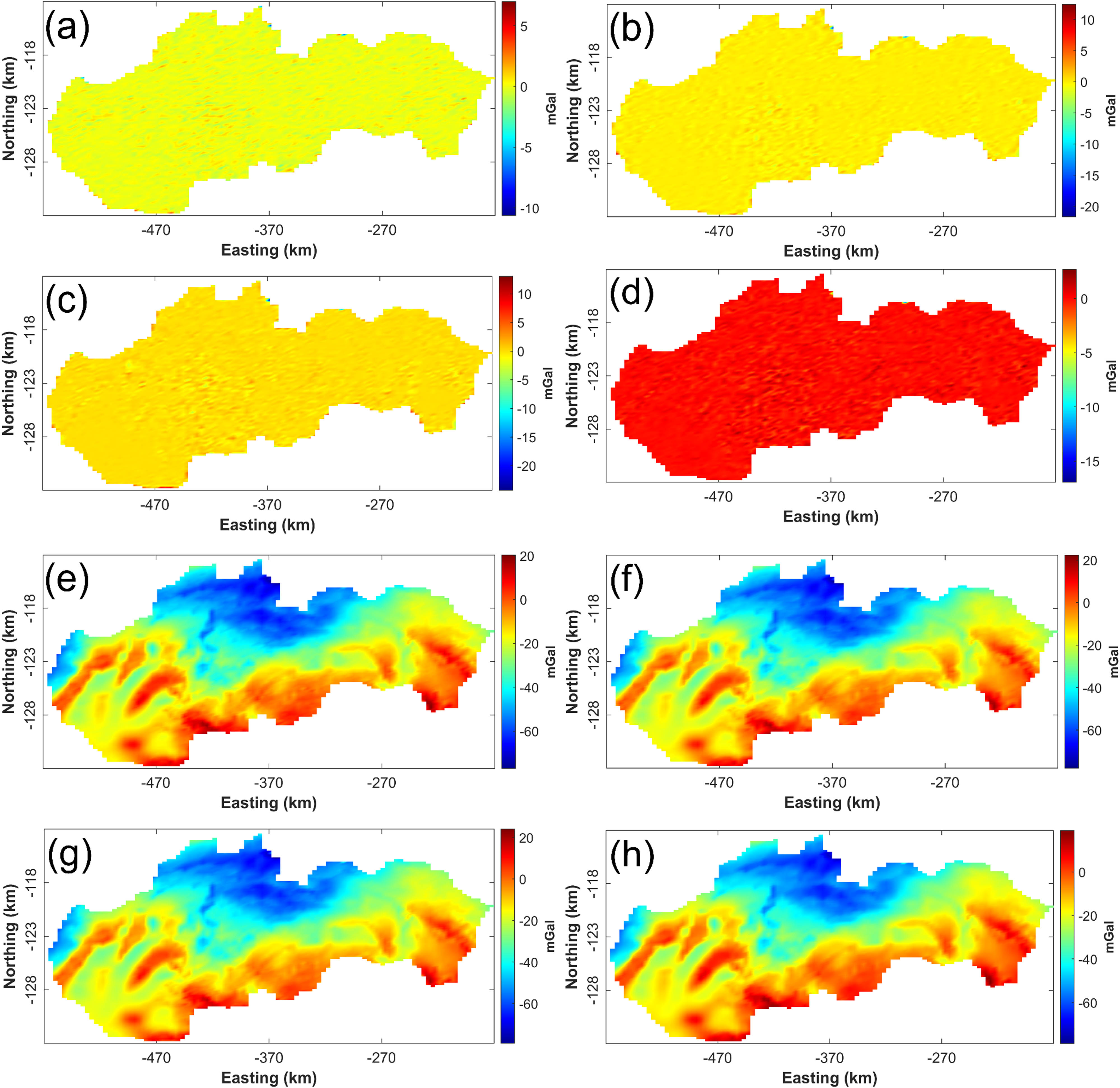
Results of applying selected denoising approaches to the Slovakia territory dataset. (a) Filtered noise using the SVD filter, (b) filtered noise using the DCT filter, (c) filtered noise using the wavelet filter, (d) filtered noise using the MNLM filter, (e) noise-attenuated result via the SVD, (f) noise-attenuated result via the DCT, (g) noise-attenuated result via the wavelet filter, and (h) noise-attenuated result via the MNLM.

Figure 11

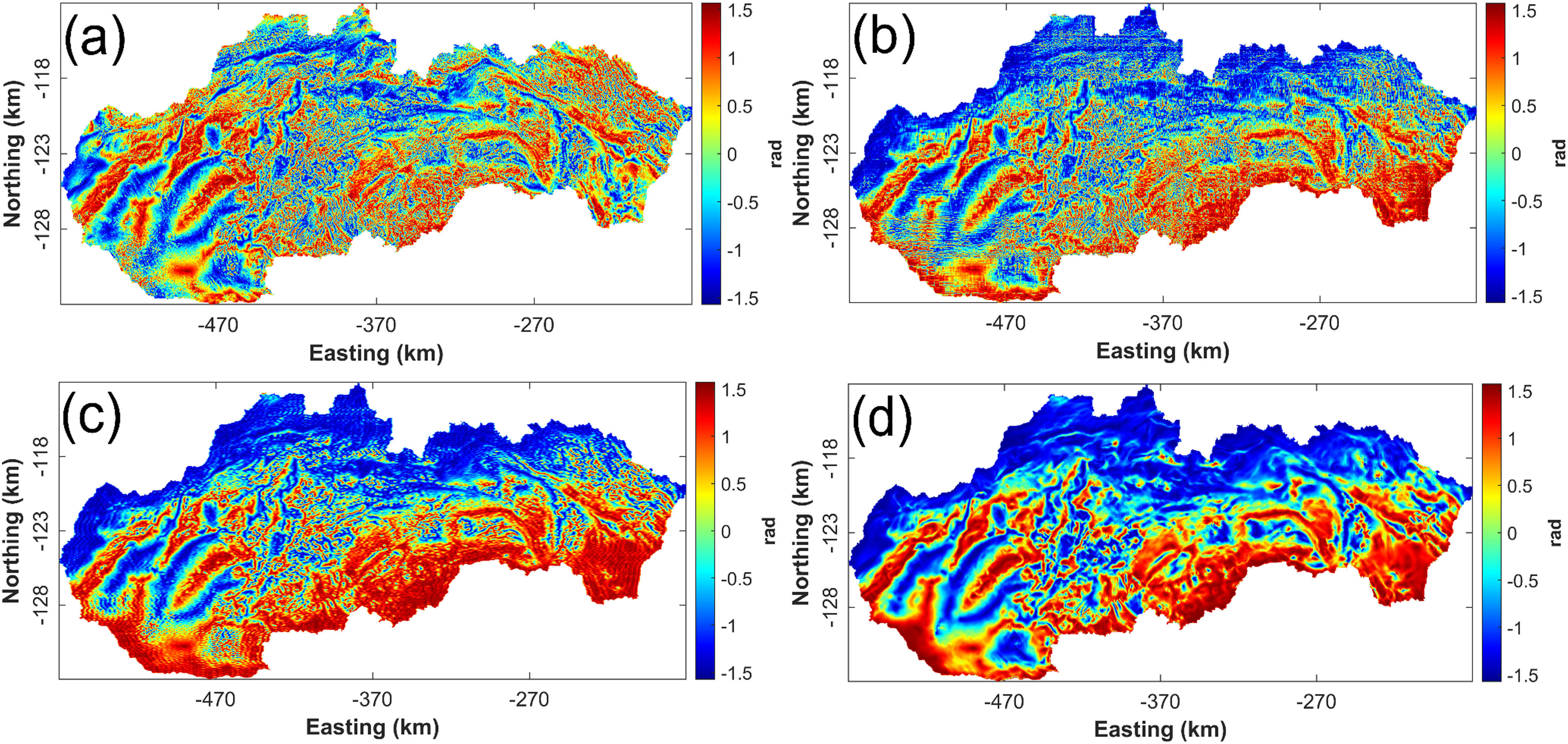
Results of applying TDR to the denoised gravity field datasets. (a) TDR map calculated from (Figure 10(e)), (b) TDR map calculated from (Figure 10(f)), (c) TDR map calculated from (Figure 10(g), and (d) TDR map calculated from (Figure 10(h)).

2.10 WGM-2012 derived gravity data

Marianna trench data (Figure 12(a)) is extracted from the WGM2012 Bouguer gravity anomaly database to investigate the quality of the filters involved further. Figure 12(b) shows the TDR result of the Mariana trench dataset. As shown in the TDR map, the coherency of the boundary or edge details is eroded by amplified noise effect due to the involved derivative calculation process, reducing the quality of the map and making the structural information impossible to be determined accurately. Therefore, in order to increase the smoothness of the edge determination map, noise removal filters should be applied. Figure 13(a)–(d) show the images of the noise components obtained by SVD, DCT, wavelet, and MNLM, respectively. The algorithm control parameter of the MNLM, wavelet, DCT, and SVD are h = 1 × mean (∼), decomposition of the image at level 3, preserving the upper-left 100 × 100 coefficients within the DCT domain, Threshold = 1,000, utilizing the same tuning process discussed in the first field data application. Figure 13(e)–(h) show the denoised results obtained after filtering the Mariana trench data using the four strategies, respectively. Subsequently, Figure 13(i)–(l) show the TDR results, computed from the denoised maps. As it can be easily observed from the TDR maps, the results generated by SVD, DCT, and wavelet are more complex than those from the MNLM method, as the massive short wave length information contained cover the general trench features. The major trench structure and other relatively small-scale curved structures are imaged with more clarity using the adapted MNLM approach. Hence, in this case, the appropriateness of the MNLM compared with SVD, DCT, and wavelet for the Mariana trench data is certified. The MNLM yields the best trending features and fewer artifacts, making the interpretation easier and more accurate. The modified filter thus can be utilized reliably for WGM-2012 gravity data, as well as in derived maps such as the TDR.

Figure 12

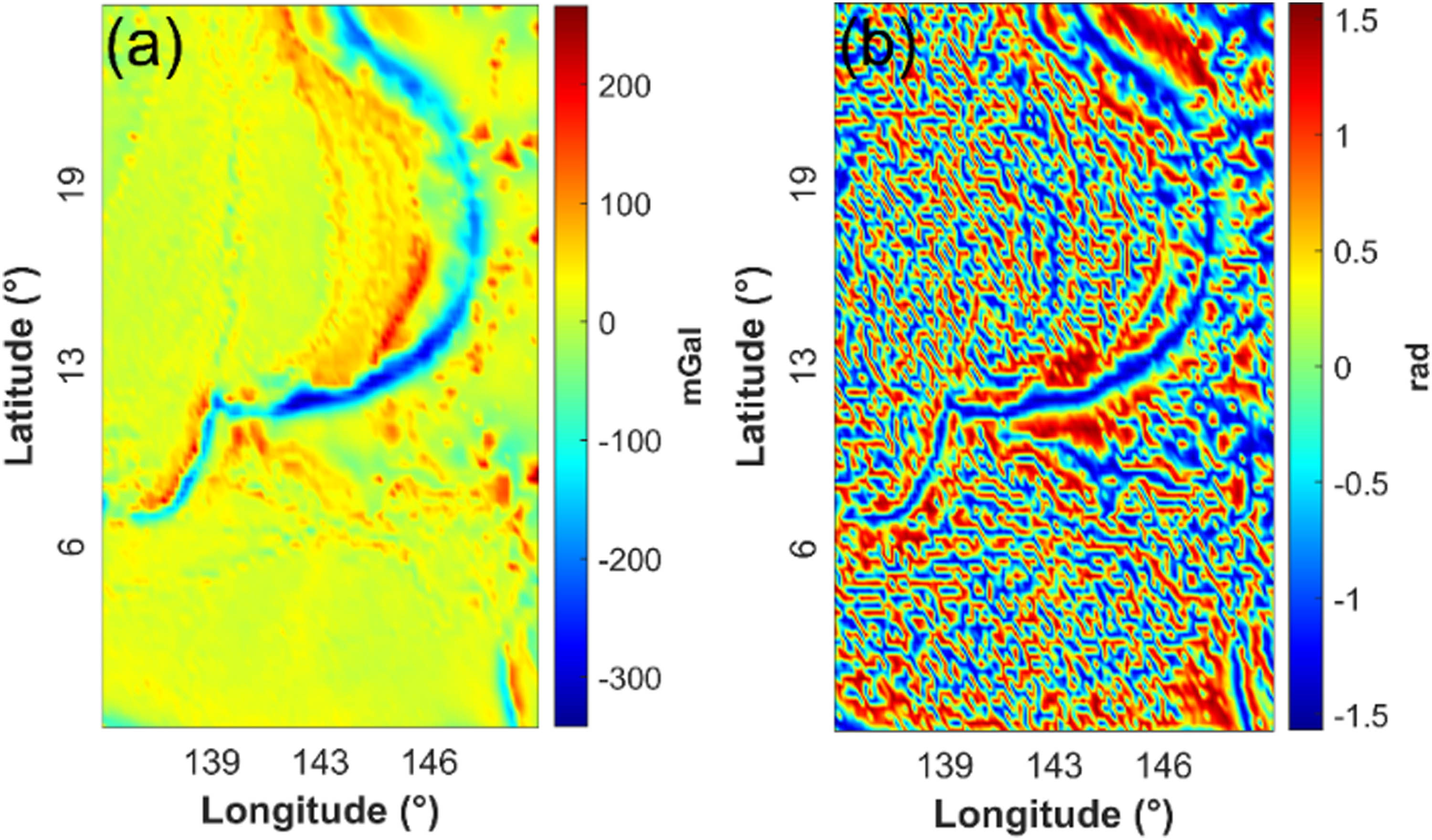
(a) The Bouguer gravity anomaly map of Mariana trench (WGM2012) and (b) TDR map calculated from (a).

Figure 13

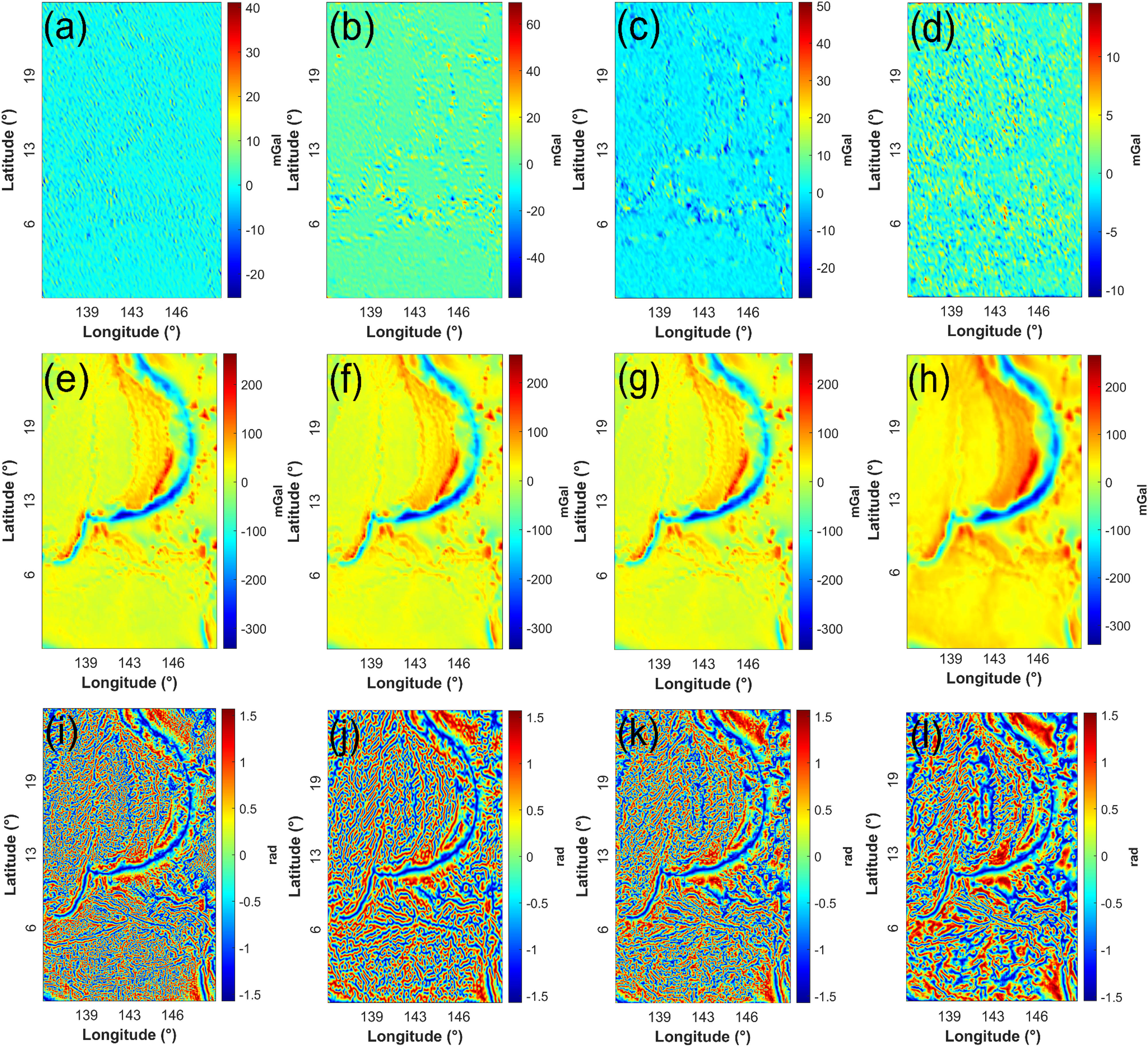
Results of applying selected denoising approaches to the Mariana trench gravity dataset. (a) Filtered noise using the SVD filter, (b) filtered noise using the DCT filter, (c) filtered noise using the wavelet filter, (d) filtered noise using the MNLM filter, (e) noise-attenuated result via SVD, (f) noise-attenuated result via DCT, (g) noise-attenuated result via wavelet, (h) noise-attenuated result via MNLM, (i) TDR map calculated from (e), (j) TDR map calculated from (f), (k) TDR map calculated from (g), and (l) TDR map calculated from (h).

3 Conclusion

Noise attenuation is a vital and basic step for gravity information processing. In order to better address this issue, we propose a MNLM filter based on unweighted Euclidean distance and integral image. The unweighted Euclidean distance is implemented to reduce the uncertainty and complexity of tuning the control parameters involved and the integral image is applied to accelerate the weight calculation process of the NLM method. Synthetic experiments and field gravity data tests from Slovak and the Mariana trench verified that MNLM can yield faster processing speed than its original form – NLM, and reduce different magnitudes of noise from different scenarios, while still finely preserve details and structures compared with other three classical and representative techniques (i.e., DCT, SVD, and wavelet filter). Furthermore, the model studies also revealed that the MNLM algorithm is not highly sensitive to its key parameters, dealing with small magnitudes of noise contamination, so that they can be relatively tuned in a more convenient manner. These features make MNLM a valuable tool for increasing the credibility of involved edge enhancement processes; therefore, source lateral boundaries can be imaged more coherently. The intrinsic reason of the high performance of MNLM lies in the weight selection process, it retains the advantage of NLM, concerning a wide range of information instead of information limited within a local neighborhood. We thus conclude that MNLM can be treated as a useful algorithm for attenuating noise situated in gravity data, helping to produce more reliable interpretations and later inversion results.

Acknowledgements

This research was supported by Researchers Supporting Project number (RSP2023R496), King Saud University, Riyadh, Saudi Arabia. This research has been done under the research project QG.23.64 of Vietnam National University, Hanoi. We would like to thank the managing editor, Dr. Jan Barabach and two capable anonymous reviewers for their suggestions that greatly improved the quality of this manuscript.

Author contributions: All authors have contributed to the conceptualization of this research and computer implementation of the methods. H.A. and A.A. worked on the mathematical theory and manuscript preparation. R.G., L.P., and S.A. carried out the data selection and discussion. D.N. and A.E. contributed to the revision process. All authors have read and agreed to the published version of the manuscript.
Conflict of interest: Authors state no conflict of interest.
Data availability statement: The Bouguer gravity anomaly of Slovakia territory is available at https://www.geology.sk/maps-and-data and the Bouguer gravity anomaly model WGM2012 is available at http://bgi.obsmip.fr/data-products/grids-and-models/wgm2012-global-model/. The computer code of MNLM is available at the GitHub platform (https://github.com/HanbingAi/Gravity-anomaly-denoising-using-Modified-Non-Local Means).

References

[1] Tronicke J, Böniger U. Steering kernel regression: An adaptive denoising tool to process GPR data. 7th International Workshop on Advanced Ground Penetrating Radar (Nantes, France). 1–4, 2013. p. 6601539. 10.1109/IWAGPR.2013.Search in Google Scholar

[2] Naprstek T, Smith R. Convolution neural networks applied to the interpretation of lineaments in aeromagnetic data. Geophysics. 2021;87(1):1–50.10.1190/geo2020-0779.1Search in Google Scholar

[3] Oruç B. Location and depth estimation of point-dipole and line of dipoles using analytic signals of the magnetic gradient tensor and magnitude of vector components. J Appl Geophysics. 2010;70:27–37.10.1016/j.jappgeo.2009.10.002Search in Google Scholar

[4] Milanfar P. A tour of modern image filtering: New insights and methods, both practical and theoretical. IEEE Signal Process Mag. 2013;30:106–28.10.1109/MSP.2011.2179329Search in Google Scholar

[5] Böniger U, Tronicke J. Integrated data analysis at an archaeological site: A case study using 3D GPR, magnetic, and high-resolution topographic data. Geophysics. 2010;75:B169–76.10.1190/1.3460432Search in Google Scholar

[6] Tomasi C, Manduchi R. Bilateral filtering for gray and color images. Proceedings of the IEEE International Conference of Computer Vision (Bombay, India); 1998. p. 836–46.Search in Google Scholar

[7] Buades A, Coll B, Morel JM. Non-local means denoising. Image Process Line. 2011;1. 10.5201/ipol.2011.bcm_nlm.Search in Google Scholar

[8] Naidu PS, Mathew MP. Analysis of geophysical potential fields: A digital signal processing approach. Amsterdam: Academic Press Inc. Elsevier Science; 1998.Search in Google Scholar

[9] Ferraccioli F, Gambetta M, Bozzo E. Micro levelling procedures applied to regional aeromagnetic data: an example from the Transantarctic Mountains (Antarctica). Geophys Prospecting. 1998;46:177–96.10.1046/j.1365-2478.1998.00080.xSearch in Google Scholar

[10] Britanak PC, Yip P, Rao K. Discrete Cosine and Sine Transforms: General Properties, Fast Algorithms and Integer Approximations. Amsterdam: Academic Press Inc. Elsevier Science; 2007.10.1016/B978-012373624-6/50007-2Search in Google Scholar

[11] Fedi M, Lenarduzzi L, Primiceri R, Quarta T. Localized denoising filtering using wavelet transform. Pure Appl Geophysics. 2000;157:1463–91. 10.1007/PL00001129.Search in Google Scholar

[12] Leblanc GE, Morris WA. Denoising of aeromagnetic data via the wavelet transform. Geophysics. 2011;66:1793–804. 10.1190/1.1487121.Search in Google Scholar

[13] Zhang DL, Huang DN, Yu P, Yuan Y. Translation-invariant wavelet denoising of full-tensor gravity–gradiometer data. Appl Geophysics. 2017;14:606–19. 10.1007/s11770-017-0649-2.Search in Google Scholar

[14] Candès E, Demanet L, Donoho D, Ying L. Fast discrete curvelet transforms. Multiscale Modeling Simul. 2006;5(3):861–99. 10.1137/05064182X.Search in Google Scholar

[15] Zeng WL, Lu XB. Region-based non-local means algorithm for noise removal. Electron Lett. 2011;47:1125–7. 10.1049/el.2011.2456.Search in Google Scholar

[16] Jain P, Tyagi V. A survey of edge-preserving image denoising methods. Inf Syst Front. 2016;18:159–70. 10.1007/s10796-014-9527-0.Search in Google Scholar

[17] Bonar D, Sacchi M. Denoising seismic data using the nonlocal means algorithm. Geophysics. 2012;77(1):A5–8. 10.1190/geo2011-0235.1.Search in Google Scholar

[18] Chan SH, Zickler T, Lu YM. Fast non-local filtering by random sampling: It works, especially for large images. IEEE International Conference on Acoustics, Speech and Signal Processing; 2013.10.1109/ICASSP.2013.6637922Search in Google Scholar

[19] Liu W, Shi Y, Ke X. Denoising seismic data using an improved nonlocal means algorithm, SEG Workshop. Reservoir Geophysics. Daqing. China: August; 2018.10.1190/REGE2018-02.1Search in Google Scholar

[20] Froment J. Parameter-Free Fast Pixel Wise Non-Local Means Denoising. Image Process Line. 2014;4:300–26. 10.5201/ipol.2014.120.Search in Google Scholar

[21] Jin W, Guo Y, Ying Y, Liu Y, Peng Q. Fast Non-Local Algorithm for Image Denoising. IEEE International Conference on Image Processing; 2007.Search in Google Scholar

[22] Manjón J, Carbonell-Caballero J, Lull JJ, García-Martí G, Martí-Bonmatí L, Robles M. MRI denoising using Non-Local Means. Med Image Anal. 2008;12:514–23.10.1016/j.media.2008.02.004Search in Google Scholar PubMed

[23] Facciolo G, Limare N, Meinhardt-Llopis E. Integral Images for Block Matching. Image Process Line. 2014;4:344–69. 10.5201/ipol.2014.57.Search in Google Scholar

[24] Miller HG, Singh V. Potential field tilt – a new concept for location of potential field sources. J Appl Geophys. 1994;32:213–7.10.1016/0926-9851(94)90022-1Search in Google Scholar

[25] Rusanovskyy D, Egiazarian KO. Video denoising algorithm in sliding 3D DCT domain. In International conference on advanced concepts for intelligent vision systems. Berlin, Heidelberg: Springer Berlin Heidelberg; 2005. p. 618–625. 10.1007/11558484_78Search in Google Scholar

[26] Pierazzo N, Morel JM, Facciolo G. Multi-scale DCT denoising. Image Process Line. 2017;7:288–308. 10.5201/ipol.2017.201.Search in Google Scholar

[27] Qiang G, Zhang C, Zhang Y, Hui L. An Efficient SVD-Based Method for Image Denoising. IEEE Trans Circuits Syst Video Technol. 2016;26:868–80. 10.1109/TCSVT.2015.2416631.Search in Google Scholar

[28] Xu Y, Cao S, Pan X. Random noise attenuation using a structure-oriented weighted singular value decomposition. Stud GeophysGeod. 2009;63:554–68. 10.1007/s11200-019-0723-8.Search in Google Scholar

[29] Zahorec P, Pašteka R, Mikuška J, Szalaiová V, Papčo J, Kušnirák D, et al. Chapter 7 – National Gravimetric Database of the Slovak Republic. Pašteka R, Mikuška J, Meurers B, editors. In: Understanding the Bouguer Anomaly: A Gravimetry Puzzle . Amsterdam: Elsevier; 2017. 113–25. 10.1016/B978-0-12-812913-5.00006-3.Search in Google Scholar

[30] Alvandi A, Ardestani VE. Edge detection of potential field anomalies using the Gompertz function as a high-resolution edge enhancement filter. Bull Geophysics Oceanography. 2023;64(3):279–300. 10.4430/bgo00420.Search in Google Scholar

[31] Alvandi A, Toktay HD, Ardestani VE. Edge detection of geological structures based on a logistic function: a case study for gravity data of the Western Carpathians. Int J Min Geo-Engineering. 2023;57(3):267–74.Search in Google Scholar

[32] Pham LT, Prasad KND. Analysis of gravity data for extracting structural features of the northern region of the Central Indian Ridge. Vietnam J Earth Sci. 2023;45(2):147–63. 10.15625/2615-9783/18206.Search in Google Scholar

[33] Shang S, Han LG, Lv QT, Tan CQ. Seismic random noise suppression using an adaptive nonlocal means algorithm. Appl Geophysics. 2013;10(1):33–40. 10.1007/s11770-013-0362-8.Search in Google Scholar

[34] Guo LF, Chen YQ, Zhao BB. Application of singular value decomposition (SVD) to the extraction of gravity anomalies associated with Ag-Pb-Zn-W polymetallic mineralization in the Bozhushan Ore Field, Southwestern China. J Earth Sci. 2021;32(2):310–7. 10.1007/s12583-020-1352-4.Search in Google Scholar

Received: 2023-07-29

Revised: 2023-09-10

Accepted: 2023-09-18

Published Online: 2023-10-16

This work is licensed under the Creative Commons Attribution 4.0 International License.

Articles in the same Issue

https://doi.org/10.1515/geo-2022-0551

Keywords for this article

gravity data; denoising; modified non-local means; Mariana trench; Slovakia

Creative Commons

BY 4.0