Semi-automated classification of layered rock slopes using digital elevation model and geological map

Hao Shang; Da-Hai Wang; Meng-Yuan Li; Yu-Hong Ma; Shi-Peng Yang; An-Bo Li

doi:10.1515/geo-2022-0526

Article Open Access

Semi-automated classification of layered rock slopes using digital elevation model and geological map

Hao Shang , Da-Hai Wang , Meng-Yuan Li , Yu-Hong Ma , Shi-Peng Yang and An-Bo Li

Published/Copyright: August 21, 2023

Published by

Become an author with De Gruyter Brill

Submit Manuscript Author Information

From the journal Open Geosciences Volume 15 Issue 1

Abstract

Layered rock slopes are the most widely distributed slopes with the simplest structure. The classification of layered rock slopes is the basis for correctly analyzing their deformation and failure mechanisms, evaluating their stability, and adopting reasonable support methods. It is also one of the essential indicators to support the evaluation of urban and rural construction suitability and the assessment of landslide hazards. However, the present-day classification methods for layered rock slopes are not sufficiently automated. In the application process of these methods, a lot of manual intervention is still needed, and sufficient strata orientation data obtained through field surveys is required, which is not effective for large-scale applications and involves high subjectivity. Thus, this study proposes a semi-automated classification method for layered rock slopes based on digital elevation model (DEM) and geological maps, which greatly reduces human intervention. On the basis of slope unit division, the method extracts structural information of slopes using DEM and geological maps and classifies slopes according to their structural characteristics. An experiment has been carried out in the northern region of Mount Lu in Jiangxi Province, and the results demonstrate the effectiveness of this semi-automated classification method. Compared to the existing manual or semi-automated classification methods, the method proposed in this article is objective and highly automated, which can meet the requirements of classification of layered rock slopes over large areas, even in the case of sparse measured orientation data.

Keywords: layered rock slope; classification; structural characteristics; DEM; geological map

1 Introduction

A slope is a discrete component of the ground surface defined principally by the angle it makes with a horizontal plane [1]. Sedimentary rocks with layered structures cover two-thirds of the land area, and many metamorphic rocks and volcanic rocks that have undergone sedimentation also have layered structural characteristics, making layered rock slopes the most widespread type of slopes in both natural and artificial slopes. In the past decades, frequent landslide disasters have caused a great number of casualties and countless property losses [2–7], which have significantly affected engineering construction activities [8–10]. Therefore, it is vital to comprehensively analyze the geological environment of construction areas, evaluate the geological suitability of engineering construction, and then carry out reasonable planning. This is closely related to people’s safety and the sustainable development of urban and rural areas. As one of the primary methods for stability analysis of rock slopes [11], the classification of layered rock slopes is the basis for correctly analyzing their deformation and failure mechanisms, evaluating their stability, and adopting reasonable support methods. It can also provide valuable references for urban and rural planning [4,12]. Consequently, the effective classification of layered rock slopes is of great research significance.

According to the application purpose, the methods for classifying layered rock slopes can be divided into the classification methods for engineering construction [13–20] and the classification methods for urban and rural planning [21,22]. The classification methods for engineering construction stem from the quantitative rock classification method proposed by Terzaghi [23], based on which the Rock Mass Rating (RMR) and Q-system were developed [24,25]. Such methods classify slopes into different stability classes based on the rock structure, considering the degree of rock weathering, joint spacing, groundwater conditions, and other factors. During the development of such methods, the RMR and Q system were commonly used as starting points for developing other specialized classification methods. Among the methods based on RMR, Ming Rock Mass Rating (MRMR) and Slope Mass Rating (SMR) are the most widely used [14,26,27,28]. MRMR classifies slopes into five adjustment levels and is mainly used for the classification of slopes in mining areas [29–31], while SMR classifies slopes into five stability levels and is primarily used for the classification of slopes in civil engineering [32–37]. Among the methods based on Q-system, the Q-slope [19] proposed in recent years is the most representative. Q-slope is mainly used to classify rock slopes excavated on-site into three categories [27,38,39]: stable slopes, unstable slopes, and slopes with uncertain stability. Based on the classification results, potential adjustments to the dip angles of slopes are made when necessary during the construction period. In recent years, neural networks and deep learning techniques have been frequently used in such approaches and have yielded promising results [40–42]. The classification methods for engineering construction emphasizes the integrity of the rock mass and focuses on analyzing the engineering properties of the slope rock mass. However, the application of this type of methods is limited to specific major projects because of the need for detailed measurement data of rock mass.

The classification methods for urban and rural planning originate from the slope classification criteria proposed by Jin [43], which is summarized according to the practices of hydropower engineering. Such methods classify slopes mainly according to the geometric relationship between the slope surface and the strata surface [44]. Considering that geological structure and the shape of slope has an important influence on slope stability [45–48], these methods focus on analyzing the impact of overall slope structure on slope deformation and stability. Classification based on this idea was achieved mainly by manual means in the early stage, which is time-consuming, irreproducible, and can be easily influenced by subjective factors [21]. In recent years, a few researchers have started the study of automatic classification of layered rock slopes. Particularly noteworthy is the framework for sensitivity analysis of layered rock slopes proposed by Lin et al. [22]. Using this framework, semi-automated slope classification is achieved with the help of ArcGIS and eCognition software. Following the idea of such methods, the orientation of strata can be calculated based on geological maps and digital elevation model (DEM) data without the need for measurement data of rock mass, which well meets the requirements of layered rock slope classification over large areas in urban and rural planning. However, the current methods still require a lot of manual intervention and are not yet automated enough for large-scale applications.

To facilitate the large-scale classification of layered rock slopes in urban and rural planning, this study proposes a semi-automated classification method for layered rock slopes based on DEM data and geological maps. Specifically, this method extracts slope units based on DEM data. Thereafter, according to the classification scheme of layered rock slopes, the structural parameters of slopes are calculated based on geological maps and DEM data to classify layered rock slopes over large areas. The remainder of this article is organized as follows: Section 2 describes the study area and input data, Section 3 presents the methodology, Section 4 presents the experimental results, Section 5 presents the discussion, and Section 6 presents the conclusion and future work.

2 Study area and input data

2.1 Study area

Mount Lu, located in Jiangxi Province, China, covers an area of 300 km² with a length of about 25 km and a width of about 10 km. It is oval in shape and stretches in the northeast-southwest direction. This area generally contains two tectonic regions: the northern region is controlled by fold structures, and the southern region is controlled by fault structures [49].

The study area is located in the northern region of Mount Lu, with a geographical range between 115 ° 54 ′ – 116 ° 3 ′ E and 29 ° 30 ′ – 29 ° 39 ′ N (Figure 1a). The land predominantly consists of hills and the slopes are mainly naturally formed layered rock slopes distributed with sparse measured strata orientation data (Figure 1c). The local strata are basically not covered by volcanic rocks and loose layers, and the structure is relatively complete. The exposed strata include the strata of Sinian (Z), Cambrian (€), Ordovician (O), and Silurian (S), together with the outcrops of Cretaceous (K) intrusive rocks and the sediments of Quaternary (Q). In the southern region of the study area, the Donggu syncline, Dayueshan anticline, and Wulaofeng monocline are developed from northwest to southeast. Besides, secondary valleys are developed in some areas.

Figure 1

Study area in the northern region of Mount Lu in Jiangxi Province, China. (a) Location of the study area, observed from remote sensing images of Google Earth platform. (b) The 1:50,000 geological map of the study area proposed by Jiangxi Geological and Mineral Exploration and Development Bureau. (c) The digital geological map of the study area. (d) 5-meter resolution DEM of the study area.

2.2 Input data

DEM with 5-meter spatial resolution (Figure 1d), vector stratum and orientation point data of digital geological map (Figure 1c) are used for classifying layered rock slopes in this study. The digital geological map is derived from the 1:50,000 geological map (Figure 1b) proposed by Jiangxi Geological and Mineral Exploration and Development Bureau. There are 29 measured orientation points in the study area on the geological map.

3 Methodology

Based on the determination of the classification scheme of layered rock slopes according to their structural characteristics, this study proposes a semi-automated classification method for layered rock slopes. The method mainly involves the following steps (Figure 2): (1) extracting hill boundaries based on DEM data, (2) dividing the hill boundaries into slope units using ridge lines, (3) calculating the structural parameters of each slope based on the calculation results of the strike and dip direction of slope as well as strata orientation, and (4) classifying slopes based on their structural parameters according to the classification scheme of layered rock slopes. All steps are automatically implemented except for step (1), where the ArcGIS platform is utilized.

Figure 2

Flow diagram of the layered rock slope classification method.

3.1 Designing the classification scheme of layered rock slopes

The structural parameters that have the greatest impact on the stability of layered rock slopes are dip angle of strata constituting the slope, angle between dip direction of slope surface and that of strata, and angle between strike of slope surface and that of strata. The geometric relationship between strike of slope surface and that of strata can be divided into three types [50]: perpendicular, oblique, and parallel. And layered rock slopes can be classified into three types accordingly: perpendicular slopes, oblique slopes, and near horizontal slopes. Furthermore, according to the geometric relationship between dip direction of slope and that of strata, near horizontal slopes can be subdivided into three categories [51]: horizontal slopes, dip slopes, and anti-dip slopes.

In summary, based on structural characteristics, layered rock slopes can be classified into five categories (Table 1): perpendicular slopes, oblique slopes, horizontal slopes, dip slopes, and anti-dip slopes. A detailed classification scheme of layered rock slopes is proposed, as shown in Table 2.

Table 1

Geological models of different types of layered rock slopes [52]

Slope type	2D Geological model	3D Geological model	Description
Horizontal slope			The slope surface and strata have approximately equal strikes. And the dip angle of strata is close to 0.
Dip slope			The slope surface and strata have approximately equal strikes and dip directions.
Anti-dip slope			The slope surface and strata have approximately equal strikes and roughly opposite dip directions.
Oblique slope			The strike of the slope surface is obliquely intersected with that of strata.
Perpendicular slope			The strike of the slope surface is perpendicularly intersected with that of strata.

The translucent green sheets in the 3D geological models represent slope surfaces.

Table 2

Classification scheme of layered rock slopes [50,51]

Slope type	Characteristics
Horizontal slope	β < 10 °	α ≤ 5 °
Dip slope		θ < 10 °
Anti-dip slope		θ > 170 °
Oblique slope	10 ° ≤ β ≤ 60 °
Perpendicular slope	60 ° < β < 90 °

α represents the dip angle of strata, β represents the angle between the strike of slope surface and that of strata, and θ represents the angle between the dip direction of slope surface and that of strata.

3.2 Extracting hill boundaries with the constraints of terrain feature lines

To effectively classify slopes, the boundary of each slope needs to be obtained first. At the same time, the acquisition of hill boundaries can serve as a prerequisite for the generation of slope boundaries. As important landform elements, hill boundaries can be generated by extracting basin boundaries through hydrological analysis of reverse DEM [53] and then performing raster-to-vector conversion [54–56]. However, the terrain in mountainous regions is complex and has a multi-scale issue, leading to a problem that the hill boundaries extracted by this method are very fragmented, which cannot meet the needs of geographic research and require further manual processing. Therefore, some optimizations are made on the basis of the above method by correlating the broken hill boundaries using terrain feature lines, through which hill boundaries on the macro-geographic scale can be generated.

The flow diagram of the hill boundary extraction process is shown in Figure 3. First, the ridge lines, valley lines, and broken hill boundaries are extracted using ArcGIS platform. The ridge lines and valley lines need to be filtered and correlated with human intervention to improve their quality. And the tiny polygons in the broken hill boundary layer need to be eliminated. Then, the broken hill boundaries are correlated automatically using terrain feature lines to generate hill boundaries on the macro-geographic scale. This section focuses on correlating separated polygons using ridge lines, valley lines, and without constraints.

Figure 3

Flow diagram of hill boundary extraction.

3.2.1 Correlating separated polygons using ridge lines

The number of ridge lines determines the number of hill boundaries eventually obtained. And each hill boundary will definitely contain its corresponding ridge line. Accordingly, the polygons with the same ridge line passed by can be merged to generate a preliminary hill boundary.

The specific steps of correlating separated polygons with the same ridge line passed by are as follows:

Obtaining polygons in the vector layer of hill boundaries and ridge lines, respectively. Read the vector data of hill boundaries and ridge lines, respectively, to get the set of polygons MB = { M m | m = 1 , 2 , … , MN } ( MN is the number of polygons) and the set of ridge lines RL = { R r | r = 1 , 2 , … , RN } ( RN is the number of ridge lines).
Adding an Id attribute to each polygon in MB and assigning values. Add an attribute Id for each polygon. The attribute Id uniquely marks a ridge line and is initialized to −1. For each polygon, traverse the set of ridge lines RL, if any point on R r is within the polygon, then set the value of its Id to r.
Correlating separated polygons in MB. Read the Id attribute of each polygon. Merge polygons with the same Id to get the set of preliminarily generated hill boundaries AP = { A a | a = 1 , 2 , … , AN } ( AN is the number of preliminarily generated hill boundaries, which equals the number of ridge lines) and the set of uncorrelated polygons UP = { U u | u = 1 , 2 , … , UN } ( UN is the number of uncorrelated polygons), respectively.

3.2.2 Correlating separated polygons using valley lines

For each polygon representing a preliminarily generated hill boundary in AP, select its adjacent polygons and use the valley lines as a constraint to correlate polygons satisfying specific rules (Table 3). The correlation method is described below:

Table 3

Correlating rules with the valley lines as constraints

Rules	Natural language	Formal language
Rule 1	If no valley line passes through the uncorrelated polygon U u , which is adjacent to more than one polygon in AP and has the longest common boundary with A a , then merge U u and A a .	If Fid == −1
		And count > 1
		And A a ′ == A a
		Then, union ( A a , U u )
Rule 2	If no valley line passes through the uncorrelated polygon U u , which is only adjacent to A a in AP, then merge U u and A a .	If Fid == −1
		And count == 1
		Then, union ( A a , U u )
Rule 3	If a valley line passes through the uncorrelated polygon U u , which is adjacent to more than one polygon in AP and has the longest common boundary with A a , and A a and U u lie on the same side of the directed line segment, then merge U u and A a .	If Fid ! = −1
		And count > 1
		And A a ′ == A a
		And Dir ′ == Dir
		Then, union ( A a , U u )
Rule 4	If a valley line passes through the uncorrelated polygon U u , which is only adjacent to A a in AP, and the length of the common boundary between U u and A a is not less than half of the perimeter of U u , and A a and U u lie on the same side of the directed line segment, then merge U u and A a .	If Fid ! = −1
		And count == 1
		And scale > = 0.5
		And Dir ′ == Dir
		Then, union ( A a , U u )

First, add attributes to each polygon in UP and assign values following the steps below:

For a polygon U u in UP, add the attributes Fid, Line, and Dir to it. Among them, Fid uniquely marks a valley line and is initialized to −1; Line represents a directed line segment used to determine the spatial relationship between U u and the valley line; Dir indicates that U u is on the left or right side of Line and takes the value of “left” or “right.”
Generating directed line segments. Read the valley line data to get the set of valley lines VL = { V v | v = 1 , 2 , … , VN } ( VN is the number of valley lines). For the points on each valley line V v , take two adjacent points in sequence to generate a directed line segment. Count the number of directed line segments intersecting the polygon U u among the obtained directed line segments. If the number is 1, the Fid of U u is set to v, and the Line attribute of U u is set to the directed line segment; if the number is greater than 1, the Fid of U u is set to v, and the Line attribute of U u is set to the directed line segment consisting of the first point of the first directed line segment and the end point of the last directed line segment.
Calculating the value of the attribute Dir. Use each point on the boundary of polygon U u to generate a pair of vectors with the first and last points of the corresponding directed line segment Line, respectively, and calculate the cross product of the two vectors using equation (1). If the proportion of cross products greater than 0 is not less than 50%, set the Dir attribute of U u to “left”; otherwise, set the value of Dir to “right.”

(1) ( P 1 − P 3 ) × ( P 2 − P 3 ) = ( x 1 − x 3 ) ( y 2 − y 3 ) − ( y 1 − y 3 ) ( x 2 − x 3 ) ,

where P 3 is a vector represented by the coordinates of a point on the boundary of polygon U u , P 1 and P 2 are two vectors represented by the coordinates of the first and last points of the directed line segment Line, and x i and y i denote the x and y coordinates of P i .

Next recursively process the polygons in the UP as follows:

For each polygon A a in the set AP, traverse UP, and if there exists a polygon U u adjacent to A a , compute the constraint parameters. First, Read the attribute value Fid of U u and set it to the value of the parameter Fid. Second, count the total number of polygons in AP adjacent to U u and set this total to the value of the parameter count. Third, find the polygon A a ′ in AP adjacent to U u , which has the longest common boundary with U u . Next read the Dir attribute of U u and use the Line attribute of U u to calculate the Dir’ attribute of A a . At last, calculate the ratio of the length of the common boundary between U u and Aa to the perimeter of U u and set it to the value of the parameter scale.
Determine whether the constraint parameters obtained in the previous step satisfy the constraints in Table 3. Remove U u from UP if any of the constraints are satisfied. Meanwhile, add U u to the set TP.
After traversing UP, merge all the polygons in TP and A a to generate a new polygon and replace A a with the new polygon.
Loop through steps (1)–(3) until all the polygons in the set AP are traversed, and then continue with the next recursion.

3.2.3 Correlating separated polygons without constraints

After the above two correlation operations, there are polygons still remaining separated. These polygons can be treated by borrowing the idea of correlating polygons using valley lines. Without the valley lines as a constraint, it is not necessary to consider the attributes of uncorrelated polygons, so each separated polygon can be merged into a polygon in AP which has the longest common boundary with it. Recursively process uncorrelated polygons until there are no separated polygons. At this step, the extraction of hill boundaries is completed.

3.3 Generating slope units

As important geomorphic entities, slope units are well suited for landslide susceptibility modeling and zonation, as well as for hydrological and geomorphological studies [57]. The slope unit can be considered as a part of the slope or as half of the catchment basin [58]. Thus, the results obtained by dividing the hill boundaries using ridge lines are taken as the slope units.

Each hill boundary can be divided into two slope units using the corresponding ridge line as the dividing line. However, some ridge lines may not intersect with any hill boundary and needs to be further processed to meet the requirements of slope unit delineation.

The specific steps of slope unit generation are as follows:

Calculating the strike of each ridge line. First, read the points contained by a ridge line. From the starting point, take two adjacent points in order to generate a directed line segment, and calculate the azimuth of the directed line segment. Next sort all the azimuths in reverse order by value and calculate the difference between two adjacent azimuths in sequence. Group the azimuths by dividing the azimuths with a difference less than the parameter T into the same group. Calculate the mean value of the group with the largest number of azimuths, and the result is the strike of the ridge line (all strikes and dip directions in this work are represented in the form of azimuth). The strike of each ridge line can be calculated following the above steps.
Extending and trimming ridge lines. The topological relationship between ridge lines and hill boundaries can be summarized into four cases (Figure 4). The idea of extending and trimming a ridge line is: Determine the topological relationship between the starting point of the ridge line and the hill boundary, and if they intersect, find the intersection point and remove the points outside the hill boundary; otherwise, extend the ridge line by adding a new point and calculate the coordinates of the new point according to equation (2), and continue this process until the ridge line intersects with the hill boundary. The end point of the ridge line is treated similarly to the starting point.
(2) x ′ = P x + Dis * cos ⁡ ( strike ) y ′ = P y + Dis * sin ⁡ ( strike ) ,
where x ′ and y ′ are the x and y coordinates of the new point, P x and P y denote the x and y coordinates of the start or end point of the ridge line, Dis is the average distance between two adjacent points in the first three points of the ridge line, and strike is the strike of the ridge line represented in the form of azimuth.
Dividing the hill boundaries to generate slope units. Divide the points contained in a hill boundary into two point sets using the directed line segment consisting of the first and last points of the corresponding ridge line. Then, add the points contained in the ridgeline to the two point sets. Two slope units can then be generated, i.e., the left and right slopes.

Figure 4

Four situations that may be encountered when extending and trimming a ridge line and the corresponding treatments. (a) The start and end points of the ridge line are both located within the hill boundary, in which case the ridge line should extend at both ends. (b) The start and end points of the ridge line are both located outside the hill boundary, in which case the ridge line should be trimmed at both ends. (c) The start point of the ridge line is located within the hill boundary, and the end point is located outside the hill boundary, in which case the ridge line should extend at the start point and be trimmed at the end point. (d) The start point of the ridge line is located outside the hill boundary, and the end point is located within the hill boundary, in which case the ridge line should be trimmed at the start point and extend at the end point. (e) The result of extending and trimming a ridge line.

3.4 Calculating the structural parameters of slopes

The structural characteristics of layered rock slopes are the most critical factors affecting their stability, mainly including dip angle of strata, the angle between the strike of slope surface and that of strata, the angle between the dip direction of slope surface and that of strata, etc. Therefore, the prerequisite for classifying layered rock slopes is to obtain the strike and dip direction of slope surface and the orientation of strata.

3.4.1 Calculating the strike and dip direction of slope surface

Since this work uses ridge lines to divide the hill boundaries to generate slope units, the strike of the ridge line is used as the strikes of both the left slope and the right slope, i.e., ρ lSlope = ρ rSlope = strike ( ρ lSlope represents the strike of the left slope, ρ rSlope represents the strike of the right slope, and strike is the strike of the ridge line). The dip direction of slope surface can be calculated using equation (3).

(3) θ lSlope = strike + 90 , strike < 270 strike − 270 , strike ≥ 270 θ rSlope = strike + 270 , strike < 90 strike − 90 , strike ≥ 90 ,

where θ lSlope denotes the dip direction of the left slope, θ rSlope represents the dip direction of the right slope, and strike is the strike of the ridge line.

3.4.2 Calculating the orientation of strata

In ideal conditions, the measured orientations on the geological maps can meet the needs of strata orientation calculation. An orientation point can be generated for each orientation on the geological maps, and a point set containing orientation information can then be formed. And when the measured orientation data on the geological maps are insufficient, the three-point or four-point method can be used to calculate the orientation of strata adaptively using DEM data and digitized geological maps [59]. Specifically, when the application conditions of the four-point method and the three-point method are both met, the four-point method is preferred for calculating the orientation as its calculation results have a smaller error. Then, a point set containing measured and calculated orientation data can be obtained.

For each slope, all points located within it are filtered from the point set. Count the dip direction information contained in each point by interval, and find the interval with the largest number of values. Thereafter, find the points corresponding to these values and use them as the dominant point set of the current slope. Calculate the mean value of the dip direction and dip angle of all points in the dominant point set as the dip direction and dip angle of strata in the current slope, respectively.

The strike of strata can be calculated using equation (4).

(4) ρ strata = ( θ strata + 90 ) MOD 180 ,

where ρ strata represents the strike of strata, θ strata denotes the dip direction of strata, and MOD is the remainder operator.

3.4.3 Calculating the structural parameters of slopes

Calculate the structural parameters of slope based on the strike and dip direction of slope surface and the orientation of strata calculated using the method proposed in Sections 3.4.1 and 3.4.2. The angle between dip direction of slope surface and that of strata can be obtained simply by calculating the difference between these two values. And the dip angle of strata can be derived using the method proposed in Section 3.4.2.

Here the calculation of the angle between the strike of slope surface and that of strata needs to be elaborated. In this study, for the convenience of calculation, the strikes of slope surface and strata are expressed by a single azimuth. But the fact is that a strike implies two directions, and their values differ by 180 degrees. Therefore, the angle between strike of slope surface and that of strata can be determined using equation (5).

(5) β = | ρ slope − ρ strata | , | ρ slope − ρ strata | < = 90 180 − | ρ slope − ρ strata | , 90 < | ρ slope − ρ strata | < = 180 | ρ slope − ρ strata | − 180 , 180 < | ρ slope − ρ strata | < = 270 360 − | ρ slope − ρ strata | , 270 < | ρ slope − ρ strata | < 360 ,

where β represents the angle between the strike of slope surface and that of strata, ρ slope represents the strike of slope surface, and ρ strata represents the strike of strata.

3.5 Classifying slopes and calculating related attributes

This section aims at classifying slopes and calculating some crucial attributes. The calculation of strike and dip direction of slope surface, as well as orientation of strata in the slope, is described in detail in Section 3.4. The plan-view area of a slope can be obtained by calculating the area of the corresponding vector polygon. In addition to the classification of layered rock slopes, this section details the calculation of dip angle and surface area of slope and the division of shady and sunny slopes.

First, the structural parameters of a slope imply its structural characteristics. Thus, layered rock slopes are classified according to their structural parameters. The rules for classifying layered rock slopes based on the values of the three structural parameters are shown in Table 2.

Second, the dip angle of a slope is obtained by averaging the dip angles of a series of slope profiles. For each slope, collect a series of profiles by taking a profile every 100 m along its strike. The dip angle of a slope profile can be derived from the ratio of slope length and height. The calculation method is shown in equation (6). Finally, the average value of the dip angles of all slope profiles is taken as the dip angle of this slope.

(6) dip angle = arctan slopeHeight slopeLength ,

where dip angle denotes the dip angle of the slope, slopeHeigh t represents the height of the slope, and s lopeLength is the length of the slope.

Third, the calculation of the surface area of slopes is based on DEM data. To obtain the surface area of a slope, the centroids of DEM pixels covered by the slope are connected to generate a 3D triangular network, and then the areas of all the triangles in the triangular network are summed up.

Finally, according to the dip direction of slope, the slopes are divided into shady and sunny slopes, and the division rules are shown in Table 4. This attribute implies the light exposure characteristics of slopes and is also a vital reference for judging temperature and the condition of vegetation growth on the slope [60]. For example, there are usually more species of plants and animals on sunny slopes than on shady slopes.

Table 4

Shady and sunny slope division scheme

Shady/sunny slope	Characteristics
Shady slope	0 ° ≤ θ slope < 180 °
Sunny slope	180 ° ≤ θ slope < 360 °

θ Slope refers to the dip direction of the slope surface and is represented in the form of azimuth.

4 Results

The experiment was conducted using 5-meter resolution DEM data and large-scale geological maps. A prototype system was developed using Dotspatial 1.7 in C# language and compiled using Microsoft visual C# 2010 compiler, which includes two main modules designed for hill boundary extraction and layered rock slope classification, respectively. The experimental results and related analysis are detailed in Sections 4.1–4.4.

4.1 Extracting hill boundaries

4.1.1 Data preprocessing

Based on the DEM data, the ridge lines, valley lines, and a vector layer of hill boundaries (Figure 5a) were obtained with the help of hydrological analysis tools of the ArcGIS platform. The ridge and valley lines were then filtered and correlated to form relatively complete ridge lines (Figure 5c) and valley lines (Figure 5d). For the tiny polygons in the hill boundary layer (4,353 polygons in total), after considering their sizes in general, the polygons with an area of less than 30,000 m² were eliminated to obtain the cleaned hill boundary layer (437 polygons in total, as shown in Figure 5b).

Figure 5

Results of data preprocessing. (a) Hill boundaries extracted through hydrological analysis. (b) Hill boundaries obtained by eliminating tiny polygons in (a). (c) Ridge lines extracted through hydrological analysis and further processing. (d) Valley lines extracted through hydrological analysis and further processing. Note that the base maps of all maps are the same hill shadow generated based on DEM.

4.1.2 Correlating separated polygons using ridge lines

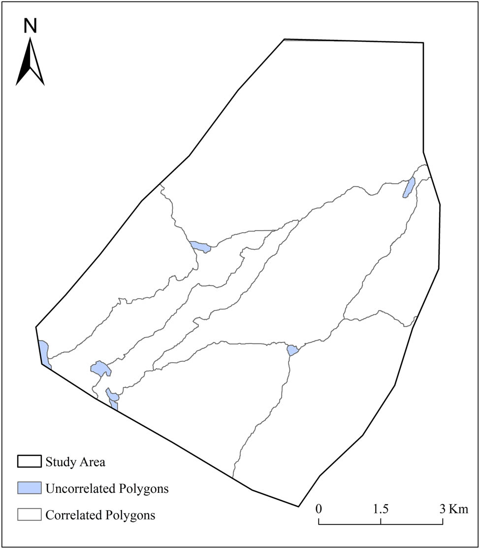
The hill boundary and ridge line data were read, respectively, and the corresponding numbers of elements are 437 and 8. Using the method proposed in Section 3.2.1, an attribute Id was assigned to each polygon of the hill boundary layer, and the results are shown in Table 5. Except for the polygons with an Id equal to −1 (uncorrelated polygons in Figure 6), polygons with the same Id were merged, and a total of eight correlated polygons (correlated polygons in Figure 6) were generated preliminarily.

Table 5

Number of polygons corresponding to each Id

Id	Number of polygons
−1	269
0	27
1	16
2	27
3	21
4	31
5	13
6	14
7	19

Figure 6

Hill boundaries obtained by correlating the separated polygons in Figure 5b using ridge lines.

4.1.3 Correlating separated polygons using valley lines

Attributes Fid, Line, and Dir were added to the uncorrelated polygons using the method proposed in Section 3.2.2. According to the rules proposed in Table 3, all eligible polygons were merged into the corresponding correlated polygons. The processing result of this section is shown in Figure 7, and seven uncorrelated polygons still exist after six iterations.

Figure 7

Hill boundaries obtained by correlating the uncorrelated polygons in Figure 6 using valley lines.

4.1.4 Correlating separated polygons without constraints

After successive correlations using ridge lines and valley lines, there were still a few ineligible polygons (as shown in Figure 7). Using the method proposed in Section 3.2.3, these polygons were recursively correlated following the longest common boundary principle until there were no uncorrelated polygons. The extracted eight hill boundaries are shown in Figure 8.

Figure 8

Hill boundaries obtained by merging the uncorrelated polygons in Figure 7 into adjacent correlated polygons following the longest common boundary principle. The base map is the hill shadow generated based on DEM.

4.2 Generating slope units

Based on the hill boundaries and ridge lines extracted in Section 4.1, the strike of each ridge line was calculated using the maximum frequency method proposed in Section 3.3 with the parameter T = 5. After extending and trimming the ridge lines (Figure 9), each hill boundary was divided into two slope units using the corresponding ridge line as the dividing line (Figure 10). The extracted 8 hill boundaries are divided into 16 slope units.

Figure 9

Comparison of the ridge lines before and after extending and trimming: (a) before extending and trimming and (b) after extending and trimming.

Figure 10

Slope units obtained by dividing each hill boundary into two parts using the corresponding ridge line.

4.3 Calculating the structural parameters of slopes

Using the method proposed in Section 3.4.1, the strike and dip direction of each slope were calculated according to the strike of the corresponding ridge line. Since the measured orientation data on the geological map is sparse (Figure 1c), the three-point and four-point methods are used to calculate the orientation of strata adaptively to obtain sufficient orientation data. The measured orientation and the calculated orientation are shown in Figure 11. Finally, based on the calculation results of the above steps, the structural parameters of each slope were calculated using the method proposed in Section 3.4.3.

Figure 11

Measured and calculated orientation data. The orange lines represent the boundaries of the main strata in the study area.

4.4 Classifying slopes

Based on the structural parameters calculated in Section 4.3, the slopes in the study area are classified according to the classification scheme shown in Table 2. Figure 12b shows the classification results, and Figure 12a shows the actual type of each slope identified by geological experts. The attributes of the slopes delineated and classified through this experiment are shown in Table 6.

Figure 12

Comparison of classified types and actual types of slopes. (a) The actual types of slopes. (b) The classified types of slopes. One slope is not successfully classified (the invalid value in (b)) due to its extremely long, narrow shape, which brings the result that it does not contain any measured or calculated orientation point.

Table 6

Values of attributes of each slope

Id	Classified types	Actual types	Slope surface orientation			Strata orientation			Plan-view area (m²)	Surface area (m²)	Shady/sunny
Id	Classified types	Actual types	Strike (°)	Dip direction (°)	Dip angle (°)	Strike (°)	Dip direction (°)	Dip angle (°)	Plan-view area (m²)	Surface area (m²)	Shady/sunny
1	Oblique	Oblique	54	144	19	43	313	74	10,706,800	16,271,280	Shady
2	Oblique	Oblique	54	324	17	37	307	58	10,436,500	14,839,411	Sunny
3	Oblique	Oblique	14	104	23	31	301	61	2,930,600	4,671,320	Shady
4	Oblique	Oblique	14	284	10	24	294	51	3,359,625	5,318,318	Sunny
5	Anti-dip	Anti-dip	44	134	21	35	305	62	2,295,550	3,125,234	Shady
6	Oblique	Dip	44	314	14	176	86	36	2,290,225	3,002,464	Sunny
7	Dip	Dip	44	134	18	39	129	66	2,516,150	3,161,602	Shady
8	—	Dip	44	314	20	—	—	—	963,050	1,251,114	Sunny
9	Dip	Dip	34	124	20	32	122	68	6,054,550	8,276,197	Shady
10	Dip	Dip	34	304	22	25	295	62	4,749,475	6,664,639	Sunny
11	Oblique	Oblique	54	144	34	96	6	36	1,070,075	1,737,088	Shady
12	Oblique	Oblique	54	324	18	9	279	55	2,764,525	3,987,319	Sunny
13	Dip	Dip	4	94	14	12	102	51	4,552,400	5,809,953	Shady
14	Dip	Dip	4	274	31	5	275	75	3,508,250	5,302,467	Sunny
15	Oblique	Dip	74	164	23	100	190	63	2,967,250	4,054,838	Shady
16	Oblique	Anti-dip	74	344	24	27	297	54	7,257,850	11,818,661	Sunny

Strikes and dip directions are represented in the form of azimuth. The slope with the Id value of 8 was not successfully classified due to its long, narrow shape, which brings the result that it does not contain any measured or calculated orientation point.

By comparing Figure 12a and b, it can be concluded that 12 slopes are correctly classified, 3 slopes are misclassified, and 1 slope is not successfully classified. As shown in Figure 12b, the slope adjacent to the anti-dip slope on the west side and the two slopes in the southeast corner of the study area are misclassified as oblique slopes. This is mainly because these slopes contain few or no measured orientation points and are steep in topography. These slopes lack orientation data, so their orientation can only be calculated based on DEM and geological maps. However, the terrain of these slopes is steep, which means that their DEM data contain large errors. Therefore, when calculating the orientation of these slopes, low-quality DEM may lead to incorrect calculation results. In addition, one slope (the invalid value in Figure 12b) is not successfully classified due to its extremely long, narrow shape, which brings the result that it does not contain any measured or calculated orientation point.

The performance of the method in this experiment can be summarized as follows: the correct classification rate is 75%, the false classification rate is 18.75%, and the missing classification rate is 6.25%.

5 Discussion

5.1 Factors affecting the method

5.1.1 Precision and richness of source data

During the process of extracting hill boundaries and terrain feature lines based on DEM data, the resolution of the DEM will affect the accuracy of the extracted results to a certain extent. On the other hand, the accuracy of the strata orientation calculation results is affected by the richness of the measured orientation data. Adequate measured data can accurately express the actual orientation of strata. In regions where the measured orientation data are scarce, it is necessary to calculate the strata orientation based on large-scale geological maps and DEM data, the accuracy of which is affected by the resolution of the DEM data and the level of detail of the geological maps. In general, high-precision source data and adequate measured orientation data can facilitate the application of the proposed method.

5.1.2 Area threshold used for eliminating tiny polygons

The polygons in the vector layer of hill boundaries extracted through hydrological analysis are relatively small and fragmented, and some of the extremely tiny polygons need to be eliminated. The elimination of tiny polygons is done by merging the polygons whose area is smaller than a specific area threshold into adjacent polygons, and the value of the area threshold is particularly critical in this process. If the threshold is too large, the final extracted hill boundaries may have excessive deformation and differ significantly from the actual hill boundaries. If the threshold is too small, there will still be excessive tiny polygons in the hill boundary layer, which will significantly increase the computational cost and time of the process of recursively correlating separated polygons using terrain feature lines. After multiple experiments, it has been proven that maintaining the ratio of the largest polygon’s area to the smallest polygon’s area at 20–100 is appropriate. Figure 13 shows the elimination results when applying different area thresholds.

Figure 13

Elimination results when applying different area thresholds: (a) Before eliminating. (b) Elimination results at an area threshold of 15,000 m². (c) Elimination results at an area threshold of 22,500 m². (d) Elimination results at an area threshold of 30,000 m².

5.1.3 Parameter T used for grouping azimuths

When generating slope units, the ridge lines need to be extended based on their strikes. To calculate the strike of a ridge line, every two adjacent points on the ridge line are used to generate a directed line segment. Next the azimuths of all directed line segments are calculated and sorted in reverse order by value. Then, the azimuths are grouped by dividing the azimuths with a difference less than the parameter T into the same group. And the value of T significantly influences the calculation of the strike of the ridge line. If the value of T is too large, the calculated strike will not be representative enough. If the value of T is too small, the calculated strike may deviate significantly from the real strike. When setting the value of the parameter T, the number of points contained by the ridge line should be considered. When the number of points forming the ridge line is around a few hundred or larger, it is appropriate to set the value of parameter T to around 5. When the number of points forming the ridge line is less than 100, the value of T should be appropriately increased.

5.2 Applicability of the method

First, sedimentary rocks with layered structures cover two-thirds of the land area, and many metamorphic rocks and volcanic rocks that have undergone sedimentation also have layered structural characteristics. Therefore, the method proposed in this work is applicable to regions where sedimentary rocks or metamorphic and volcanic rocks with layered structures are distributed.

Second, the proposed method aims to efficiently classify layered rock slopes, which determines that it mainly applies to mountainous and hilly areas. In addition, the proposed method extracts the hill boundaries based on DEM data. After eliminating the tiny polygons in the layer of hill boundaries extracted through hydrological analysis, the broken hill boundaries need to be correlated. And in the correlating process, ridge lines and valley lines are used as constraints to set the correlating rules. Consequently, this proposed method is applicable to mountainous and hilly areas and not to plain regions.

Finally, the proposed method is mainly applicable to providing references for large-scale urban and rural planning. Cities and villages in hilly areas often face frequent rock slope failures during development and construction [61], which often interrupts traffic flow and may cause severe damage to the lives and properties of nearby people [12,62,63,64]. Thus, for cities and villages in hilly areas, determining the stability of slopes and conducting landslide risk assessment are crucial for local planning and construction, which also has a strong social impact [4]. Therefore, during the development and construction of these regions, it is necessary to classify the slopes and evaluate their construction suitability.

In general, the method proposed in this work can meet the requirements of large-scale urban and rural planning and has better applicability in hilly regions mainly distributed with sedimentary rocks.

5.3 Significance of the proposed method

First, the morphology of the inverse DEM of a hill is consistent with a basin, so hill boundaries can be generated by extracting basin boundaries based on hydrological analysis of inverse DEM. The existing methods for extracting hill boundaries mainly follow this idea [65–67]. However, the results of watershed boundaries extraction are heavily affected by the area threshold values used [68–70], and the hill boundaries obtained by the above methods are usually very fragmented. Sergio et al. [71] tried to obtain drainage networks with a larger geographical scale using upscaling processes, which is suitable for alleviating this problem. From a new point of view, the proposed method uses terrain feature lines to correlate fragmented hill boundaries extracted by existing methods, through which intact and reasonable hill boundaries can be effectively generated. The extracted results are consistent with DEM data and can provide important references for geomorphological and hydrological studies.

Second, orientation data can be extracted from geological maps by obtaining a best-fit plane of more than three non-collinear points or by analyzing the moment of inertia of the points [72]. The former approach calculates a best-fit plane by planar regression [73–75] or statistical analysis [76] of data, which yields an average orientation for the point set. The latter approach is based on the concept that the axis of maximum moment of inertia represents the pole to the best-fit plane through the set of points [72,77]. Following the idea of plane fitting, the method in this study adaptively chooses either the three-point or four-point method for orientation calculation. This adaptive orientation calculation method can reduce errors to some extent [59], which gives it unique research value.

6 Conclusion

This study proposes a semi-automated classification method for layered rock slopes based on relatively easy-to-access DEM data and geological maps. To address the problem that the hill boundaries extracted through hydrological analysis are fragmented, this work uses terrain feature lines to correlate the extracted polygons, which can generate intact hill boundaries. To solve the problem that the measured orientation data in the application region may be insufficient, this work calculates strata orientation based on DEM and geological maps, which effectively supports the classification of layered rock slopes in areas where the measured orientation data are scarce. Moreover, this method’s high degree of automation supports the application of large-scale urban and rural planning and landslide hazard assessment.

The case study in the northern region of Mount Lu shows that the proposed method can effectively classify layered rock slopes over large areas with sparse measured orientation data. The precision and richness of the source data will affect the application effect of the proposed method to a certain extent. Moreover, the accuracy of the proposed method is mainly affected by the area threshold used to eliminate tiny polygons in the vector layer of hill boundaries and the grouping parameter used to calculate the strikes of ridge lines. Compared with the existing manual or semi-automated classification methods, the method proposed in this study is not influenced by subjective factors and significantly improves the degree of automation, which can meet the requirements of classification of layered rock slopes over large areas. In addition, the classification results of layered rock slopes can provide essential references for urban and rural planning and valuable information for stability analysis of layered rock slopes.

Similarly, for rock slopes with other structural characteristics, the idea of this method can be applied to develop classification schemes based on their structural features and then calculate their structural parameters to classify slopes efficiently. The hill boundary extraction method combining terrain feature lines can provide meaningful references for automated boundary extraction of other geomorphic entities.

# These authors contributed equally to this work.

Funding information: This study was supported by the National Natural Science Foundation of China (Project Nos. 41971068 and 41771431) and Jinan Science and Technology Innovation Development Plan Project (Project No. 202131001).
Author contributions: Hao Shang is the primary author of the article. Da-Hai Wang and Meng-Yuan Li developed the main modules of the prototype system and are the key contributors to the methodology. Yu-Hong Ma developed partial modules of the prototype system. Shi-Peng Yang prepared the experimental data. An-Bo Li conceived the original idea and offered supervision. All authors have read and agreed to the published version of the manuscript.
Conflict of interest: The authors declare no conflict of interest.

References

[1] Crozier MJ. Environmental Geology. Dordrecht: Kluwer Academic Publishers; 1999. p. 561–2. 10.1007/1-4020-4494-1_304.Search in Google Scholar

[2] Dai FC, Lee CF. Landslide characteristics and slope instability modeling using GIS, Lantau Island, Hong Kong. Geomorphology. 2002;42(3–4):213–28. 10.1016/S0169-555X(01)00087-3.Search in Google Scholar

[3] Lee S, Choi J. Landslide susceptibility mapping using GIS and the weight-of-evidence model. Int J Geogr Inf Sci. 2004;18(8):789–814. 10.1080/13658810410001702003.Search in Google Scholar

[4] Sassa K, Wang G, Fukuoka H, Wang F, Ochiai T, Sugiyama M, et al. Landslide risk evaluation and hazard zoning for rapid and long-travel landslides in urban development areas. Landslides. 2004;1(3):221–35. 10.1007/s10346-004-0028-y.Search in Google Scholar

[5] Guzzetti F, Reichenbach P, Cardinali M, Galli M, Ardizzone F. Probabilistic landslide hazard assessment at the basin scale. Geomorphology. 2005;72(1–4):272–99. 10.1016/j.geomorph.2005.06.002.Search in Google Scholar

[6] Scaioni M, Longoni L, Melillo V, Papini M. Remote sensing for landslide investigations: an overview of recent achievements and perspectives. Remote Sens. 2014;6(10):9600–52. 10.3390/rs6109600.Search in Google Scholar

[7] Wubalem A. Modeling of landslide susceptibility in a part of Abay Basin, northwestern Ethiopia. Open Geosci. 2020;12(1):1440–67. 10.1515/geo-2020-0206.Search in Google Scholar

[8] Zhao H, Tian WP, Li J, Ma BC. Hazard zoning of trunk highway slope disasters: a case study in northern Shaanxi, China. Bull Eng Geol Env. 2018;77(4):1355–64. 10.1007/s10064-017-1178-1.Search in Google Scholar

[9] Su H, Li J, Cao J, Wen Z. Macro-comprehensive evaluation method of high rock slope stability in hydropower projects. Stoch Env Res Risk Assess. 2014;28(2):213–24. 10.1007/s00477-013-0742-x.Search in Google Scholar

[10] Li XZ, Tan RZ, Gao Y. Modification of slope stability probability classification and its application to rock slopes in hydropower engineering regions. Geol Croat. 2019;72:71–80. 10.4154/gc.2019.20.Search in Google Scholar

[11] Basahel H, Mitri H. Application of rock mass classification systems to rock slope stability assessment: A case study. J Rock Mech Geotech Eng. 2017;9(6):993–1009. 10.1016/j.jrmge.2017.07.007.Search in Google Scholar

[12] Dakssa LM. Some aspects of rock slopes stabilization in urban areas in Sultanate of Oman. 3rd Mec International Conference on Big Data and Smart City (icbdsc). New York: Ieee; 2016; 2016. p. 244–9.10.1109/ICBDSC.2016.7460375Search in Google Scholar

[13] Robertson AM. Estimating weak rock strength. SME Annual Meeting. Phoenix; 1988. p. 1–5.10.1016/0892-6875(88)90011-8Search in Google Scholar

[14] Romana MR. Rock testing and site characterization. Oxford: Pergamon; 1993. p. 575–600. 10.1016/B978-0-08-042066-0.50029-X.Search in Google Scholar

[15] Shuk T. Key elements and applications of the natural slope methodology (NSM) with some emphasis on slope stability aspects. 4th South American Congress on Rock Mechanics; 1994.Search in Google Scholar

[16] Chen Z. Recent developments in slope stability analysis. 8th ISRM Congress; 1995.Search in Google Scholar

[17] Hack R, Price D, Rengers N. A new approach to rock slope stability – a probability classification (SSPC). Bull Eng Geol Env. 2003;62(2):167–84. 10.1007/s10064-002-0155-4.Search in Google Scholar

[18] Tomás R, Delgado J, Serón JB. Modification of slope mass rating (SMR) by continuous functions. Int J Rock Mech Min Sci. 2007;44(7):1062–9. 10.1016/j.ijrmms.2007.02.004.Search in Google Scholar

[19] Bar N, Barton NR. Empirical Slope design for hard and soft rocks using Q-slope. 50th U.S. Rock Mechanics/Geomechanics Symposium. Houston, Texas; 2016.Search in Google Scholar

[20] Wu A, Zhao W, Zhang Y, Fu X. A detailed study of the CHN-BQ rock mass classification method and its correlations with RMR and Q system and Hoek-Brown criterion. Int J Rock Mech Min Sci. 2023;162:105290. 10.1016/j.ijrmms.2022.105290.Search in Google Scholar

[21] Li XZ, Xu Q. Application of the SSPC method in the stability assessment of highway rock slopes in the Yunnan province of China. Bull Eng Geol Env. 2016;75(2):551–62. 10.1007/s10064-015-0792-z.Search in Google Scholar

[22] Lin CH, Lin ML, Peng HR, Lin HH. Framework for susceptibility analysis of layered rock slopes considering the dimensions of the mapping units and geological data resolution at various map scales. Eng Geol. 2018;246:310–25. 10.1016/j.enggeo.2018.10.004.Search in Google Scholar

[23] Terzaghi K. Rock defects and loads on tunnel supports. Rock Tunneling with Steel Supports; 1946.Search in Google Scholar

[24] Bieniawski ZT. Engineering classification of jointed rock masses. Trans S Afr Inst Civ Engrs. 1973;15(12):335–43.Search in Google Scholar

[25] Barton N, Lien R, Lunde J. Engineering classification of rock masses for the design of tunnel support. Rock Mech. 1974;6(4):189–236. 10.1007/BF01239496.Search in Google Scholar

[26] Laubscher DH. A geomechanics classification system for the rating of rock mass in mine design. J S Afr Inst Min Metall. 1990;90(10):257–73. 10.10520/AJA0038223X_1954.Search in Google Scholar

[27] Jorda-Bordehore L. Application of Q (slope) to assess the stability of rock slopes in Madrid Province, Spain. Rock Mech Rock Eng. 2017;50(7):1947–57. 10.1007/s00603-017-1211-5v.Search in Google Scholar

[28] Arab PB, Vieira L, de Siqueira AF. A comparison between SMR and SSPC classification systems for the assessment of rock slope stability in the context of Pelotas Batholith, Cangucu, Rio Grande do Sul, Brazil. J South Am Earth Sci. 2021;110:103419. 10.1016/j.jsames.2021.103419.Search in Google Scholar

[29] Jakubec J, Laubscher DH. The MRMR Rock Mass Rating Classification System in Mining Practice. 3rd International Conference and Exhibition on Mass Mining. Brisbane, Australia: 2000. p. 413–21.Search in Google Scholar

[30] Jakubec J, Esterhuizen GS. Use of the mining rock mass rating (MRMR) classification: Industry experience. International Workshop on Rock Mass Classification in Underground Mining; 2007.Search in Google Scholar

[31] Panzhin AA, Kharisov TF, Kharisova OD. Substantiation of stable pitwall parameters based on the mining rock mass rating. J Min Sci. 2019;55(4):522–30. 10.1134/S1062739119045867.Search in Google Scholar

[32] Siddique T, Masroor Alam M, Mondal MEA, Vishal V. Slope mass rating and kinematic analysis of slopes along the national highway-58 near Jonk, Rishikesh, India. J Rock Mech Geotech Eng. 2015;7(5):600–6. 10.1016/j.jrmge.2015.06.007.Search in Google Scholar

[33] Azarafza M, Akgun H, Asghari-Kaljahi E. Assessment of rock slope stability by slope mass rating (SMR): A case study for the gas flare site in Assalouyeh. South Iran Geomech Eng. 2017;13(4):571–84. 10.12989/GAE.2017.13.4.571.Search in Google Scholar

[34] Jorda-Bordehore L, Bar N, González MC, Guill AR, Jover RT. Stability assessment of rock slopes using empirical approaches: comparison between Slope Mass Rating and Q-Slope. 14th International Congress of Energe and Mineral Resources, Slope Stability, Seville, Spain; 2018.Search in Google Scholar

[35] Akram MS, Ahmed L, Farooq S, Ahad MA, Zaidi SMH, Khan M, et al. Geotechnical evaluation of rock cut slopes using basic Rock Mass Rating (RMRbasic), Slope Mass Rating (SMR) and Kinematic Analysis along Islamabad Muzaffarabad Dual Carriageway (IMDC), Pakistan. J Biodivers Environ Sci. 2018;13:297–306.Search in Google Scholar

[36] Hamzeh MAS. Application of Fuzzy logic to investigate Slope Mass Rating (SMR) in Khoy open-pit mining projects. Geotech Geol. 2019;15(1):283–7.Search in Google Scholar

[37] Triana K, Hermawan K. Slope mass rating-based analysis to assess rockfall hazard on Yogyakarta Southern Mountain, Indonesia. Geoenviron Disasters. 2020;7(1):24. 10.1186/s40677-020-00164-w.Search in Google Scholar

[38] Azarafza M, Nanehkaran YA, Rajabion L, Akgün H, Rahnamarad J, Derakhshani R, et al. Application of the modified Q-slope classification system for sedimentary rock slope stability assessment in Iran. Eng Geol. 2020;264:105349. 10.1016/j.enggeo.2019.105349.Search in Google Scholar

[39] Matsimbe J. Comparative application of photogrammetry, handmapping and android smartphone for geotechnical mapping and slope stability analysis. Open Geosci. 2021;13(1):148–65. 10.1515/geo-2020-0213.Search in Google Scholar

[40] Zhu H, Azarafza M, Akgun H. Deep learning-based key-block classification framework for discontinuous rock slopes. J Rock Mech Geotech Eng. 2022;14(4):1131–9. 10.1016/j.jrmge.2022.06.007.Search in Google Scholar

[41] Sheng D, Yu J, Tan F, Tong D, Yan T, Lv J. Rock mass quality classification based on deep learning: A feasibility study for stacked autoencoders. J Rock Mech Geotech Eng. 2023;15(7):1749–58. 10.1016/j.jrmge.2022.08.006.Search in Google Scholar

[42] Brousset J, Pehovaz H, Quispe G, Raymundo C, Moguerza JM. Rock mass classification method applying neural networks to minimize geomechanical characterization in underground Peruvian mines. Energy Rep. 2023;9:376–86. 10.1016/j.egyr.2023.05.246.Search in Google Scholar

[43] Jin DL. Engineering geologic classification of slopes for water resources and hydropower projects. Northwest Hydropower. 2000;2:10–5 (in Chinese).Search in Google Scholar

[44] Zhou DP, Zhong W, Yang T. Stability analysis of rock slope based on slope structures. Chin J Rock Mech Eng. 2008;4:687–95 (in Chinese).Search in Google Scholar

[45] Stead D, Wolter A. A critical review of rock slope failure mechanisms: The importance of structural geology. J Struct Geol. 2015;74:1–23. 10.1016/j.jsg.2015.02.002.Search in Google Scholar

[46] Stead D, Donati D, Wolter A, Sturzenegger M. Application of Remote Sensing to the Investigation of Rock Slopes: Experience Gained and Lessons Learned. ISPRS Int Geo-Inf. 2019;8(7):296. 10.3390/ijgi8070296.Search in Google Scholar

[47] Zheng D, Zhou H, Zhou H, Liu F, Chen Q, Wu Z. Effects of Slope Angle on Toppling Deformation of Anti-Dip Layered Rock Slopes: A Centrifuge Study. Appl Sci-Basel. 2022;12(10):5084. 10.3390/app12105084.Search in Google Scholar

[48] Dong M, Zhang F, Yu C, Lv J, Zhou H, Li Y, et al. Influence of a dominant fault on the deformation and failure mode of anti-dip layered rock Slopes. KSCE J Civ Eng. 2022;26(8):3430–9. 10.1007/s12205-022-1852-0.Search in Google Scholar

[49] Li AB, Chen Y, Lü GN, Zhu AX. Automatic detection of geological folds using attributed relational graphs and formal grammar. Comput Geosci. 2019;127:75–84. 10.1016/j.cageo.2019.03.006.Search in Google Scholar

[50] Cun JF. Failure mechanism and stability appraisal theory study on layered rock slope in karst region. Master. Guizhou University; 2007 (in Chinese).Search in Google Scholar

[51] Guo BB, Shu JS, Shu YQ, Lü JX. Study on slope engineering geological model and slope stability of flat rock strata. China Min Mag. 2012;21(2):104–7 (in Chinese).Search in Google Scholar

[52] Sun GZ. Geological models and classification of rock slopes. Engineering Geology and Geological Engineering. Beijing: Seismological Press; 1993. p. 171–2 (in Chinese).Search in Google Scholar

[53] Zhong T, Tang GA, Zhou Y, Li RY, Zhang W. Method of extracting surface peaks based on reverse DEMs. Bull Surveying Mapp. 2009;4:35–7 (in Chinese) .Search in Google Scholar

[54] O’Callaghan JF, Mark DM. The extraction of drainage networks from digital elevation data. Computer Vision, Graphics, Image Process. 1984;28(3):323–44. 10.1016/S0734-189X(84)80011-0.Search in Google Scholar

[55] Jenson SK, Domingue JO. Extracting topographic structure from digital elevation data for geographic information system analysis. Photogramm Eng Rem S. 1988;54(11):1593–600.Search in Google Scholar

[56] Xiao F, Zhang BP, Ling F, Xue HP, Du Y, Wu HZ. DEM based auto-extraction of geomorphic units. Geogr Res. 2008;27(2):459–66 (in Chinese) .Search in Google Scholar

[57] Alvioli M, Marchesini I, Reichenbach P, Rossi M, Ardizzone F, Fiorucci F, et al. Automatic delineation of geomorphological slope units with r.slopeunits v1.0 and their optimization for landslide susceptibility modeling. Geosci Model Dev. 2016;9(11):3975–91. 10.5194/gmd-9-3975-2016.Search in Google Scholar

[58] Wang F, Xu P, Wang C, Wang N, Jiang N. Application of a GIS-based slope unit method for landslide susceptibility mapping along the Longzi River, Southeastern Tibetan Plateau, China. ISPRS Int Geo-Inf. 2017;6(6):172. 10.3390/ijgi6060172.Search in Google Scholar

[59] Liu XY, Li AB, Chen H, Men YQ, Huang YL. 3D modeling method for dome structure using digital geological map and DEM. ISPRS Int J Geo-Inf. 2022;11(6):339. 10.3390/ijgi11060339.Search in Google Scholar

[60] Wang H, Hu GH, Ma JF, Wei H, Li SJ, Tang GA, et al. Classifying Slope Unit by Combining Terrain Feature Lines Based on Digital Elevation Models. Land. 2023;12(1):193. 10.3390/land12010193.Search in Google Scholar

[61] Sun X, Chen J, Bao Y, Han X, Zhan J, Peng W. Landslide susceptibility mapping using logistic regression analysis along the Jinsha River and its tributaries close to Derong and Deqin County, Southwestern China. ISPRS Int Geo-Inf. 2018;7(11):438. 10.3390/ijgi7110438.Search in Google Scholar

[62] Hoelbling D, Fuereder P, Antolini F, Cigna F, Casagli N, Lang S. A Semi-Automated Object-Based Approach for Landslide Detection Validated by Persistent Scatterer Interferometry Measures and Landslide Inventories. Remote Sens. 2012;4(5):1310–36. 10.3390/rs4051310.Search in Google Scholar

[63] Tavakkoli Piralilou S, Shahabi H, Jarihani B, Ghorbanzadeh O, Blaschke T, Gholamnia K, et al. Landslide detection using multi-scale image segmentation and different machine learning models in the higher himalayas. Remote Sens. 2019;11(21):2575. 10.3390/rs11212575.Search in Google Scholar

[64] Anis Z, Wissem G, Vali V, Smida H, Essghaier GM. GIS-based landslide susceptibility mapping using bivariate statistical methods in North-western Tunisia. Open Geosci. 2019;11(1):708–26. 10.1515/geo-2019-0056.Search in Google Scholar

[65] Wang T. A New Algorithm for Extracting Drainage Networks from Gridded DEMs. In: Buchroithner M, Prechtel N, Burghardt D, editors. Cartography from Pole to Pole: Selected Contributions to the XXVIth International Conference of the ICA, Dresden 2013. Berlin, Heidelberg: Springer; 2014. p. 335–53. 10.1007/978-3-642-32618-9_24.Search in Google Scholar

[66] Qu G, Su D, Lou Z. A new algorithm to automatically extract the drainage networks and catchments based on triangulation irregular network digital elevation model. J Shanghai Jiaotong Univ (Sci). 2014;19(3):367–77. 10.1007/s12204-014-1511-9.Search in Google Scholar

[67] Siddiqui S, Castaldini D, Soldati M. DEM-based drainage network analysis using steepness and Hack SL indices to identify areas of differential uplift in Emilia–Romagna Apennines, northern Italy. Arab J Geosci. 2016;10(1):3. 10.1007/s12517-016-2795-x.Search in Google Scholar

[68] Gautam S, Dahal V, Bhattarai R. Impacts of DEM source, resolution and area threshold values on SWAT generated stream network and streamflow in two distinct Nepalese catchments. Env Process. 2019;6(3):597–617. 10.1007/s40710-019-00379-6.Search in Google Scholar

[69] Munoth P, Goyal R. Effects of DEM source, spatial resolution and drainage area threshold values on hydrological modeling. Water Resour Manag. 2019;33(9):3303–19. 10.1007/s11269-019-02303-x.Search in Google Scholar

[70] Datta S, Karmakar S, Mezbahuddin S, Hossain MM, Chaudhary BS, Hoque ME, et al. The limits of watershed delineation: implications of different DEMs, DEM resolutions, and area threshold values. Hydrol Res. 2022;53(8):1047–62. 10.2166/nh.2022.126.Search in Google Scholar

[71] Rosim S, Ortiz, JdeO, de Freitas Oliveira JR, Jardim AC, Abreu ES. Drainage network definition for low resolution DEM obtained from drainage network extracted from high resolution DEM using upscaling processes. In: Lollino G, Arattano M, Rinaldi M, Giustolisi O, Marechal JC, Grant GE, editors. Engineering Geology For Society And Territory, River Basins, Reservoir Sedimentation And Water Resources. Cham: Springer International Publishing Ag: 2015;Vol: 3, p. 271–4. 10.1007/978-3-319-09054-2_56.Search in Google Scholar

[72] Fernandez O. Obtaining a best fitting plane through 3D georeferenced data. J Struct Geol. 2005;27(5):855–8. 10.1016/j.jsg.2004.12.004.Search in Google Scholar

[73] Rauch A, Sartori M, Rossi E, Baland P, Castelltort S. Trace Information Extraction (TIE): A new approach to extract structural information from traces in geological maps. J Struct Geol. 2019;126:286–300. 10.1016/j.jsg.2019.06.007.Search in Google Scholar

[74] Allmendinger RW. GMDE: Extracting quantitative information from geologic. Geosphere. 2020;16(6):1495–507. 10.1130/GES02253.1.Search in Google Scholar

[75] Jessell M, Ogarko V, de Rose Y, Lindsay M, Joshi R, Piechocka A, et al. Automated geological map deconstruction for 3D model construction using map2loop 1.0 and map2model 1.0. Geosci Model Dev. 2021;14(8):5063–92. 10.5194/gmd-14-5063-2021.Search in Google Scholar

[76] Thiele ST, Grose L, Cui T, Cruden AR, Micklethwaite S. Extraction of high-resolution structural orientations from digital data: A Bayesian approach. J Struct Geol. 2019;122:106–15. 10.1016/j.jsg.2019.03.001.Search in Google Scholar

[77] Nibourel L, Morgenthaler J, Grazioli S, Schumacher I, Schlafli S, Galfetti T, et al. Automated extraction of orientation and stratigraphic thickness from geological maps. J Struct Geol. 2023;172:104865. 10.1016/j.jsg.2023.104865.Search in Google Scholar

Received: 2023-05-06

Revised: 2023-07-17

Accepted: 2023-08-08

Published Online: 2023-08-21

This work is licensed under the Creative Commons Attribution 4.0 International License.

Articles in the same Issue

https://doi.org/10.1515/geo-2022-0526

Keywords for this article

layered rock slope; classification; structural characteristics; DEM; geological map

Creative Commons

BY 4.0