Minimal universal laser network model: Synchronization, extreme events, and multistability
-
Mahtab Mehrabbeik


Abstract
The synchronization of chaotic systems has garnered considerable attention across various fields, including neuroscience and physics. Particularly in these domains, synchronizing physical systems such as laser models is crucial for secure and rapid information transmission. Consequently, numerous studies investigate the synchronizability of different laser networks by establishing logical network frameworks. In this study, we employed a minimal universal laser (MUL) model designed to capture the essential dynamics of an actual laser model within just three dimensions. Within the network model of MUL systems, we introduced the linear diffusive function of neighboring nodes’ fast variables into the feedback term of the lasers, with models arranged in a global network structure. Our examination of synchronization within the constructed MUL network utilized master stability functions and the time-averaged synchronization error index. The findings suggest that while the network fails to achieve complete synchrony, it exhibits various synchronization phenomena, including cluster synchronization, chimera states, extreme events, and multistability. These results shed light on the complex dynamics underlying the synchronization of chaotic systems in networked environments, offering insights relevant to numerous applications across diverse fields.
1 Introduction
Among the various collective dynamics that can emerge in coupled dynamical systems featured by complex networks – defined as a set of dynamical nodes connected through links in a specific structure and coupling scheme [1] – synchronization holds a prominent position. As a fundamental concept, synchronization denotes a state wherein all oscillators in a network exhibit identical temporal evolutions [2]. Consequently, the solution of the connected system is not only consistent in state space but also in the time domain. This specific state is referred to as full or complete synchronization, while synchronization encompasses a broader class of collective dynamics, indicating the emergence of coherence among the dynamical nodes [3]. Different synchronization patterns can be defined based on the level of coherence observed. For instance, cluster synchronization describes a state where the solutions of connected oscillators converge to different attractors, forming clusters with full coherence [4]. Another notable subgroup of synchronization is the chimera state, wherein the coexistence of one or a few coherent clusters with an incoherent one is observed [5,6]. Additionally, various other types of synchronization include phase synchronization [7], lag synchronization [8], solitary state [9], generalized synchronization [10], and relay synchronization [11]. Each of these synchronization patterns provides insight into the intricate dynamics of coupled dynamical systems on complex networks.
Synchronization is a concept extensively studied across various fields, with particular significance in neuroscience [12–14] and physics [15–17]. In neuroscience, modeling brain networks involves intricate neuronal models and synaptic pathways. These models are crucial for understanding how synchronization manifests within the brain’s complex network architecture [18–20]. In the realm of physics, certain physical systems play a vital role in the study of synchronization. Among these, laser systems are particularly noteworthy, representing a cornerstone of nonlinear dynamics and chaos theory in real-world applications. Numerous versions of laser systems have been proposed in the literature, each offering unique insights into the dynamics of synchronized systems. For instance, Haken introduced the single-mode laser model [21], while Agrawal developed a mathematical model for semiconductor lasers [22]. Additionally, Ciofini et al. introduced the four-level CO2 laser model [23], while Meucci et al. proposed the minimal universal laser (MUL) model [24] and a modulated laser system [25]. As highlighted by Uchida et al., the synchronization of chaotic laser models is crucial as it facilitates information communication in both analog and digital forms [26]. Recognizing this significance, numerous studies have delved into examining the synchronization of networked laser systems by proposing physically meaningful coupling schemes. For instance, Sugawara et al. [27] and Mariño et al. [28] explored master-slave laser network configurations. DeShazer et al. [29] and Hillbrand et al. [30] focused on phase synchronization in coupled laser systems. Lag synchronization in an undirected ring network of laser systems was investigated by Mihana et al. [31]. Zhang et al. [32] documented chimera state and cluster synchronization exhibited by delay-coupled laser systems. Similarly, Chembo Kouomou and Woafo [33] found cluster synchronization in a two-dimensional laser network, while Röhm et al. [34] reported a chimera state when the connections of the laser systems involve delays. The phenomenon of cluster synchronization has also been observed in a nonlocally coupled semiconductor laser system, as noted by Kazakov et al. [35]. Additionally, Roy et al. [36] investigated the synchronization of hyperchaotic non-autonomous optically modulated CO2 laser systems, focusing on the effects of ring and star coupling configurations on synchronization cost. Mehrabbeik et al. [15] also investigated the multistability of a modulated laser network and reported the emergence of cluster synchronization, chimera states, and solitary states within the network. These studies collectively contribute to our understanding of the synchronization phenomena in laser systems and their implications for information processing and communication.
Extreme events represent a category of dynamical properties characterized by the sudden emergence of high-amplitude oscillations or fluctuations within a system. These fluctuations are often undesired and unpredictable, posing significant challenges in their management [37,38]. Extreme events can manifest either in the dynamics of an isolated system [39,40] or in the behavior of coupled systems [41–43]. Multistability is another crucial dynamical property observed in both isolated [25,44] and coupled models [15,45]. It denotes a condition wherein the system lacks a unique solution, resulting in the network’s solution being contingent upon the selection of initial states [46]. Extreme multistability [47,48] and megastability [49,50] represent special cases of multistability wherein the system demonstrates an infinite number of solutions. In extreme multistability, these solutions are uncountable, while in megastability, they are countable.
This article explores the synchronization dynamics of the MUL laser model, given its capability to exhibit chaos and adhere to laser dynamical properties within a low-dimensional framework. Following the introduction of the MUL laser model, Section 2 delves into the chaotic dynamics of the MUL model through bifurcation and Lyapunov analysis. In this section, we also introduce a suitable coupling scheme and global configuration alongside the formulation of the MUL network model. Moving to Section 3, we conduct a stability analysis of the synchronization state of the constructed network, employing both analytical methods and numerical approaches for validation. Furthermore, a comprehensive analysis is undertaken to elucidate the prominent synchronization patterns observed within the network. Finally, Section 4 provides a conclusion, summarizing the key findings and implications of the study.
2 Model
The CO2 laser model’s unique characteristics were captured in a three-dimensional chaotic model introduced in the study by Meucci et al. [24], aligning closely with a laser system’s physics and inherent properties. This proposed laser model is mathematically described as follows:
where the variables
Under the transformation
With

Dynamical analysis of the MUL system as a function of the parameter
Figure 1 illustrates that the MUL model transitions into the chaotic region (at

Trajectory (left panels) and temporal pattern (right panels) of the chaotic attractors of the MUL model for (a, b)
It is worth mentioning that within the chaotic region, various periodic windows can be discerned. The most expansive ones, located within the first and second chaotic regimes, are extended between
To delve into the synchronization dynamics of the MUL model, we must examine the coupled models within a predetermined network framework. Coupling the MUL models involves integrating the linear diffusive function of the fast variable from neighboring nodes into the feedback mechanism. Consequently, the structure of the MUL network model can be outlined as follows:
For every node indexed by
In the forthcoming section, we explore the synchronization state of Network (4) under homoclinic chaos conditions (with parameters set as identical to those in Figure 2(c) and (d)), leveraging insights from both analytical approaches and numerical simulations.
3 Synchronization analysis
In the synchronization state, all nodes exhibit an identical simultaneous temporal pattern, meaning
where

Analytical (left panel) and numerical (right panel) analysis of the MUL network synchronization with global coupling scheme and
In Eq. (6),
Although the MUL network model cannot achieve complete synchrony, our comprehensive analysis of the collective dynamics of Network (4) reveals intriguing monostable or multistable synchronization patterns. For instance, at lower values of
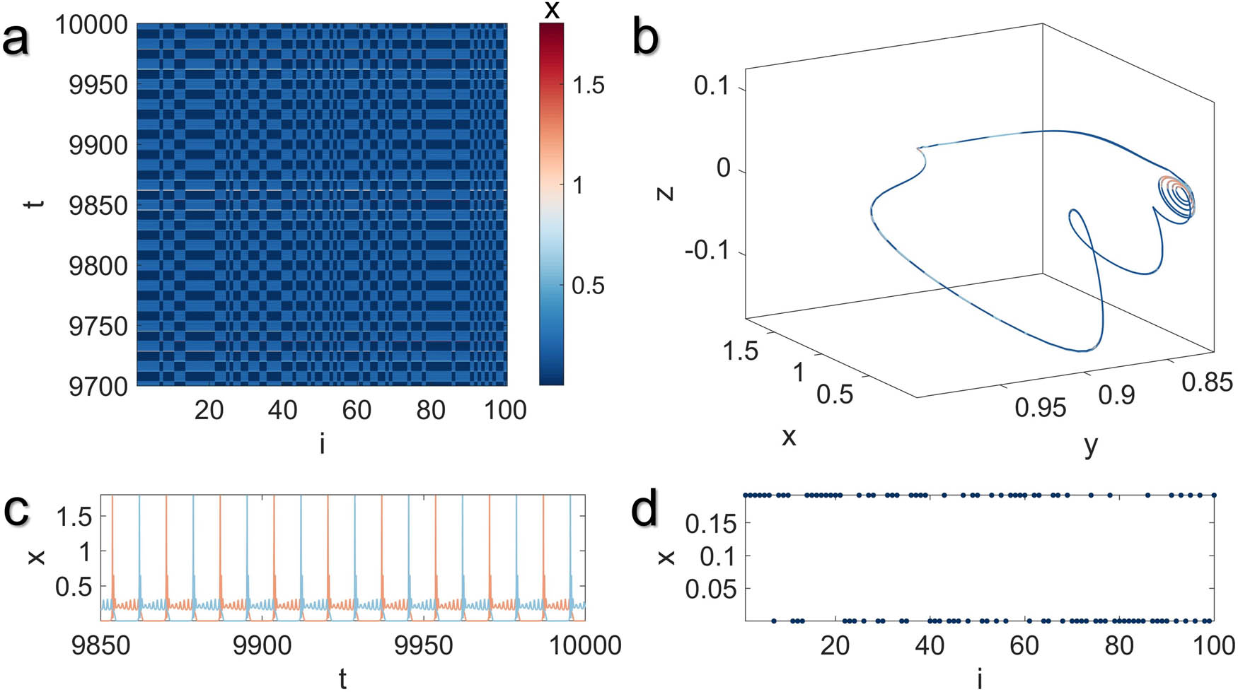
Illustration of the monostable two-cluster synchronization state in the MUL network model with global coupling structure for
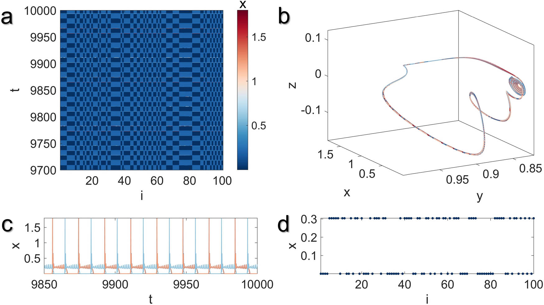
Illustration of the multistable two-cluster synchronization state in the MUL network model with global coupling structure for
Figures 6 and 7 depict how the rise in the value of
where
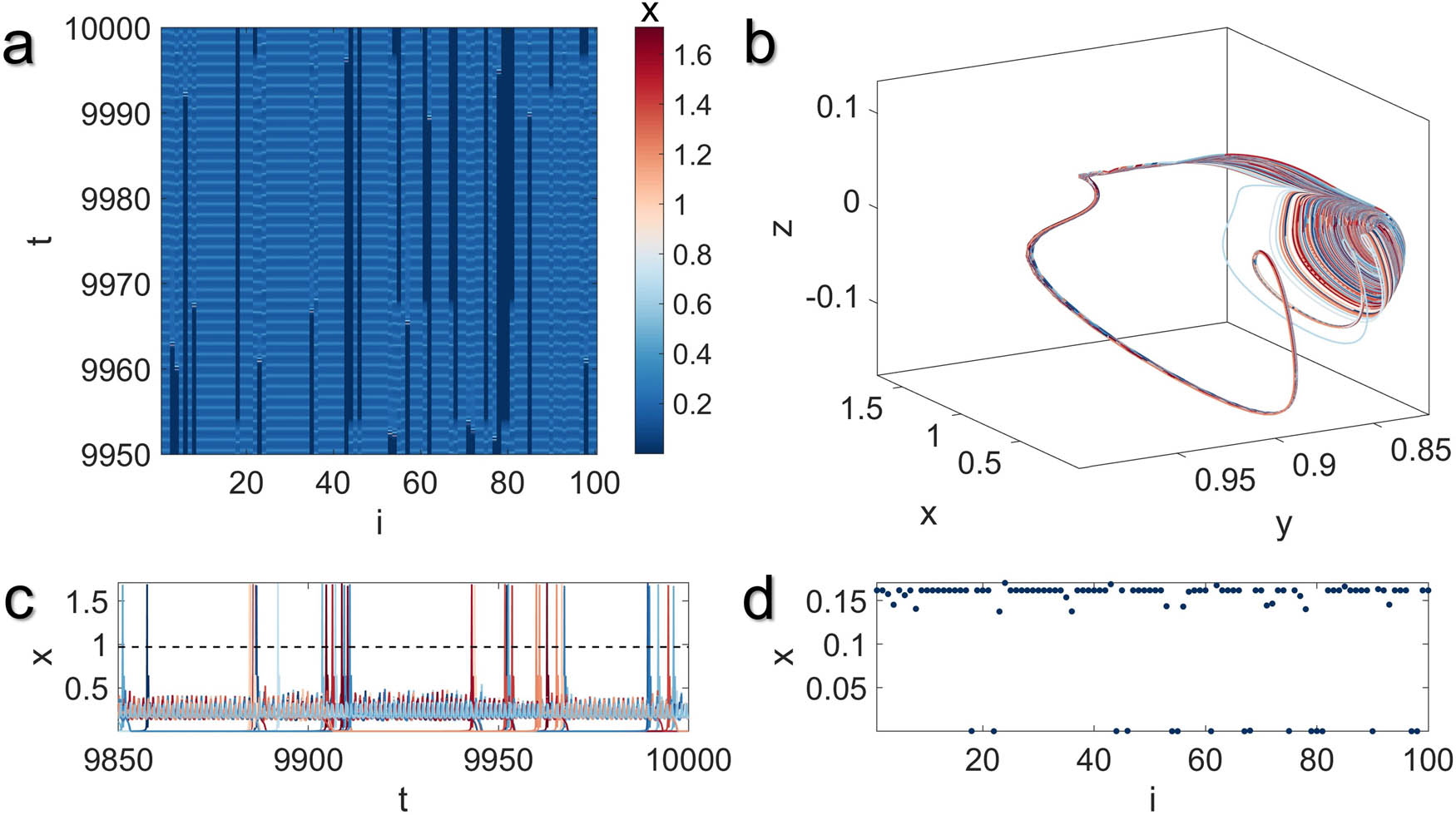
Illustration of the multistable chimera state with extreme events in the MUL network model with global coupling structure for
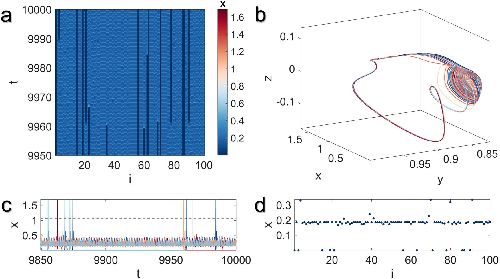
Illustration of the multistable chimera state with extreme events in the MUL network model with global coupling structure for
According to Figures 8 and 9, as
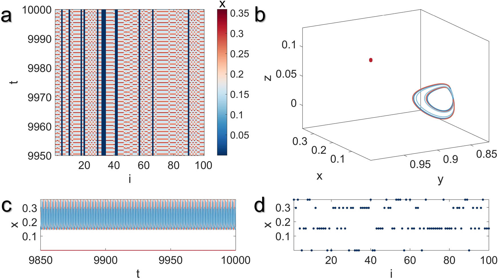
Illustration of the multistable four-cluster synchronization state in the MUL network model with global coupling structure for
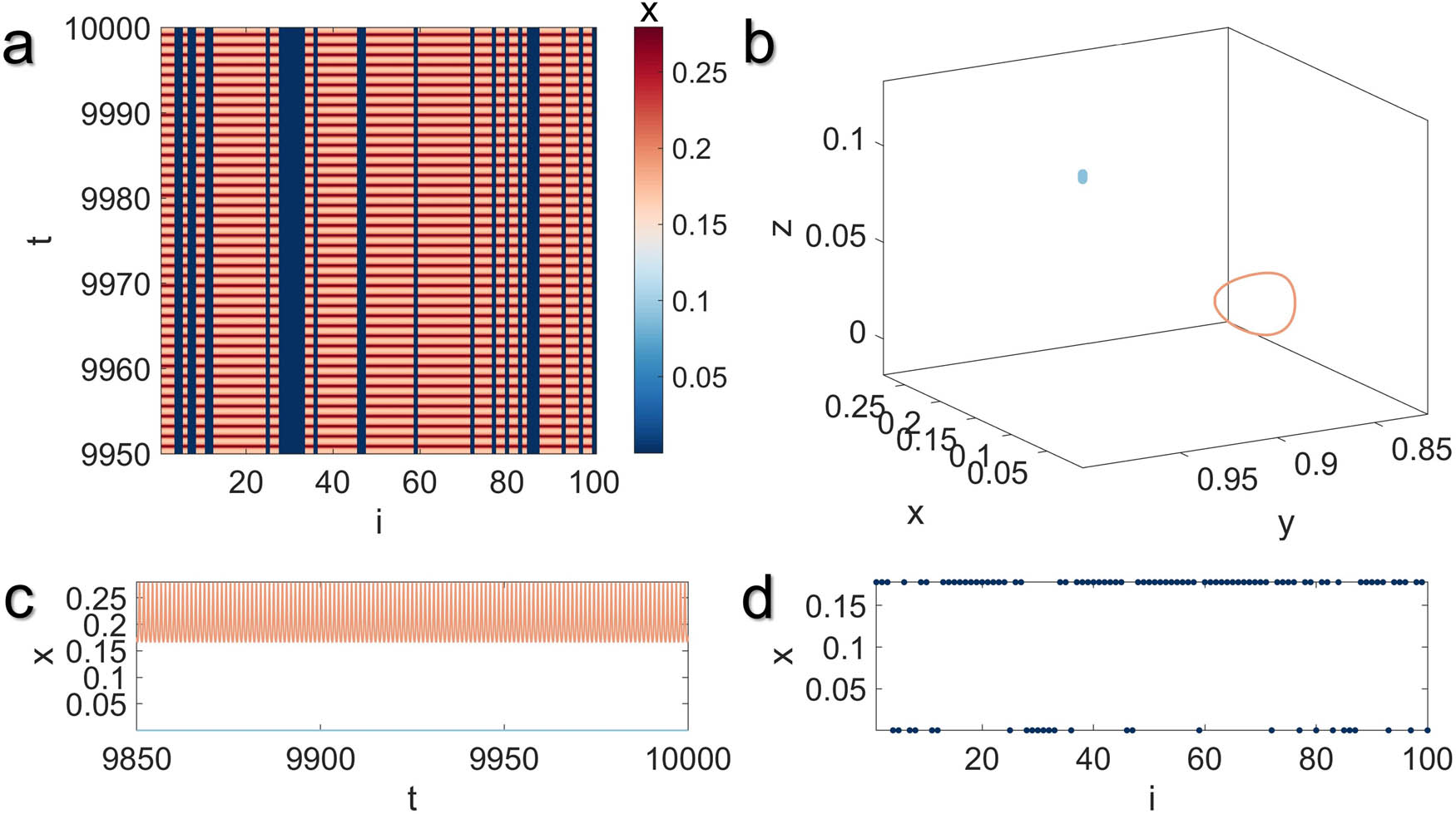
Illustration of the multistable two-cluster synchronization state in the MUL network model with global coupling structure for
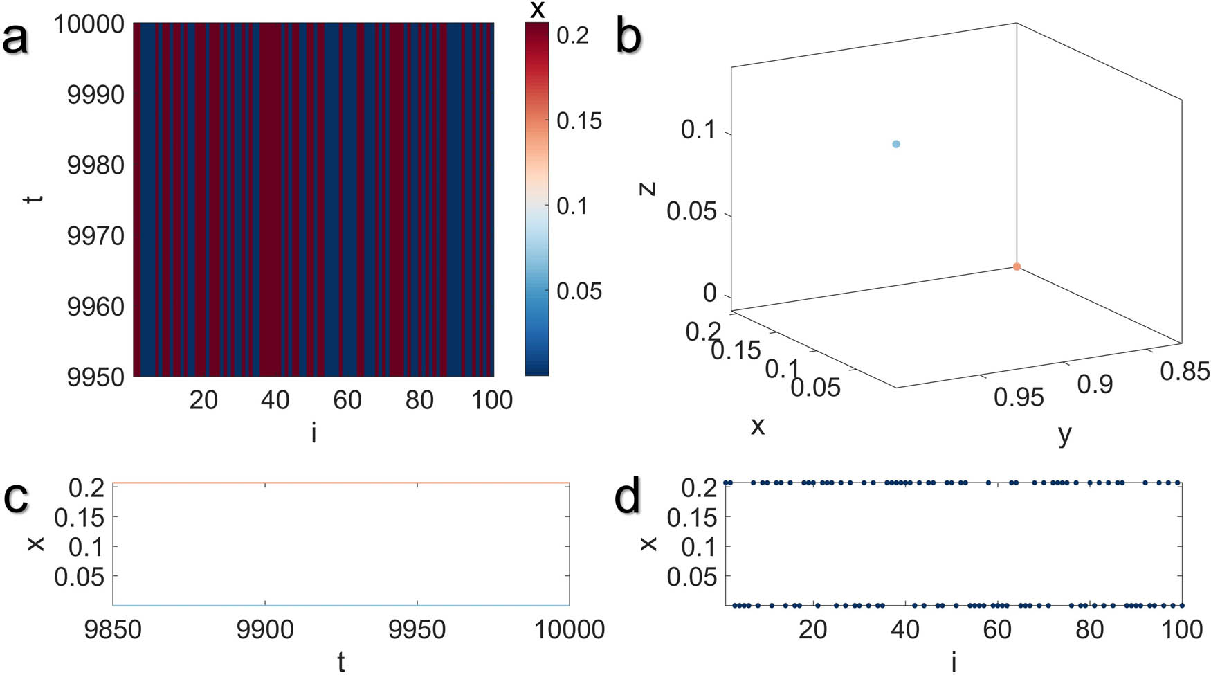
Illustration of the multistable two-cluster synchronization state in the MUL network model with global coupling structure for
We also observe that higher values of
4 Conclusion
In this study, we introduced a network model of MUL systems by incorporating the linear diffusive function of neighboring fast variables into the feedback term. Subsequently, we investigated the synchronization dynamics of this constructed networked model, employing a global coupling scheme. Leveraging the MSF techniques, we provided analytical insights to assess the stability of the synchronization state of the MUL network model. Our results revealed that the coupled MUL models fail to achieve a complete synchronization state, a finding corroborated through numerical analysis by computing the time-averaged synchronization error values. Moving forward, we conducted comprehensive numerical analyses to explore the synchronization patterns within the network. Our findings unveiled that MUL models tend to synchronize into different clusters under varying coupling parameter values. Specifically, in both low and high coupling parameter regimes, the emergence of synchronization clusters was observed. However, under weak connections, two clusters exhibiting homoclinic periodicity coexist, evolving into an anti-phase synchronization state. As connections strengthen, the coexistence of small-amplitude periodic orbits alongside a fixed-point cluster is detected, indicating that some MUL models fail to oscillate and converge to an oscillation death state. With the further strengthening of connections, all MUL models cease oscillating, achieving two distinct synchronous oscillation death states. Despite the increasing proximity of fixed-point solutions, synchronous collapse is never achieved, and the network solution remains almost unchanged until the MUL models become unstable. Conversely, at intermediate coupling strengths, chimera states emerge, accompanied by extreme events observed in MUL model synchronization. Across most observed synchronization patterns, multistability is evident, with solutions demonstrating robustness to variations in the selection of initial conditions around a working point. The results obtained from the coupled MUL network model have practical implications for optimizing synchronization in laser arrays, optical communication systems, and other networked systems. These findings contribute to designing more efficient and stable systems by providing insights into how network size, coupling strength, and structure affect synchronization behavior.
Introducing fractional-order dynamics could allow for a more comprehensive understanding of systems where historical states influence present dynamics [52,53]. Although the current model assumes classical local time derivatives to capture the short-term dynamics of the CO2 laser system, future work could explore the generalization of this model using fractional calculus. Fractional-order derivatives can account for memory effects and nonlocal temporal dependencies, which may enhance the accuracy of the model when long-term or delayed feedback influences are present.
-
Funding information: M.P. was supported by the Slovenian Research and Innovation Agency (Javna agencija za znanstvenoraziskovalno in inovacijsko dejavnost Republike Slovenije) (Grant Nos. P1-0403).
-
Author contributions: MM performed formal analysis and created visualizations. FP conducted the investigation and developed software. KR provided resources and contributed to software development. SJ contributed to the methodology and performed validation. MP was responsible for the conceptualization and validation. RM provided conceptual guidance and supervised the research. All authors contributed to writing and reviewing the manuscript and approved the final version for submission.
-
Conflict of interest: The authors declare that they have no conflict of interest.
-
Data availability statement: Data sharing is not applicable to this article as no new data were created or analyzed in this study.
References
[1] Boccaletti S, Latora V, Moreno Y, Chavez M, Hwang DU. Complex networks: Structure and dynamics. Phys Rep. 2006;424(4):175–308. 10.1016/j.physrep.2005.10.009Suche in Google Scholar
[2] Pecora LM, Carroll TL. Synchronization of chaotic systems. Chaos. 2015;25(9):097611. 10.1063/1.4917383Suche in Google Scholar PubMed
[3] Frasca M, Gambuzza LV, Buscarino A, Fortuna L. Synchronization in networks of nonlinear circuits: Essential topics with MATLABⓇ code. Cham, Switzerland: Springer; 2018. 10.1007/978-3-319-75957-9Suche in Google Scholar
[4] Pecora LM, Sorrentino F, Hagerstrom AM, Murphy TE, Roy R. Cluster synchronization and isolated desynchronization in complex networks with symmetries. Nat Commun. 2014;5(1):4079. 10.1038/ncomms5079Suche in Google Scholar PubMed
[5] Parastesh F, Jafari S, Azarnoush H, Shahriari Z, Wang Z, Boccaletti S, et al. Chimeras. Phys Rep. 2021;898:1–114. 10.1016/j.physrep.2020.10.003Suche in Google Scholar
[6] Wang Z, Hussain I, Pham VT, Kapitaniak T. Discontinuous coupling and transition from synchronization to an intermittent transient chimera state. Sci Iran. 2021;28(Special issue on collective behavior of nonlinear dynamical networks):1661–8. Suche in Google Scholar
[7] Lu L, Ge M, Xu Y, Jia Y. Phase synchronization and mode transition induced by multiple time delays and noises in coupled FitzHugh–Nagumo model. Physica A. 2019;535:122419. 10.1016/j.physa.2019.122419Suche in Google Scholar
[8] Shahverdiev EM, Sivaprakasam S, Shore KA. Lag synchronization in time-delayed systems. Phys Lett A. 2002;292(6):320–4. 10.1016/S0375-9601(01)00824-6Suche in Google Scholar
[9] Rybalova E, Anishchenko VS, Strelkova GI, Zakharova A. Solitary states and solitary state chimera in neural networks. Chaos. 2019;29(7):071106. 10.1063/1.5113789Suche in Google Scholar PubMed
[10] Zheng Z, Huuu G. Generalized synchronization versus phase synchronization. Phys Rev E. 2000;62(6):7882–5. 10.1103/PhysRevE.62.7882Suche in Google Scholar PubMed
[11] Winkler M, Sawicki J, Omelchenko I, Zakharova A, Anishchenko V, Schöll E. Relay synchronization in multiplex networks of discrete maps. Europhys Lett. 2019;126(5):50004. 10.1209/0295-5075/126/50004Suche in Google Scholar
[12] Majhi S, Bera BK, Ghosh D, Perc M. Chimera states in neuronal networks: A review. Phys Life Rev. 2019;28:100–21. 10.1016/j.plrev.2018.09.003Suche in Google Scholar PubMed
[13] Majhi S, Perc M, Ghosh D. Chimera states in a multilayer network of coupled and uncoupled neurons. Chaos. 2017;27(7):073109. 10.1063/1.4993836Suche in Google Scholar PubMed
[14] Hu X, Wu Y, Ding Q, Xie Y, Ye Z, Jia Y. Synchronization of scale-free neuronal network with small-world property induced by spike-timing-dependent plasticity under time delay. Physica D. 2024;460:134091. 10.1016/j.physd.2024.134091Suche in Google Scholar
[15] Mehrabbeik M, Jafari S, Meucci R, Perc M. Synchronization and multistability in a network of diffusively coupled laser models. Commun Nonlinear Sci Numer Simul. 2023;125:107380. 10.1016/j.cnsns.2023.107380Suche in Google Scholar
[16] Olmi S, Gambuzza LV, Frasca M. Multilayer control of synchronization and cascading failures in power grids. Chaos Solit Fractals. 2024;180:114412. 10.1016/j.chaos.2023.114412Suche in Google Scholar
[17] Gambuzza LV, Buscarino A, Chessari S, Fortuna L, Meucci R, Frasca M. Experimental investigation of chimera states with quiescent and synchronous domains in coupled electronic oscillators. Phys Rev E. 2014;90(3):032905. 10.1103/PhysRevE.90.032905Suche in Google Scholar PubMed
[18] Wang Z, Parastesh F, Natiq H, Li J, Xi X, Mehrabbeik M. Synchronization patterns in a network of diffusively delay-coupled memristive Chialvo neuron map. Phys Lett A. 2024;514–515:129607. 10.1016/j.physleta.2024.129607Suche in Google Scholar
[19] Wang Z, Chen M, Xi X, Tian H, Yang R. Multi-chimera states in a higher order network of FitzHugh–Nagumo oscillators. Eur Phys J Spec Top. 2024;233(4):779–86. 10.1140/epjs/s11734-024-01143-0Suche in Google Scholar
[20] Wang Z, Ramamoorthy R, Xi X, Namazi H. Synchronization of the neurons coupled with sequential developing electrical and chemical synapses. Math Biosci Eng. 2022;19(2):1877–90. 10.3934/mbe.2022088Suche in Google Scholar PubMed
[21] Haken H. Analogy between higher instabilities in fluids and lasers. Phys Lett A. 1975;53(1):77–8. 10.1016/0375-9601(75)90353-9Suche in Google Scholar
[22] Agrawal GP. Effect of gain nonlinearities on period doubling and chaos in directly modulated semiconductor lasers. Appl Phys Lett. 1986;49(16):1013–5. 10.1063/1.97456Suche in Google Scholar
[23] Ciofini M, Labate A, Meucci R, Galanti M. Stabilization of unstable fixed points in the dynamics of a laser with feedback. Phys Rev E. 1999;60(1):398–402. 10.1103/PhysRevE.60.398Suche in Google Scholar PubMed
[24] Meucci R, Euzzor S, Tito Arecchi F, Ginoux JM. Minimal universal model for chaos in laser with feedback. Int J Bifurcat Chaos. 2021;31(04):2130013. 10.1142/S0218127421300135Suche in Google Scholar
[25] Meucci R, Marc Ginoux J, Mehrabbeik M, Jafari S, Clinton Sprott J. Generalized multistability and its control in a laser. Chaos. 2022;32(8):083111. 10.1063/5.0093727Suche in Google Scholar PubMed
[26] Uchida A, Rogister F, Garciiia-Ojalvo J, Roy R. Synchronization and communication with chaotic laser systems. vol. 48. Amsterdam, Netherlands: Elsevier; 2005. p. 203–341. 10.1016/S0079-6638(05)48005-1Suche in Google Scholar
[27] Sugawara T, Tachikawa M, Tsukamoto T, Shimizu T. Observation of synchronization in laser chaos. Phys Rev Lett. 1994;72(22):3502–5. 10.1103/PhysRevLett.72.3502Suche in Google Scholar PubMed
[28] Mariño IP, Allaria E, Sanjuán MAF, Meucci R, Arecchi FT. Coupling scheme for complete synchronization of periodically forced chaotic CO2 lasers. Phys Rev E. 2004;70(3):036208. 10.1103/PhysRevE.70.036208Suche in Google Scholar PubMed
[29] DeShazer DJ, Breban R, Ott E, Roy R. Detecting phase synchronization in a chaotic laser array. Phys Rev Lett. 2001;87(4):044101. 10.1103/PhysRevLett.87.044101Suche in Google Scholar PubMed
[30] Hillbrand J, Auth D, Piccardo M, Opačak N, Gornik E, Strasser G, et al. In-phase and anti-phase synchronization in a laser frequency comb. Phys Rev Lett. 2020;124(2):023901. 10.1103/PhysRevLett.124.023901Suche in Google Scholar PubMed
[31] Mihana T, Fujii K, Kanno K, Naruse M, Uchida A. Laser network decision making by lag synchronization of chaos in a ring configuration. Opt Express. 2020;28(26):40112–30. 10.1364/OE.411140Suche in Google Scholar PubMed
[32] Zhang L, Pan W, Yan L, Luo B, Zou X, Xu M. Cluster synchronization of coupled semiconductor lasers network with complex topology. IEEE J Sel Top Quantum Electron. 2019;25(6):1–7. 10.1109/JSTQE.2019.2913010Suche in Google Scholar
[33] Chembo Kouomou Y, Woafo P. Cluster synchronization in coupled chaotic semiconductor lasers and application to switching in chaos-secured communication networks. Opt Commun. 2003;223(4):283–93. 10.1016/S0030-4018(03)01683-3Suche in Google Scholar
[34] Röhm A, Böhm F, Lüdge K. Small chimera states without multistability in a globally delay-coupled network of four lasers. Phys Rev E. 2016;94(4):042204. 10.1103/PhysRevE.94.042204Suche in Google Scholar PubMed
[35] Kazakov D, Opačak N, Pilat F, Wang Y, Belyanin A, Schwarz B, et al. Cluster synchronization in a semiconductor laser. APL Photonics. 2024;9(2):026104. 10.1063/5.0187078Suche in Google Scholar
[36] Roy A, Misra AP, Banerjee S. Synchronization in networks of coupled hyperchaotic CO2 lasers. Phys Scr. 2020;95(4):045225. 10.1088/1402-4896/ab6e4dSuche in Google Scholar
[37] Nag Chowdhury S, Ray A, Dana SK, Ghosh D. Extreme events in dynamical systems and random walkers: A review. Phys Rep. 2022;966:1–52. 10.1016/j.physrep.2022.04.001Suche in Google Scholar
[38] Nag Chowdhury S, Ray A, Mishra A, Ghosh D. Extreme events in globally coupled chaotic maps. J Phys Complex. 2021;2(3):035021. 10.1088/2632-072X/ac221fSuche in Google Scholar
[39] Ray A, Rakshit S, Ghosh D, Dana SK. Intermittent large deviation of chaotic trajectory in Ikeda map: Signature of extreme events. Chaos. 2019;29(4):043131. 10.1063/1.5092741Suche in Google Scholar PubMed
[40] Mishra A, Leo Kingston S, Hens C, Kapitaniak T, Feudel U, Dana SK. Routes to extreme events in dynamical systems: Dynamical and statistical characteristics. Chaos. 2020;30(6):063114. 10.1063/1.5144143Suche in Google Scholar PubMed
[41] Ansmann G, Karnatak R, Lehnertz K, Feudel U. Extreme events in excitable systems and mechanisms of their generation. Phys Rev E. 2013;88(5):052911. 10.1103/PhysRevE.88.052911Suche in Google Scholar PubMed
[42] Mishra A, Saha S, Vigneshwaran M, Pal P, Kapitaniak T, Dana SK. Dragon-king-like extreme events in coupled bursting neurons. Phys Rev E. 2018;97(6):062311. 10.1103/PhysRevE.97.062311Suche in Google Scholar PubMed
[43] Chowdhury SN, Majhi S, Ozer M, Ghosh D, Perc M. Synchronization to extreme events in moving agents. New J Phys. 2019;21(7):073048. 10.1088/1367-2630/ab2a1fSuche in Google Scholar
[44] Bao BC, Li QD, Wang N, Xu Q. Multistability in Chuaas circuit with two stable node-foci. Chaos. 2016;26(4):043111. 10.1063/1.4946813Suche in Google Scholar PubMed
[45] Li X, Xie Y, Ye Z, Huang W, Yang L, Zhan X, et al. Chimera-like state in the bistable excitatory-inhibitory cortical neuronal network. Chaos Solit Fractals. 2024;180:114549. 10.1016/j.chaos.2024.114549Suche in Google Scholar
[46] Mehrabbeik M, Jafari S, Ginoux JM, Meucci R. Multistability and its dependence on the attractor volume. Phys Lett A. 2023;485:129088. 10.1016/j.physleta.2023.129088Suche in Google Scholar
[47] Bao BC, Xu Q, Bao H, Chen M. Extreme multistability in a memristive circuit. Electron Lett. 2016;52(12):1008–10. 10.1049/el.2016.0563Suche in Google Scholar
[48] Bao BC, Bao H, Wang N, Chen M, Xu Q. Hidden extreme multistability in memristive hyperchaotic system. Chaos Solit Fractals. 2017;94:102–11. 10.1016/j.chaos.2016.11.016Suche in Google Scholar
[49] Sprott JC, Jafari S, Khalaf AJM, Kapitaniak T. Megastability: Coexistence of a countable infinity of nested attractors in a periodically-forced oscillator with spatially-periodic damping. Eur Phys J Spec Top. 2017;226(9):1979–85. 10.1140/epjst/e2017-70037-1Suche in Google Scholar
[50] Leutcho GD, Khalaf AJM, Njitacke Tabekoueng Z, Fozin TF, Kengne J, Jafari S, et al. A new oscillator with mega-stability and its Hamilton energy: Infinite coexisting hidden and self-excited attractors. Chaos. 2020;30(3):033112. 10.1063/1.5142777Suche in Google Scholar PubMed
[51] Pecora LM, Carroll TL. Master Stability Functions for Synchronized Coupled Systems. Phys Rev Lett. 1998;80(10):2109–12. 10.1103/PhysRevLett.80.2109Suche in Google Scholar
[52] Zhou Y, Zhang Y. Noether symmetries for fractional generalized Birkhoffian systems in terms of classical and combined Caputo derivatives. Acta Mech. 2020;231(7):3017–29. 10.1007/s00707-020-02690-ySuche in Google Scholar
[53] Sumelka W, Łuczak B, Gajewski T, Voyiadjis GZ. Modelling of AAA in the framework of time-fractional damage hyperelasticity. Int J Solids Struct. 2020;206:30–42. 10.1016/j.ijsolstr.2020.08.015Suche in Google Scholar
© 2024 the author(s), published by De Gruyter
This work is licensed under the Creative Commons Attribution 4.0 International License.
Artikel in diesem Heft
- Editorial
- Focus on NLENG 2023 Volume 12 Issue 1
- Research Articles
- Seismic vulnerability signal analysis of low tower cable-stayed bridges method based on convolutional attention network
- Robust passivity-based nonlinear controller design for bilateral teleoperation system under variable time delay and variable load disturbance
- A physically consistent AI-based SPH emulator for computational fluid dynamics
- Asymmetrical novel hyperchaotic system with two exponential functions and an application to image encryption
- A novel framework for effective structural vulnerability assessment of tubular structures using machine learning algorithms (GA and ANN) for hybrid simulations
- Flow and irreversible mechanism of pure and hybridized non-Newtonian nanofluids through elastic surfaces with melting effects
- Stability analysis of the corruption dynamics under fractional-order interventions
- Solutions of certain initial-boundary value problems via a new extended Laplace transform
- Numerical solution of two-dimensional fractional differential equations using Laplace transform with residual power series method
- Fractional-order lead networks to avoid limit cycle in control loops with dead zone and plant servo system
- Modeling anomalous transport in fractal porous media: A study of fractional diffusion PDEs using numerical method
- Analysis of nonlinear dynamics of RC slabs under blast loads: A hybrid machine learning approach
- On theoretical and numerical analysis of fractal--fractional non-linear hybrid differential equations
- Traveling wave solutions, numerical solutions, and stability analysis of the (2+1) conformal time-fractional generalized q-deformed sinh-Gordon equation
- Influence of damage on large displacement buckling analysis of beams
- Approximate numerical procedures for the Navier–Stokes system through the generalized method of lines
- Mathematical analysis of a combustible viscoelastic material in a cylindrical channel taking into account induced electric field: A spectral approach
- A new operational matrix method to solve nonlinear fractional differential equations
- New solutions for the generalized q-deformed wave equation with q-translation symmetry
- Optimize the corrosion behaviour and mechanical properties of AISI 316 stainless steel under heat treatment and previous cold working
- Soliton dynamics of the KdV–mKdV equation using three distinct exact methods in nonlinear phenomena
- Investigation of the lubrication performance of a marine diesel engine crankshaft using a thermo-electrohydrodynamic model
- Modeling credit risk with mixed fractional Brownian motion: An application to barrier options
- Method of feature extraction of abnormal communication signal in network based on nonlinear technology
- An innovative binocular vision-based method for displacement measurement in membrane structures
- An analysis of exponential kernel fractional difference operator for delta positivity
- Novel analytic solutions of strain wave model in micro-structured solids
- Conditions for the existence of soliton solutions: An analysis of coefficients in the generalized Wu–Zhang system and generalized Sawada–Kotera model
- Scale-3 Haar wavelet-based method of fractal-fractional differential equations with power law kernel and exponential decay kernel
- Non-linear influences of track dynamic irregularities on vertical levelling loss of heavy-haul railway track geometry under cyclic loadings
- Fast analysis approach for instability problems of thin shells utilizing ANNs and a Bayesian regularization back-propagation algorithm
- Validity and error analysis of calculating matrix exponential function and vector product
- Optimizing execution time and cost while scheduling scientific workflow in edge data center with fault tolerance awareness
- Estimating the dynamics of the drinking epidemic model with control interventions: A sensitivity analysis
- Online and offline physical education quality assessment based on mobile edge computing
- Discovering optical solutions to a nonlinear Schrödinger equation and its bifurcation and chaos analysis
- New convolved Fibonacci collocation procedure for the Fitzhugh–Nagumo non-linear equation
- Study of weakly nonlinear double-diffusive magneto-convection with throughflow under concentration modulation
- Variable sampling time discrete sliding mode control for a flapping wing micro air vehicle using flapping frequency as the control input
- Error analysis of arbitrarily high-order stepping schemes for fractional integro-differential equations with weakly singular kernels
- Solitary and periodic pattern solutions for time-fractional generalized nonlinear Schrödinger equation
- An unconditionally stable numerical scheme for solving nonlinear Fisher equation
- Effect of modulated boundary on heat and mass transport of Walter-B viscoelastic fluid saturated in porous medium
- Analysis of heat mass transfer in a squeezed Carreau nanofluid flow due to a sensor surface with variable thermal conductivity
- Navigating waves: Advancing ocean dynamics through the nonlinear Schrödinger equation
- Experimental and numerical investigations into torsional-flexural behaviours of railway composite sleepers and bearers
- Novel dynamics of the fractional KFG equation through the unified and unified solver schemes with stability and multistability analysis
- Analysis of the magnetohydrodynamic effects on non-Newtonian fluid flow in an inclined non-uniform channel under long-wavelength, low-Reynolds number conditions
- Convergence analysis of non-matching finite elements for a linear monotone additive Schwarz scheme for semi-linear elliptic problems
- Global well-posedness and exponential decay estimates for semilinear Newell–Whitehead–Segel equation
- Petrov-Galerkin method for small deflections in fourth-order beam equations in civil engineering
- Solution of third-order nonlinear integro-differential equations with parallel computing for intelligent IoT and wireless networks using the Haar wavelet method
- Mathematical modeling and computational analysis of hepatitis B virus transmission using the higher-order Galerkin scheme
- Mathematical model based on nonlinear differential equations and its control algorithm
- Bifurcation and chaos: Unraveling soliton solutions in a couple fractional-order nonlinear evolution equation
- Space–time variable-order carbon nanotube model using modified Atangana–Baleanu–Caputo derivative
- Minimal universal laser network model: Synchronization, extreme events, and multistability
- Valuation of forward start option with mean reverting stock model for uncertain markets
- Geometric nonlinear analysis based on the generalized displacement control method and orthogonal iteration
- Fuzzy neural network with backpropagation for fuzzy quadratic programming problems and portfolio optimization problems
- B-spline curve theory: An overview and applications in real life
- Nonlinearity modeling for online estimation of industrial cooling fan speed subject to model uncertainties and state-dependent measurement noise
- Quantitative analysis and modeling of ride sharing behavior based on internet of vehicles
- Review Article
- Bond performance of recycled coarse aggregate concrete with rebar under freeze–thaw environment: A review
- Retraction
- Retraction of “Convolutional neural network for UAV image processing and navigation in tree plantations based on deep learning”
- Special Issue: Dynamic Engineering and Control Methods for the Nonlinear Systems - Part II
- Improved nonlinear model predictive control with inequality constraints using particle filtering for nonlinear and highly coupled dynamical systems
- Anti-control of Hopf bifurcation for a chaotic system
- Special Issue: Decision and Control in Nonlinear Systems - Part I
- Addressing target loss and actuator saturation in visual servoing of multirotors: A nonrecursive augmented dynamics control approach
- Collaborative control of multi-manipulator systems in intelligent manufacturing based on event-triggered and adaptive strategy
- Greenhouse monitoring system integrating NB-IOT technology and a cloud service framework
- Special Issue: Unleashing the Power of AI and ML in Dynamical System Research
- Computational analysis of the Covid-19 model using the continuous Galerkin–Petrov scheme
- Special Issue: Nonlinear Analysis and Design of Communication Networks for IoT Applications - Part I
- Research on the role of multi-sensor system information fusion in improving hardware control accuracy of intelligent system
- Advanced integration of IoT and AI algorithms for comprehensive smart meter data analysis in smart grids