Approximate numerical procedures for the Navier–Stokes system through the generalized method of lines
-
Fabio Silva Botelho


Abstract
This article develops approximate numerical solutions through the generalized method of lines for the time-independent, incompressible Navier–Stokes system in fluid mechanics. More specifically, we highlight the main objective of this article is the development of new approximate procedures for solving numerically the equation systems originated from a domain discretization related to a finite differences scheme. We recall that for such a method, the domain of the partial differential equation in question is discretized in lines (or more generally in curves), and the concerning solutions are written on these lines as functions of the boundary conditions and the domain boundary shape. Finally, it is worth emphasizing that in this text, we have presented softwares and results for a concerning approximate proximal approach, as well as results based on the original conception of the generalized method of lines.
1 Introduction
In this article, we develop approximate solutions for the time-independent incompressible Navier–Stokes system through the generalized method of lines. We recall again that, for such a method, the domain of the partial differential equation in question is discretized in lines and the concerning solution is written on these lines as functions of the boundary conditions and the domain boundary shape. It is worth highlighting that the main aim of this article is the development of a new approximate procedure for solving numerically the equation system originated from a domain discretization concerning standard finite difference schemes to be specified for each case addressed. We also emphasize the first article part concerns the application and extension of an approximate proximal approach published in the study by Botelho [1]. We develop an analogous algorithm as those presented by Botelho [1] but now for a Navier–Stokes system, which is more complex than the systems of partial differential equations previously addressed. In this first step, we present an algorithm and respective software in MAT-LAB.
Furthermore, we have developed and presented related softwares in MATHEMATICA for a simpler type of domain and also concerning the mentioned proximal approach. Finally, in the last section, we present a software and related line expressions through the original conception of the generalized method of lines, so that in such related numerical examples, the main results are established through applications of the Banach fixed point theorem.
Remark 1.1
We also highlight that the next two paragraphs in this article (a relatively small part) overlap with the Chapter 28, starting page 526, in the book by Botelho, [2], published in 2020, by CRC Taylor and Francis. However, we emphasize that the present article includes substantial new parts, including a concerning software not included in the previous version of 2020. Another novelty in the present version is the establishment of appropriate boundary conditions for an equivalent elliptic system to the original Navier–Stokes one. Such new boundary conditions and concerning results are indicated in Section 2.
At this point, we describe the system in question.
Consider
Under such notation and statements, the time-independent incompressible Navier–Stokes system of partial differential equations stands for
At first, we look for solutions
About the references, we emphasize that related existence of numerical and theoretical results for similar systems may be found in [4–9] and [10], respectively. In particular Temam [10] addresses extensively both theoretical and numerical methods and an interesting interplay between them. Moreover, related finite difference schemes are addressed in the study by Strikwerda [11].
Finally, it is worth mentioning that this article has been published as a preprint (see the concerning reference [12] for details).
2 Details about an equivalent elliptic system
Defining now
As previously mentioned, at first, we look for solutions
We are going to obtain an equivalent elliptic system with appropriate boundary conditions.
Our main result is summarized by the following theorem.
Theorem 2.1
Let
Assume
Suppose also, for such u, v fixed, the unique solution of equation in
with the boundary conditions
is
Under such hypotheses,
Proof
In Eq. (5), taking the derivative in
From the hypotheses,
From this and Eq. (9), we obtain
Denoting
From the hypotheses, the unique solution of this last equation with the boundary conditions
From this and Eq. (10), we have
in
The proof is complete.
Remark 2.2
The process of obtaining such a system with a Laplace operator in
The novelty here is the identification of the correct related boundary conditions obtained through an appropriate solution of Eq. (10).
3 An approximate proximal approach
In this section, we develop an approximate proximal numerical procedure for the model in question.
Such results are extensions of previous ones published in the study by Botelho [1], now for the Navier–Stokes system context.
More specifically, neglecting the gravity field, we solve the following system of equations:
We present a software similar to those presented in the study by Botelho [1], with
and with the boundary conditions
Eq. (11), in an appropriate partial finite difference scheme, stands for
After linearizing such a system about
At this point, denoting
and
Therefore, we may write
where
In particular, for
so that
where
Similarly, for
so that
where
Reasoning inductively, having
we obtain
where
Observe now that
This last equation is a second-order ODE in
Summarizing, we have obtained
Similarly, we may obtain
Having
Similarly, we may obtain
Having
Similarly, we may obtain
And so on, up to obtaining
The next step is to replace
Here, we present a concerning software in MAT-LAB based in this last algorithm (with small changes and differences where we have set
*******************************
clear all
m8=500;
d=1/m8;
m9=140;
d1=1/m9;
e1=0.01;
K=155.0;
m2=zeros(m9-1,m9-1);
for i=2:m9-2
m2(i,i)=-2.0;
m2(i,i+1)=1.0;
m2(i,i-1)=1.0;
end;
m2(1,1)=-1.0;
m2(1,2)=1.0;
m2(m9-1,m9-1)=-1.0;
m2(m9-1,m9-2)=1.0;
m22=zeros(m9-1,m9-1);
for i=2:m9-2
m22(i,i)=-2.0;
m22(i,i+1)=1.0;
m22(i,i-1)=1.0;
end;
m22(1,1)=-2.0;
m22(1,2)=1.0;
m22(m9-1,m9-1)=-2.0;
m22(m9-1,m9-2)=1.0;
m1a=zeros(m9-1,m9-1);
m1b=zeros(m9-1,m9-1);
for i=1:m9-2
m1a(i,i)=-1.0;
m1a(i,i+1)=1.0;
end;
m1a(m9-1,m9-1)=-1.0;
for i=2:m9-1
m1b(i,i)=1.0;
m1b(i,i-1)=-1.0;
end;
m1b(1,1)=1.0;
m1=(m1a+m1b)/2;
Id=eye(m9-1);
a(1)=1/(2+K*
b(1)=1/(2+K*
c(1)=1/(2+K*
for i=2:m8-1
a(i)=1/(2-a(i-1)+K*
b(i)=a(i)*b(i-1);
c(i)=(c(i-1)+1)*a(i);
end;
for i=1:m9-1
u5(i,1)=0.55*i*d1*(1-i*d1);
end;
uo=u5;
o=zeros(m9-1,1);
po=0.15*ones(m9-1,1);
for i=1:m8-1
Uo(:,i)=0.25*ones(m9-1,1);
Vo(:,i)=0.05*ones(m9-1,1);
Po(:,i)=0.05*ones(m9-1,1);
end;
for i=1:m8-1
U1(:,i)=Uo(:,i);
V1(:,i)=Vo(:,i);
P1(:,i)=Po(:,i);
end;
for k7=1:1
e1=e1*.94;
b14=1.0;
k1=1;
k1max=3000;
while
k1=k1+1;
a(1)=1/(2+K*
b(1)=a(1);
c1(:,1)=a(1)*K*Uo(:,1)*
c2(:,1)=a(1)*K*Vo(:,1)*
c3(:,1)=a(1)*(K*Po(:,1)*
for i=2:m8-1
a(i)=1/(2+K*
b(i)=a(i)*(b(i-1));
c1(:,i)=a(i)*(c1(:,i-1)+K*Uo(:,i)*
c2(:,i)=a(i)*(c2(:,i-1)+K*Vo(:,i)*
c3(:,i)=a(i)*(c3(:,i-1)+K*Po(:,i)*
end;
i=1;
M50=(Id-a(m8-1)*Id-c(m8-1)*m22/
z1=b(m8-1)*uo+c1(:,m8-i)+c(m8-1)*(-Vo(:,m8-i).*(m1*Uo(:,m8-i)))/d1*
M60=(Id-a(m8-1)*Id-c(m8-1)*m22/
z2=b(m8-1)*vo+c2(:,m8-i)+c(m8-1)*(-Vo(:,m8-i)).*(m1*Vo(:,m8-i))/d1*
M70=(Id-a(m8-1)*Id-c(m8-1)*m2/
z3=b(m8-1)*po+c(m8-1)*((m1/d1*Vo(:,m8-i)).*(m1/d1*Vo(:,m8-i))*
U(:,m8-1)=inv(M50)*z1;
V(:,m8-1)=inv(M60)*z2;
P(:,m8-1)=inv(M70)*z3;
for i=2:m8-1
M50=(Id-c(m8-i)*m22/
z1=b(m8-i)*uo+a(m8-i)*U(:,m8-i+1);
z1=z1+c(m8-i)*(-U(:,m8-i+1).*(Uo(:,m8-i+1)-Uo(:,m8-i))*d/e1;
z1=z1-(Po(:,m8-i+1)-Po(:,m8-i))*d/e1);
z1=z1+c1(:,m8-i);
z1=z1+c(m8-i)*(-V(:,m8-i+1).*(m1*Uo(:,m8-i))/d1*
M60=(Id-c(m8-i)*m22/
z2=b(m8-i)*vo+a(m8-i)*V(:,m8-i+1);
z2=z2+c(m8-i)*(-(U(:,m8-i+1).*(Vo(:,m8-i+1)-Vo(:,m8-i))*d/e1;
z2=z2+V(:,m8-i+1)).*(m1*Vo(:,m8-i)/d1*
z2=z2-c(m8-i)*(m1*Po(:,m8-i)/d1*
z2=z2+c2(:,m8-i);
M70=(Id-c(m8-i)*m2/
z3=b(m8-i)*po+a(m8-i)*P(:,m8-i+1);
z3=z3+c(m8-i)*((Uo(:,m8-i+1)-Uo(:,m8-i)).*(Uo(:,m8-i+1)-Uo(:,m8-i));
z3=z3+(m1/d1*Vo(:,m8-i)).*(m1/d1*Vo(:,m8-i))*
z3=z3+2*(m1/d1*Uo(:,m8-i)).*(Vo(:,m8-i+1)-Vo(:,m8-i))*d;
z3=z3+c3(:,m8-i);
U(:,m8-i)=inv(M50)*z1;
V(:,m8-i)=inv(M60)*z2;
P(:,m8-i)=inv(M70)*z3;
end;
b14=max(max(abs(U-Uo)));
b14
Uo=U;
Vo=V;
Po=P;
k1
U(m9/2,10)
end;
k7
end;
for i=1:m9-1
y(i)=i*d1;
end;
for i=1:m8-1
x(i)=i*d;
end;
mesh(x,y,U);
**********************************
For the field of velocities
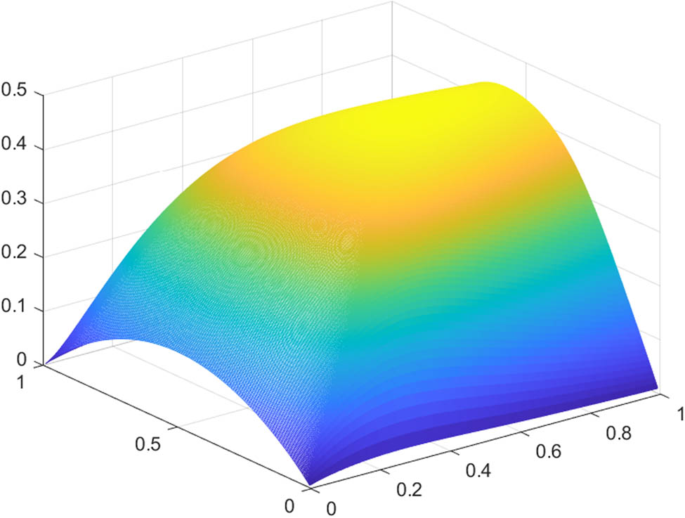
Solution
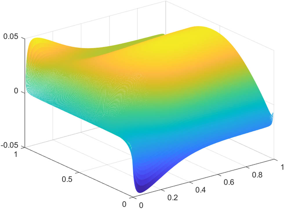
Solution

Solution
4 A software in MATHEMATICA related to the previous algorithm
In this section, we develop the solution for the Navier–Stokes system through the generalized method of lines, similar to the results presented in the study by Botelho [1], but now in a Navier–Stokes system context.
We present a software in MATHEMATICA for
We consider it in polar coordinates, with
and
The boundary conditions are
From now and on,
We remark that some changes have been made, concerning the original conception, in order to make it suitable through the software MATHEMATICA for such a Navier–Stokes system.
We highlight that the approximation error for the computation between two adjacent lines is proportional to
At this point, we provide some details about the numerical procedure.
For
where
Thus, the concerning approximate Navier–Stokes system stands for
Similarly as in the previous section, we may obtain
where the process to obtain
Observe that for
and
Similarly, we may obtain
and so on up to obtaining
The next step is to replace
by
and then to repeat the process until an appropriate convergence criterion is satisfied.
Here the concerning software.
*************************************************
Here we present the related line expressions obtained for the lines
1.
2.
3.
5 The software and numerical results for a more specific example
In this section, we present numerical results for the same Navier–Stokes system and domain as in the previous one, but now with different boundary conditions.
In this example, we set
Here the concerning software:
*************************************************
1.
2.
3.
4.
5.
6.
7.
8.
9.
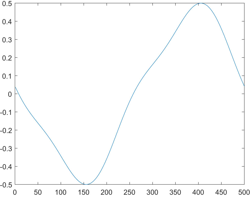
Here, we present the related plots for the lines
For each line, we set
For such lines, please see Figures 4, 5, 6, and 7, respectively.

Solution
Solution
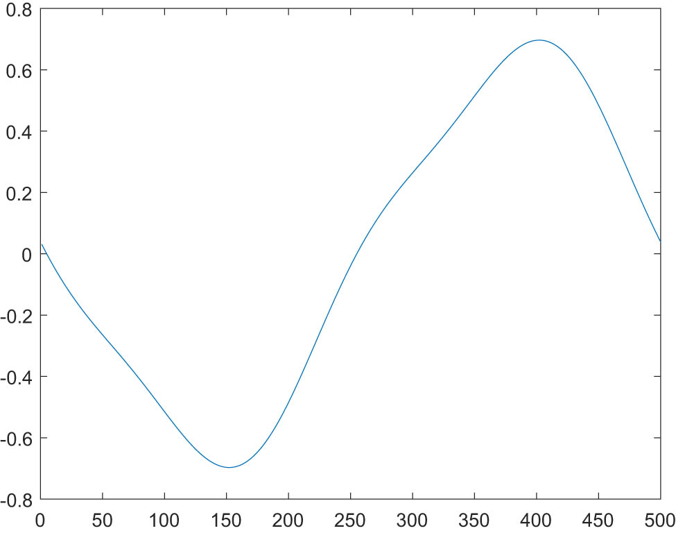
Solution
Solution
6 Numerical results through the original conception of the generalized method of lines for the Navier–Stokes system
In this section, we develop the solution for the Navier–Stokes system through the generalized method of lines, as originally introduced in [13], with further developments in [14].
We present a software in MATHEMATICA for
Such a software refers to an algorithm presented in Chapter 27, in [2], in polar coordinates, with
and
The boundary conditions are
We remark some changes have been made, concerning the original conception, to make it suitable through the software MATHEMATICA for such a Navier–Stokes system.
We highlight that the nature of this approximation is qualitative.
Here the concerning software in MATHEMATICA.
****************************************
***************************************************
Here, the line expressions for the field of velocity
1.
2.
3.
4.
5.
6.
7.
8.
9.
7 Conclusion
In this article, we have presented solutions for examples concerning the two-dimensional, time-independent, and incompressible Navier–Stokes system through the generalized method of lines. In particular, we have developed software in MAT-LAB and MATHEMATICA for approximate solutions of the numerical systems originated from a full (for the MAT-LAB software) and partial (for the MATHEMATICA codes) domain discretization concerning appropriate finite difference schemes. It is worth highlighting that, with little adaptations, it is possible to apply the MAT-LAB software for a very large class of domain shapes and related boundary conditions. We also obtain the appropriate boundary conditions for an equivalent elliptic system to the original Navier–Stokes one.
Finally, the extension of such results to
-
Funding information: The author states that there is no external funding involved.
-
Author contributions: The author has the entire responsibility for the entire content of this manuscript and approved its submission.
-
Conflict of interest: The author declares no conflict of interest concerning this article.
-
Data availability statement: Details on the software for numerical results available upon request.
References
[1] Botelho FS. An approximate proximal numerical procedure concerning the generalized method of lines. Mathematics 2022;10(16):2950. 10.3390/math10162950. Suche in Google Scholar
[2] Botelho FS. Functional analysis, calculus of variations and numerical methods in physics and engineering. Boca Raton (FL), USA: Taylor and Francis; 2020. 10.1201/9780429343315Suche in Google Scholar
[3] Adams RA, Fournier JF. Sobolev spaces. 2nd ed. New York (NY), USA: Elsevier; 2003. Suche in Google Scholar
[4] Constantin P, Foias C. Navier-Stokes equation. Chicago (IL), USA: University of Chicago Press; 1989. 10.7208/chicago/9780226764320.001.0001Suche in Google Scholar
[5] Hamouda M, Han D, Jung C-Y, Temam R. Boundary layers for the 3D primitive equations in a cube: the zero-mode. J Appl Anal Comput. 2018;8(3):873–89. 10.11948/2018.873. Suche in Google Scholar
[6] Giorgini A, Miranville A, Temam R. Uniqueness and regularity for the Navier-Stokes-Cahn-Hilliard system. SIAM J Math Anal (SIMA). 2019;51(3):2535–74. 10.1137/18M1223459. Suche in Google Scholar
[7] Foias C, Rosa RM, Temam R. Properties of stationary statistical solutions of the three-dimensional Navier-Stokes equations. J Dyn Differ Equ Special Issue in Memory of George Sell. 2019;31(3):1689–741. 10.1007/s10884-018-9719-2. Suche in Google Scholar
[8] Ben Omrane I, Ben Slimane M, Gala S, Ragusa MA. Regularity results for solutions of micropolar fluid equations in terms of the pressure. AIMS Math. 2023;8(9):21208–20. 10.3934/math.20231081. Suche in Google Scholar
[9] Alharbi FM, Naeem M, Zubair M, Jawad M, Jan WU, Jan R. Bioconvection due to gyrotactic microorganisms in couple stress hybrid nanofluid laminar mixed convection incompressible flow with magnetic nanoparticles and chemical reaction as carrier for targeted drug delivery through porous stretching sheet. Molecules 2021;26(13):3954. 10.3390/molecules26133954Suche in Google Scholar PubMed PubMed Central
[10] Temam R. Navier-Stokes equations. AMS Chelsea, reprint 2001. 10.1090/chel/343Suche in Google Scholar
[11] Strikwerda JC. Finite difference schemes and partial differential equations. 2nd ed. Philadelphia (PA), USA: SIAM; 2004. 10.1137/1.9780898717938Suche in Google Scholar
[12] Botelho FS. Approximate numerical procedures for the Navier-Stokes system through the generalized method of lines. Preprints.org 2023. id: 2023020422. https://doi.org/10.20944/preprints202302.0422.v3. Suche in Google Scholar
[13] Botelho F. Topics on functional analysis, calculus of variations and duality. Sofia, Bulgaria: Academic Publications; 2011. Suche in Google Scholar
[14] Botelho F. Existence of solution for the Ginzburg-Landau system, a related optimal control problem and its computation by the generalized method of lines. Appl Math Comput. 2012;218:11976–89. 10.1016/j.amc.2012.05.067Suche in Google Scholar
© 2024 the author(s), published by De Gruyter
This work is licensed under the Creative Commons Attribution 4.0 International License.
Artikel in diesem Heft
- Editorial
- Focus on NLENG 2023 Volume 12 Issue 1
- Research Articles
- Seismic vulnerability signal analysis of low tower cable-stayed bridges method based on convolutional attention network
- Robust passivity-based nonlinear controller design for bilateral teleoperation system under variable time delay and variable load disturbance
- A physically consistent AI-based SPH emulator for computational fluid dynamics
- Asymmetrical novel hyperchaotic system with two exponential functions and an application to image encryption
- A novel framework for effective structural vulnerability assessment of tubular structures using machine learning algorithms (GA and ANN) for hybrid simulations
- Flow and irreversible mechanism of pure and hybridized non-Newtonian nanofluids through elastic surfaces with melting effects
- Stability analysis of the corruption dynamics under fractional-order interventions
- Solutions of certain initial-boundary value problems via a new extended Laplace transform
- Numerical solution of two-dimensional fractional differential equations using Laplace transform with residual power series method
- Fractional-order lead networks to avoid limit cycle in control loops with dead zone and plant servo system
- Modeling anomalous transport in fractal porous media: A study of fractional diffusion PDEs using numerical method
- Analysis of nonlinear dynamics of RC slabs under blast loads: A hybrid machine learning approach
- On theoretical and numerical analysis of fractal--fractional non-linear hybrid differential equations
- Traveling wave solutions, numerical solutions, and stability analysis of the (2+1) conformal time-fractional generalized q-deformed sinh-Gordon equation
- Influence of damage on large displacement buckling analysis of beams
- Approximate numerical procedures for the Navier–Stokes system through the generalized method of lines
- Mathematical analysis of a combustible viscoelastic material in a cylindrical channel taking into account induced electric field: A spectral approach
- A new operational matrix method to solve nonlinear fractional differential equations
- New solutions for the generalized q-deformed wave equation with q-translation symmetry
- Optimize the corrosion behaviour and mechanical properties of AISI 316 stainless steel under heat treatment and previous cold working
- Soliton dynamics of the KdV–mKdV equation using three distinct exact methods in nonlinear phenomena
- Investigation of the lubrication performance of a marine diesel engine crankshaft using a thermo-electrohydrodynamic model
- Modeling credit risk with mixed fractional Brownian motion: An application to barrier options
- Method of feature extraction of abnormal communication signal in network based on nonlinear technology
- An innovative binocular vision-based method for displacement measurement in membrane structures
- An analysis of exponential kernel fractional difference operator for delta positivity
- Novel analytic solutions of strain wave model in micro-structured solids
- Conditions for the existence of soliton solutions: An analysis of coefficients in the generalized Wu–Zhang system and generalized Sawada–Kotera model
- Scale-3 Haar wavelet-based method of fractal-fractional differential equations with power law kernel and exponential decay kernel
- Non-linear influences of track dynamic irregularities on vertical levelling loss of heavy-haul railway track geometry under cyclic loadings
- Fast analysis approach for instability problems of thin shells utilizing ANNs and a Bayesian regularization back-propagation algorithm
- Validity and error analysis of calculating matrix exponential function and vector product
- Optimizing execution time and cost while scheduling scientific workflow in edge data center with fault tolerance awareness
- Estimating the dynamics of the drinking epidemic model with control interventions: A sensitivity analysis
- Online and offline physical education quality assessment based on mobile edge computing
- Discovering optical solutions to a nonlinear Schrödinger equation and its bifurcation and chaos analysis
- New convolved Fibonacci collocation procedure for the Fitzhugh–Nagumo non-linear equation
- Study of weakly nonlinear double-diffusive magneto-convection with throughflow under concentration modulation
- Variable sampling time discrete sliding mode control for a flapping wing micro air vehicle using flapping frequency as the control input
- Error analysis of arbitrarily high-order stepping schemes for fractional integro-differential equations with weakly singular kernels
- Solitary and periodic pattern solutions for time-fractional generalized nonlinear Schrödinger equation
- An unconditionally stable numerical scheme for solving nonlinear Fisher equation
- Effect of modulated boundary on heat and mass transport of Walter-B viscoelastic fluid saturated in porous medium
- Analysis of heat mass transfer in a squeezed Carreau nanofluid flow due to a sensor surface with variable thermal conductivity
- Navigating waves: Advancing ocean dynamics through the nonlinear Schrödinger equation
- Experimental and numerical investigations into torsional-flexural behaviours of railway composite sleepers and bearers
- Novel dynamics of the fractional KFG equation through the unified and unified solver schemes with stability and multistability analysis
- Analysis of the magnetohydrodynamic effects on non-Newtonian fluid flow in an inclined non-uniform channel under long-wavelength, low-Reynolds number conditions
- Convergence analysis of non-matching finite elements for a linear monotone additive Schwarz scheme for semi-linear elliptic problems
- Global well-posedness and exponential decay estimates for semilinear Newell–Whitehead–Segel equation
- Petrov-Galerkin method for small deflections in fourth-order beam equations in civil engineering
- Solution of third-order nonlinear integro-differential equations with parallel computing for intelligent IoT and wireless networks using the Haar wavelet method
- Mathematical modeling and computational analysis of hepatitis B virus transmission using the higher-order Galerkin scheme
- Mathematical model based on nonlinear differential equations and its control algorithm
- Bifurcation and chaos: Unraveling soliton solutions in a couple fractional-order nonlinear evolution equation
- Space–time variable-order carbon nanotube model using modified Atangana–Baleanu–Caputo derivative
- Minimal universal laser network model: Synchronization, extreme events, and multistability
- Valuation of forward start option with mean reverting stock model for uncertain markets
- Geometric nonlinear analysis based on the generalized displacement control method and orthogonal iteration
- Fuzzy neural network with backpropagation for fuzzy quadratic programming problems and portfolio optimization problems
- B-spline curve theory: An overview and applications in real life
- Nonlinearity modeling for online estimation of industrial cooling fan speed subject to model uncertainties and state-dependent measurement noise
- Quantitative analysis and modeling of ride sharing behavior based on internet of vehicles
- Review Article
- Bond performance of recycled coarse aggregate concrete with rebar under freeze–thaw environment: A review
- Retraction
- Retraction of “Convolutional neural network for UAV image processing and navigation in tree plantations based on deep learning”
- Special Issue: Dynamic Engineering and Control Methods for the Nonlinear Systems - Part II
- Improved nonlinear model predictive control with inequality constraints using particle filtering for nonlinear and highly coupled dynamical systems
- Anti-control of Hopf bifurcation for a chaotic system
- Special Issue: Decision and Control in Nonlinear Systems - Part I
- Addressing target loss and actuator saturation in visual servoing of multirotors: A nonrecursive augmented dynamics control approach
- Collaborative control of multi-manipulator systems in intelligent manufacturing based on event-triggered and adaptive strategy
- Greenhouse monitoring system integrating NB-IOT technology and a cloud service framework
- Special Issue: Unleashing the Power of AI and ML in Dynamical System Research
- Computational analysis of the Covid-19 model using the continuous Galerkin–Petrov scheme
- Special Issue: Nonlinear Analysis and Design of Communication Networks for IoT Applications - Part I
- Research on the role of multi-sensor system information fusion in improving hardware control accuracy of intelligent system
- Advanced integration of IoT and AI algorithms for comprehensive smart meter data analysis in smart grids