Numerical analysis of thermophoretic particle deposition on 3D Casson nanofluid: Artificial neural networks-based Levenberg–Marquardt algorithm

Amna Khan; Fahad Aljuaydi; Zeeshan Khan; Saeed Islam

doi:10.1515/phys-2023-0181

Article Open Access

Numerical analysis of thermophoretic particle deposition on 3D Casson nanofluid: Artificial neural networks-based Levenberg–Marquardt algorithm

Amna Khan , Fahad Aljuaydi , Zeeshan Khan and Saeed Islam

Published/Copyright: February 23, 2024

Published by

Become an author with De Gruyter Brill

Submit Manuscript Author Information Explore this Subject

From the journal Open Physics Volume 22 Issue 1

Abstract

The aim of this research is to provide a new computer-assisted approach for predicting thermophoresis particle decomposition on three-dimensional Casson nanofluid flow that passed over a stretched surface (thermophoresis particle decomposition on three-dimensional Casson nanofluid flow; TPD-CNF). In order to understand the flow behavior of nanofluid flow model, an optimized Levenberg–Marquardt learning algorithm with backpropagation neural network (LMLA-BPNN) has been designed. The mathematical model of TPD-CNF framed with appropriate assumptions and turned into ordinary differential equations via suitable similarity transformations are used. The bvp4c approach is used to collect the data for the LMLA-BPNN, which is used for parameters related with the TPD-CNF model controlling the velocity, temperature, and nanofluid concentration profiles. The proposed algorithm LMLA-BPNN is used to evaluate the obtained TDP-CNF model performance in various instances, and a correlation of the findings with a reference dataset is performed to check the validity and efficacy of the proposed algorithm for the analysis of nanofluids flow composed of sodium alginate nanoparticles dispersed in base fluid water. Statistical tools such as Mean square error, State transition dynamics, regression analysis, and error dynamic histogram investigations all successfully validate the suggested LMLA-BPNN for solving the TPD-CNF model. LMLA-BPNN networks have been used to numerically study the impact of different parameters of interest, such as Casson parameter, power-law index, thermophoretic parameter, and Schmidt number on flow profiles (axial and transverse), and energy and nanofluid concentration profiles. The range, i.e., 10⁻⁴–10⁻⁵ of absolute error of the reference and target data demonstrates the optimal accuracy performance of LMLA-BPNN networks.

Keywords: nanofluid; sodium alginate nanoparticles; Casson fluids; stretched surface; Levenberg; Marquardt backpropagation algorithm; neural networks

Nomenclature

a: stretching sheet
Al 2 O 3: aluminum oxide
C , C ∞ , C w: fluid, ambient, and surface fluid concentration, respectively
C 6 H 9 NaO 7: sodium alginate
k , C p: thermal conductivity and specific heat, respectively
Pr , Sc: Prandtl and Schmidt numbers, respectively
T , T r , T ∞ , T w: fluid, reference, ambient, and surface fluid temperature, respectively
V T , k 1 , D , n: thermophoretic velocity, constant, diffusivity, and power law index, respectively
x , y , z: Cartesian coordinates

Greek symbols

β: Casson parameter
ν , μ , ρ: kinematics and dynamics viscosities, and density, respectively
( θ , ϕ ( η ) ): dimensionless temperature and concentration
φ: solid volume fraction
τ: thermophoretic parameter

Abbreviations

ANNs: artificial neural networks
CF: curve fitting
DEH: dynamic error histogram
HTF: heat transfer fluid
LMLA-BPNN: Levenberg–Marquardt learning algorithm with backpropagation neural network
MLA: machine learning algorithm
MSE: mean square error
NNs: neural networks
RA: regression analysis
RLA: reinforcement learning
SA: sodium alginate
SLA: supervised learning algorithms
TS: transition stat
TPD-CNF: thermophoresis particle decomposition on three-dimensional Casson nanofluid flow
ULA: unsupervised learning

1 Introduction

Conventional fluids (water, oil, and gas) are often employed as heat transporters in heat transfer applications, including, electric power plants [1], air conditioning (AC) systems for transportation and vehicles [2], and cooling and heating systems for buildings [1]. Heat transfer fluids (HTFs) are used in the vast majority of industrial plants. Throughout the applications, the thermal conductivity of the HTF has a substantial effect on the general efficiency of the structure. Therefore, researchers have been working ceaselessly to develop improved HTFs, which have far advanced thermal conductivities against the fluids that are in use now [3]. There have been many prominent attempts to enhance heat transmission by geometrical modification; however, all these efforts have been limited when the convection fluid is used for the thermal transportation. Choi [4] is credited for creating a new category of HTFs by incorporating nano-scale particles into standard thermal transfer media. These nanoparticles are of metal nature and have a normal size of the particles of a wavelength of 100 nm making them insoluble in the host fluid. Hence, he came up with the word “nanofluids” to designate this novel category of fluids. Later, more than a century ago, James Clerk Maxwell, in his theoretical work developed the concept of dispersing solids in fluids [5]. After that, in 1992, researchers at Argonne National Laboratory employed it to scatter micro and nanosized particles in conventional fluids [6,7]. Because metals have a greater temperature conductivity than fluids, their work relied on this advantage (i.e., higher order of magnitude in thermal conductivity). In comparison to engine oil and water, copper’s thermal conductivity is 3,700 times higher at room temperature. Therefore, advanced theoretical and experimental research focusing on enhancing the thermal conductivity are getting more attention than before. These researchers used a variety of preparation techniques, properties, and different models to compute the thermo-physical features of nanofluids (thermal conductivity, viscosity, density, and specific heat capacity). Comprehensive study on the theoretical aspects of nanofluid is presented Sheik et al. [8]. Various well-known models with different dynamic viscosity expressions have been discussed in this survey. Viscoelastic nanofluid was considered by Hayat et al. [9] to discuss the Brownian motion, dissipation, and thermo-physical properties and investigate the buoyancy force in this fluid flow. Heat and mass transportation was numerically analyzed by Sreedevi et al. [10], where the carbon and silver nanoparticles are combined in the base fluid that flows over a stretching surface. Nanofluid phenomena has been added with bioconvection motile microorganism phenomena Ali et al. [11]. Bioconvection in nanofluid seems to be an important process in engineering and ecological systems. It is used in surgeries, hyperthermia, and the treatment of certain vascular diseases, as well as copper wire drawing and polymer ejection. The slip effect and stagnation point flow was investigated by Ibrahim and Negera [12], while studying the upper convected Maxwell nanofluid. Another study by Ali et al. [13] presented the investigation of MHD of axisymmetric flow of viscous nanofluid along convective boundary conditions (BCs). The volume fractions of nanofluid is considered passively controlled rather than actively controlled. Graphene is a monomolecular layer of carbon atoms with a honeycomb-like structure. The impact of a variety of physical parameters on the stream of graphene nanofluidic Maxwell flow past an extending sheet, including magnetic flux, heat absorption, thermal radiation, viscoelastic and Joule dissipations, and so on, with factors of momentum and thermal slip conditions, is studied by Sharma et al. [14]. Similarly, the flow of graphene Maxwell nanofluid past a linearly stretched surface is studied by Hussain et al. [15] to examine the radiative, hydro-magnetic, and dissipative effects. Analysis of nanofluid for different thermo-physical properties to signify the industrial performance of nanofluid is still the motive of researchers [16–20].

Researchers have been intrigued by the enormous variety of technical usage of flow over movable or static solid surfaces that have emerged in recent years. These principles are used in the vaporization of fluid layers, the drawing of threads over a stationary fluid, crystallization procedure methods, the manufacturing of neoprene and malleable flicks, and the uninterrupted freezing of fiber. Beginning with the invention of the boundary layer model, the scientific community has been investigating many aspects of such flows. Two-dimensional flows cannot have toroidal motion, which is the part of motion related with rotation around a vertical axis and strike-slip motion. Even though the flow is motionless in time, the streamlines (particle routes) in steady-state 2-D flows are always closed, but in three dimension (3-D), the existence of toroidal motion may create chaotic, space-filling particle trajectories [21]. To provide an exact evaluation of flow and thermal transportation characteristics, three-dimensional (3D) modeling should be explored. As a consequence, researchers are concentrating towards the 3D. Currently three-dimensional field is considered by Zainal et al. [22] to study the axisymmetric stagnation point flow of hybrid nanofluid. Hemisphere type 3D solar collector is experimentally investigated Moravej et al. [23] where silver-water is taken as nanofluid. 3-D bioconvection tangent hyperbolic nanofluid flow is studied by Ramzan et al. [24] to signify the effect of Hall current and Arrhenius activation. Heat and mass transfer study of 3-D nanofluid flow across a linear extending surface with convective boundary conditions is presented by Khan et al. [25]. 3-D magneto-hydro-dynamic of AA7072-AA7075 nanoparticles having methyl as a base fluid type hybrid nanofluid flow with slip effect over an uneven thickness surface is studied by Tlili et al. [26]. Water/copper nanofluid flow in a 3-D nano-channel is presented by Yan et al. [27] with multiple forms of surface texture shape for energy economic control using molecular dynamics modeling. Characteristics of bioconvection in non-Newtonian 3D Carreau nanofluidic flow using the non-Fourier model and activation energy have been studied by Waqas et al. [28]. A 3-D electro-magnetic radiative non-Newtonian nanofluid flow in permeable materials with Joule heating and higher-order reactions has been studied by Alaidrous and Eid [29]. Non-Newtonian liquids, on the other hand, have remained popular due to a wide range of applications in a variety of industries, including mechanically strong heat design, nuclear waste disposal, chemical catalytic reactors, geothermal energy production, groundwater levels hydrogeology, transpiration refrigeration, petroleum underground aquifers, and so on. Because of the nonlinear relationship between stress and strain rate, these fluids are more difficult than Newtonian fluids. Several models for studying non-Newtonian fluids have been suggested, but no one model has been produced that demonstrates all of the features of non-Newtonian fluids. The Maxwell model seems to be the most basic model in literature. Another fluid known as Casson fluid is one of several non-Newtonian fluids. The Casson fluid is a shear thinning fluid with an infinite viscosity at zero rate of shear, a maximum stress under which no fluid passes, and a viscosity of zero at an infinite rate of shear. In order to examine thermal radiation using Ohm's Law and chemical reactions in permeable surfaces, Casson nanofluid flow was employed [30], and for the effect of velocity slip of fluid that passes over an inclined porous stretched cylinder [31]. In a different investigation [32], combined convection is aiding and opposition through the chemical reaction for the Casson nanofluid past a Riga plate. Influence of magnetohydrodynamic (MHD), MHD hemodynamics of an unsteady blood flow through an inclined overlapped stenosis artery, EMHD non-Newtonian blood flow of nanoparticles through a permeable walled diseased artery and mediated blood flow through a time-variant multi-stenotic artery assuming blood to be non-Newtonian, pulsatile blood flow through an overlapping stenotic artery with nanoparticles to simulate the arterial region’s hemorheological properties and hematocrit-dependent viscosity to mimic the realistic behavior of blood with a uniform magnetic field applied in the radial direction of the blood flow and permeability on the exact solution of Casson and hybrid Casson nanofluid are studied in previous literature [33–37]. Frictional heating impact on combines convective flow of Casson nanofluid along chemical reaction was investigated by Sulochana et al. [38]. Buoyancy impact has been studied by Zuhra et al. [39] while taking the Williamson and Casson nanofluid under the effect of cubic auto-catalyst chemical reaction.

Stochastic based Levenberg–Marquardt (LM) backpropagation neural networks (NNs) technique has been successfully implemented, to predict SLM-NiTi transition temperature [40], for Hammerstein nonlinear system [41], for the synthesis of MoS₂ nanocatalyst [42], for load frequency that controls power system of huge area [43], for Tucker tensor decomposition [44], for inverse heat model [45], to predict rainfall [46], for multi-parameter PV module model [47], to predict forecasting discharge rate [48], for acousto-electric tomography [49], for industrial robot [50], for HVDC Grids [51], for nanofluidic problems [20,52–58], to diagnose various diseases [59–61], and for efficient stochastic and compact numerical scheme for linear, nonlinear, and fractional order models [62–65].

The major goal of this description is for the quantitative exploration of the heat and mass distributions of 3-D nonlinear extended superficial with alumina-based Casson nanofluid in the influence of thermophoretic particle deposition (TPD) by stochastic-based LM backpropagation algorithm. TPD makes it easier to look at variances in mass transfer performance caused by small changes in aluminum oxide. The findings of this research may be applied to a variety of technical problems. The flow and temperature properties are represented by the governing equations, which are constructed with suitable boundary conditions. These equations are numerically solved using an appropriate numerical approach after being simplified with appropriate similarity variables. We utilized the stochastic approach to fill this gap since there are various analytical and semi-analytical methods for solving these types of problems. The factors that affect the flow characteristics are evaluated with corresponding profiles, and both linear and nonlinear situations are discussed in depth. The most important elements of engineering are covered.

Important facets of the inventive application of the artifcial neural network based Levenberg Marquardt backpropagation optimization algorithm (ANN)-LMBOA integrated computational intelligence numerical solution by the authors consist of:

Using an extensive examination of the Levenberg–Marquardt learning algorithm with backpropagation neural networks (LMLA-BPNN) to evaluate the usefulness and effectiveness of the suggested TPD-CNF model.
Applying proper similarity transformations allow the partial differential equations (PDEs) of the TPD-CNF model to be transformed into ordinary differential equations (ODEs).
The dataset for the given model is computed using the bvp4c-solver.
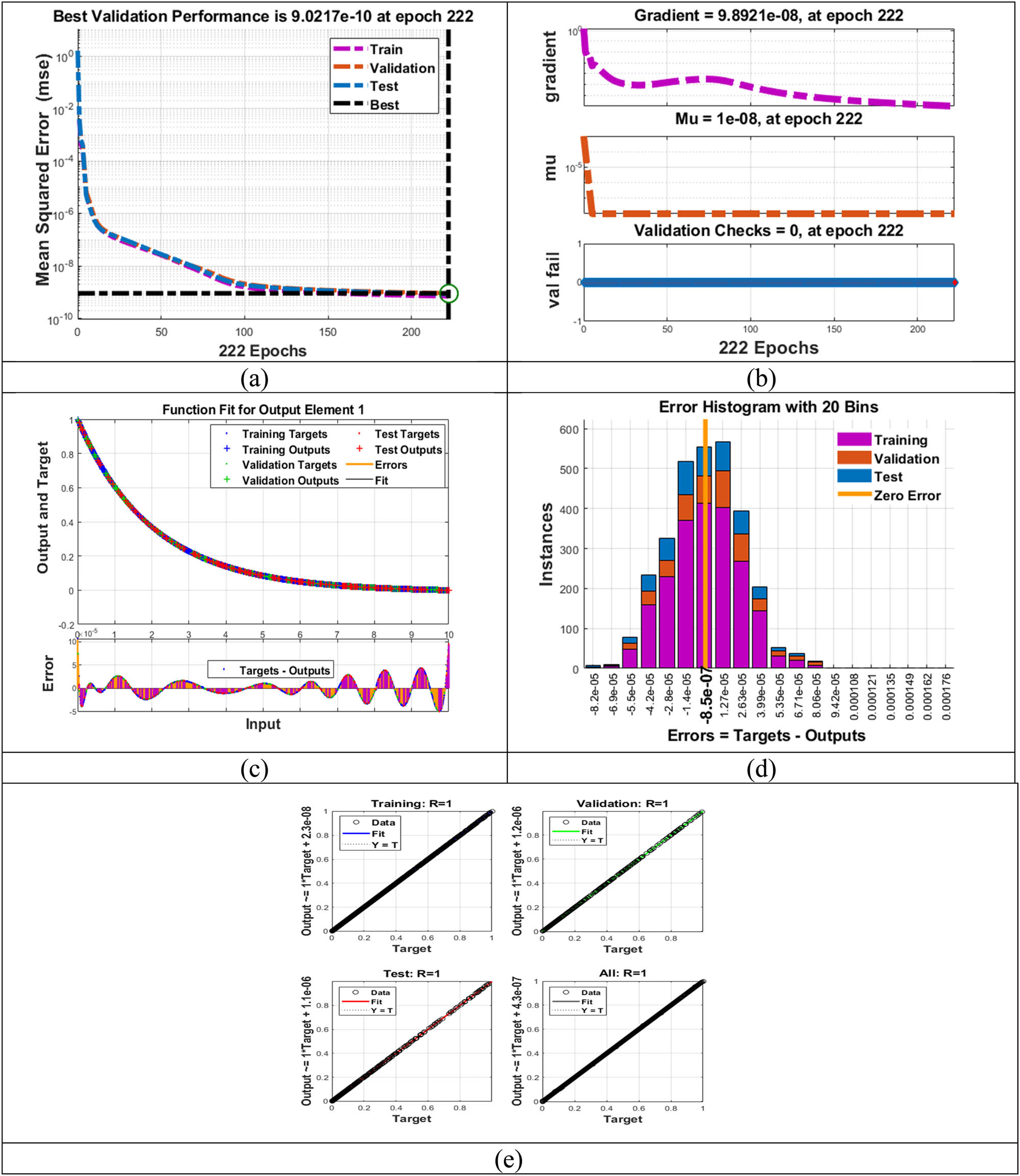
Regression analysis plots, mean square error (MSE), and error histograms are used to validate the performance of the LMLA-BPNN.
The statistical findings determine the numerical values of the proposed LMLA-BPNN for solving the TPD-CNF.

2 Mathematical structure of the problem

We consider a 3-D incompressible and laminar flow of Casson nanofluid induced by a nonlinear extending sheet embedded into TPD. Let u w = ( x + y ) n = v w be the uniform velocity in which the sheet is moving in x _ , y _ directions, respectively, with a and n > 0 which are constants. The symbols T = T ∞ and T = T w represent the free stream temperature and wall temperature of the fluid at the nonlinearly stretching sheet, respectively. C = C ∞ and C = C w are the ambient concentration and nanoparticle fraction concentration at the nonlinearly stretching sheet as the value of z → ∞ . The constitutive state of equation for an isotropic and incompressible laminar flow of the Casson fluid is given as follows:

(a) τ i j = 2 μ B + P y 2 π e i j , π ≥ π c , 2 μ B + P y 2 π c e i j , π < π c .

where τ i j is the Cauchy stress tensor, e i j is the ( i , j ) th component of the strain rate or deformation rate, π = e i j e i j represents the coefficients of strain in product form, π c and μ B are used in non-Newtonian model and is the critical value of π and the plastic dynamic viscosity, respectively. P y indicates the yield stress of the fluid. The physical description of the problem can be visualized in Figure 1.

Figure 1

Geometry of the problem.

The mathematical model using the above assumptions [66–68] are as follows:

(1) u x + v y + w z = 0 ,

(2) u u x + v u y + w u z = 1 + 1 β υ nf u z z ,

(3) u v x + v v y + w v z = 1 + 1 β υ nf v z z ,

(4) u T x + v T y + w T z = k nf ( ρ c p ) nf T z z ,

(5) u C x + v C y + w C z = D nf C z z − ( V T ( C − C ∞ ) ) z .

where u , v , w ( m s − 1 ) are the components of velocity along x , y , z ( m ) directions, respectively. β ( − ) is the Casson parameter, ν = μ ρ ( m 2 s − 1 ) is kinematic viscosity, ( μ = kg m − 1 s − 1 ) is the dynamic viscosity, ( ρ = kg m − 3 ) is the density, ( k = kg ms − 3 K − 1 ) is the thermal conductivity, ( c p = m 2 s − 2 K − 1 ) is the specific heat, ( D = m 2 s − 1 ) is the diffusivity, and ( V T = m s − 1 ) is the thermophoretic velocity.

The boundary conditions are as follows [68,69],

(6) u = u w , v = v w , T = T w , C = C w , w = 0 at z = 0 ,

(7) u → 0 , v → 0 , T → T ∞ , C → C ∞ as z → ∞ .

Here the term V T is defined as

(8) V T = − K 1 υ nf T r T z ,

where T r is the reference temperature and K 1 is the thermophoretic coefficient [66].

In order to solve the governing model, the suitable non-dimensional similarity transformations are introduced as follows [68,69]:

(9) u = a ( x + y ) n f ' ( η ) , v = a ( x + y ) n g ' ( η ) , w = − ( f ' ( η ) + g ' ( η ) ) n − 1 2 η + ( f ( η ) + g ( η ) ) n + 1 2 ( x + y ) n − 1 2 a ν f , η = ( x + y ) n − 1 2 a ν f z , T = T ∞ + θ ( η ) ( T w − T ∞ ) , C = C ∞ + χ ( η ) ( C w − C ∞ ) .

By finding all the components of Eqs. (1)–(5), we get the results in the form of Eqs. (10)–(33), which are

(10) u x = ∂ u ∂ x = ∂ ∂ x ( a ( x + y ) n f ' ( η ) ) ,

(11) u x = ∂ u ∂ x = a n − 1 2 η ( x + y ) n − 1 f ″ ( η ) + a n ( x + y ) n − 1 f ′ ( η ) ,

(12) v y = ∂ v ∂ y = ∂ ∂ y ( a ( x + y ) n g ' ( η ) ) ,

(13) v y = ∂ v ∂ y = a n − 1 2 η ( x + y ) n − 1 g ″ ( η ) + a n ( x + y ) n − 1 g ′ ( η ) ,

(14) w z = ∂ w ∂ z = ∂ ∂ z − ( f ' ( η ) + g ' ( η ) ) n − 1 2 η + ( f ( η ) + g ( η ) ) n + 1 2 ( x + y ) n − 1 2 a ν f ,

(15) w z = ∂ w ∂ z = − n − 1 2 ( x + y ) n − 1 an f ″ ( η ) − n − 1 2 ( x + y ) n − 1 a f ′ ( η ) − n − 1 2 ( x + y ) n − 1 a η g ″ ( η ) − n − 1 2 ( x + y ) n − 1 a g ′ ( η ) − n + 1 2 ( x + y ) n − 1 a f ′ ( η ) − n + 1 2 ( x + y ) n − 1 a g ′ ( η ) ,

(16) u x + v y + w z = a n − 1 2 η ( x + y ) n − 1 f ″ ( η ) + a n ( x + y ) n − 1 f ′ ( η ) + a n − 1 2 η ( x + y ) n − 1 g ( η ) + a n ( x + y ) n − 1 g ′ ( η ) + − n − 1 2 ( x + y ) n − 1 a η f ″ ( η ) − n − 1 2 ( x + y ) n − 1 a f ′ ( η ) − n − 1 2 ( x + y ) n − 1 a η g ″ ( η ) − n − 1 2 ( x + y ) n − 1 a g ′ ( η ) − n + 1 2 ( x + y ) n − 1 a f ′ ( η ) − n + 1 2 ( x + y ) n − 1 a g ′ ( η ) ,

(17) u x + v y + w z = a n − 1 2 η ( x + y ) n − 1 f ″ ( η ) + a n ( x + y ) n − 1 f ′ ( η ) + a n − 1 2 η ( x + y ) n − 1 g ″ ( η ) + a n ( x + y ) n − 1 g ′ ( η ) + − n − 1 2 ( x + y ) n − 1 a η f ″ ( η ) − n − 1 2 ( x + y ) n − 1 a f ′ ( η ) − n − 1 2 ( x + y ) n − 1 a η g ″ ( η ) − n − 1 2 ( x + y ) n − 1 a g ′ ( η ) − n + 1 2 ( x + y ) n − 1 a f ′ ( η ) − n + 1 2 ( x + y ) n − 1 a g ′ ( η ) ,

(18) u x + v y + w z = n − 1 2 a η ( x + y ) n − 1 f ″ ( η ) + ( x + y ) n − 1 a n f ′ ( η ) + n − 1 2 a η ( x + y ) n − 1 g ″ ( η ) + a n ( x + y ) n − 1 g ′ ( η ) − n − 1 2 ( x + y ) n − 1 a η f ″ ( η ) − ( x + y ) n − 1 a n f ′ ( η ) − n − 1 2 ( x + y ) n − 1 a η g ″ ( η ) − ( x + y ) n − 1 a n g ′ ( η ) , u x + v y + w z = 0 ,

(19) u y = a n − 1 2 η ( x + y ) n − 1 f ″ ( η ) + n ( x + y ) n − 1 f ′ ( η ) ,

(20) u z = a ( x + y ) 3 n − 1 2 a ν f f ″ ( η ) ,

(21) u z z = a 2 ν f ( x + y ) 2 n − 1 f ‴ ( η ) ,

(22) v x = a n − 1 2 η ( x + y ) n − 1 g ″ ( η ) + n ( x + y ) n − 1 g ′ ( η ) ,

(23) v z = a ( x + y ) 3 n − 1 2 a ν f g ″ ( η ) , v z z = a 2 ν f ( x + y ) 2 n − 1 g ‴ ( η ) ,

(24) v z = a ( x + y ) 3 n − 1 2 a ν f g ″ ( η ) ,

(25) v z z = a 2 ν f ( x + y ) 2 n − 1 g ‴ ( η ) ,

(26) T x = ( T w − T ∞ ) n − 1 2 ( x + y ) − 1 η d θ d η ,

(27) T y = ( T w − T ∞ ) n − 1 2 ( x + y ) − 1 η d θ d η ,

(28) T z = ( T w − T ∞ ) n − 1 2 ( x + y ) n − 1 2 a ν f d θ d η ,

(29) T z z = ( T w − T ∞ ) n − 1 2 a ν f ( x + y ) n − 1 d 2 θ d η 2 ,

(30) C x = ( T w − T ∞ ) n − 1 2 ( x + y ) − 1 η d ϕ d η ,

(31) C y = ( T w − T ∞ ) n − 1 2 ( x + y ) − 1 η d ϕ d η ,

(32) C z = ( T w − T ∞ ) n − 1 2 ( x + y ) n − 1 2 a ν f d ϕ d η ,

(33) C z z = ( T w − T ∞ ) n − 1 2 a ν f ( x + y ) n − 1 d 2 ϕ d η 2 .

By substituting the values of u x , v y , and w z , we get u x + v y + w z = 0 , i.e., Eqs. (1) and (18) are identically satisfied. By adjusting Eqs. (10)–(33) in Eqs. (2)–(7), we get the following non-dimensional system of ODEs:

(34) 1 + 1 β d 3 f d η 3 − ς 1 ς 2 n d f d η d f d η + d g d η − ( f ( η ) + g ( η ) ) n + 1 2 d 2 f d η 2 = 0 ,

(35) 1 + 1 β d 3 g d η 3 − ς 1 ς 2 n d g d η d f d η + d g d η − ( f ( η ) + g ( η ) ) n + 1 2 d 2 g d η 2 = 0 ,

(36) k nf k f d 2 θ d η 2 + Pr ς 3 n + 1 2 ( f ( η ) + g ( η ) ) d θ d η = 0 ,

(37) ς 1 d 2 ϕ d η 2 + Sc n + 1 2 ( f ( η ) + g ( η ) ) d ϕ d η − τ Sc d θ d η d ϕ d η + d 2 θ d η 2 ϕ ( η ) = 0 ,

with

(38) d f d η ( 0 ) d g d η ( 0 ) f ( 0 ) g ( 0 ) θ ( 0 ) ϕ ( 0 ) = 1 1 0 0 1 1 & d f d η ( ∞ ) d g d η ( ∞ ) θ ( ∞ ) ϕ ( ∞ ) = 0 0 0 0 .

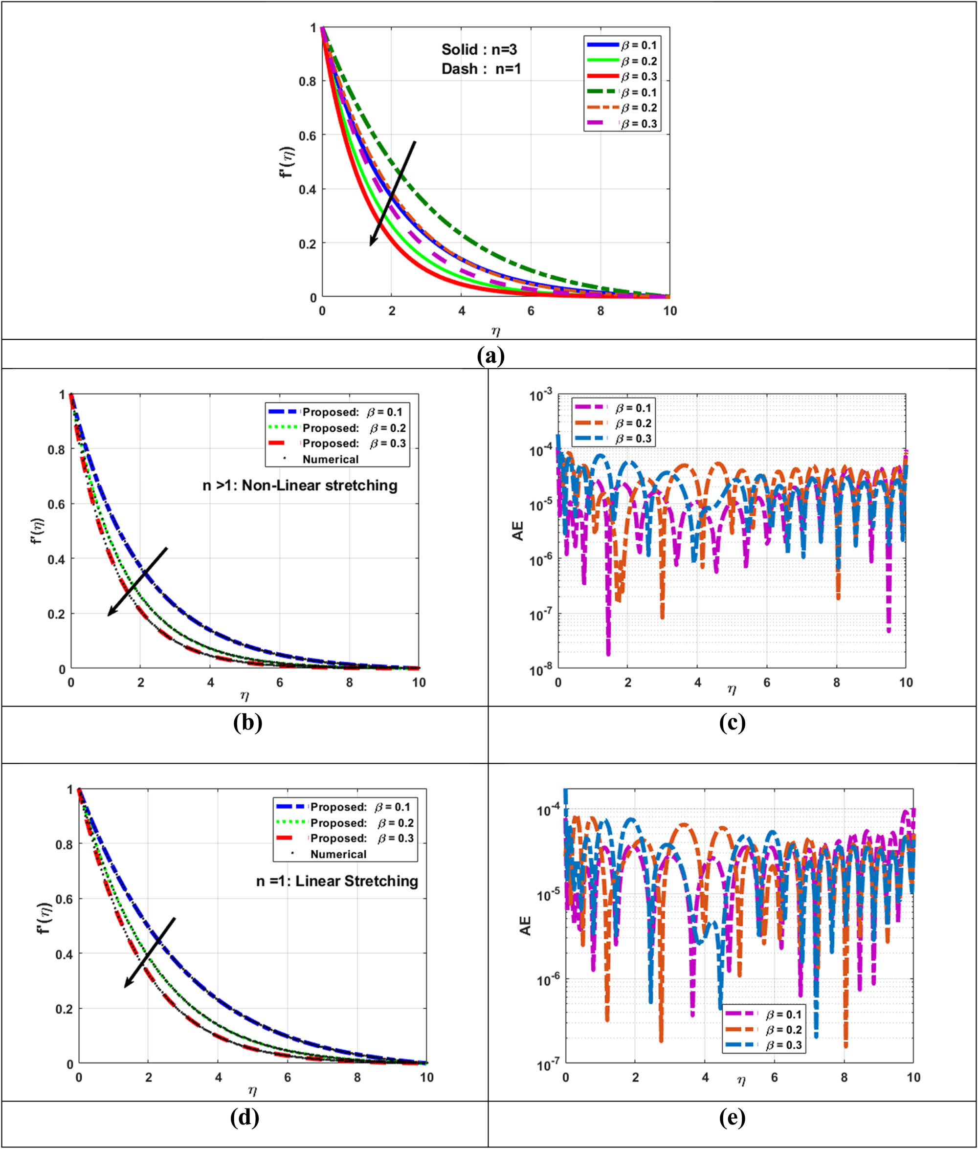
The proposed problem is considered for two cases due to the following assumptions:

n > 1: Nonlinear stretching,
n = 1: Linear stretching,

Where ς 1 = ( 1 − φ ) 2.5 , ς 2 = 1 − φ + φ ρ s ρ f , and ς 3 = 1 − φ + φ ( ρ c p ) s ( ρ c p ) f Sc = v f D f → Schmidt number, Pr = μ f c p f k f → Prandtl number, and τ = − k 1 ( T w − T ∞ ) T r → thermophoretic parameter.

The thermophysical properties of nanofluids in Table 1 are given as follows [70,71]:

(39) k nf = k s + 2 k f − 2 φ ( k f − k s ) k s + 2 k f + φ ( k f − k s ) × ( k f ) , ( ρ c p ) nf = ( 1 − φ ) ( ρ c p ) f + φ ( ρ c p ) s , μ nf = μ f ( 1 − φ ) 2.5 , ρ nf = ( 1 − φ ) ρ f + φ ρ s , D nf = D f ( 1 − φ ) 2.5 .

Table 1

Thermophysical properties of base fluid and nanoparticles [65]

Physical properties	C 6 H 9 NaO 7 (SA)	Al 2 O 3
Pr	6.55	‒
ρ	988	3,975
c _p	4,175	765
k	0.612	40

3 Modeling ANNs with sigmoid function

Researchers have suggested using the sigmoid activation function as a paradigm for ANNs to solve a variety of issues across numerous fields. To solve the Casson nanofluid model, for example, stochastic techniques and a NN model of the sigmoid function were applied. However, no research has been done on the sigmoid function’s use or study in the Casson nanofluid in the presence of TPD effect. Thus, our goal is to examine the application of sigmoid NNs in the TPD-CNF fluid model. A backpropagation ANNs are designed with mathematical systems for TPD-CNF fluid model, and their strength has a continuous mapping form across the single input, hidden, and outer layers based on LMLA-BPNN. Mathematically, it is structured as follows:

(40) f ( η ) = ∑ i = 1 k p i X ( M i η + Q i ) , d f d η = ∑ i = 1 k p i d d t X ( M i η + Q i ) , d 2 f d η 2 = ∑ i = 1 k p i d 2 d t 2 X ( M i η + Q i ) , d 3 f d η 3 = ∑ i = 1 k p i d 3 d t 3 X ( M i η + Q i ) ,

(41) g ( η ) = ∑ i = 1 k p i X ( M i η + Q i ) , d g d η = ∑ i = 1 k p i d d t X ( M i η + Q i ) , d 2 g d η 2 = ∑ i = 1 k p i d 2 d t 2 X ( M i η + Q i ) , d 3 g d η 3 = ∑ i = 1 k p i d 3 d t 3 X ( M i η + Q i ) ,

(42) θ ( η ) = ∑ i = 1 k p i X ( M i η + Q i ) , d θ d η = ∑ i = 1 k p i d d t X ( M i η + Q i ) , d 2 θ d η 2 = ∑ i = 1 k p i d 2 d t 2 X ( M i η + Q i ) ,

(43) ϕ ( η ) = ∑ i = 1 k p i X ( M i η + Q i ) , d ϕ d η = ∑ i = 1 k p i d d t X ( M i η + Q i ) , d 2 ϕ d η 2 = ∑ i = 1 k p i d 2 d t 2 X ( M i η + Q i ) .

Referring to the same mathematical concept, a sigmoid function is a limited, differentiable real function with a single inflection point and a non-negative derivative. The formula provides an illustration of a sigmoid function f ( η ) = 1 1 + e − η .

The sigmoid function f ( M i η + Q i i ) = 1 1 + e M i η + Q i is employed in Eqs. (40)–(43). Eqs. (44)–(47) take on a new mathematical shape following the application of this function.

(44) f ( η ) = ∑ i = 1 k P i 1 1 + e − ( M i η + Q i ) , d f d η = ∑ i = 1 k P i M i e − ( M i η + Q i ) 1 + e − ( M i η + Q i ) 2 , d 2 f d η 2 = ∑ i = 1 k P i M i 2 2 e − 2 ( M i η + Q i ) 1 + e − ( M i η + Q i ) 3 − e − ( M i η + Q i ) 1 + e − ( M i η + Q i ) 2 , d 3 f d η 3 = ∑ i = 1 k P i M i 2 6 e − 3 ( M i η Q i ) 1 + e − ( M i η + Q i ) 4 − 6 e − 2 ( M i η + Q i ) 1 + e − ( M i η + Q i ) 3 + e − ( M i η + Q i ) 1 + e − ( M i η + Q i ) 2 ,

(45) g ( η ) = ∑ i = 1 k P i 1 1 + e − ( M i η + Q i ) , d g d η = ∑ i = 1 k P i M i e − ( M i η + Q i ) 1 + e − ( M i η + Q i ) 2 , d 2 g d η 2 = ∑ i = 1 k P i M i 2 2 e − 2 ( M i η + Q i ) 1 + e − ( M i η + Q i ) 3 − e − ( M i η + Q i ) 1 + e − ( M i η + Q i ) 2 , d 3 g d η 3 = ∑ i = 1 k P i M i 2 6 e − 3 ( M i η Q i ) 1 + e − ( M i η + Q i ) 4 − 6 e − 2 ( M i η + Q i ) 1 + e − ( M i η + Q i ) 3 + e − ( M i η + Q i ) 1 + e − ( M i η + Q i ) 2 ,

(46) θ ( η ) = ∑ i = 1 k P i 1 1 + e − ( M i η + Q i ) , d θ d η = ∑ i = 1 k P i M i e − ( M i η + Q i ) 1 + e − ( M i η + Q i ) 2 , d 2 θ d η 2 = ∑ i = 1 k P i M i 2 2 e − 2 ( M i η + Q i ) 1 + e − ( M i η + Q i ) 3 − e − ( M i η + Q i ) 1 + e − ( M i η + Q i ) 2 ,

(47) ϕ ( η ) = ∑ i = 1 k P i 1 1 + e − ( M i η + Q i ) , d ϕ d η = ∑ i = 1 k P i M i e − ( M i η + Q i ) 1 + e − ( M i η + Q i ) 2 , d 2 ϕ d η 2 = ∑ i = 1 k P i M i 2 2 e − 2 ( M i η + Q i ) 1 + e − ( M i η + Q i ) 3 − e − ( M i η + Q i ) 1 + e − ( M i η + Q i ) 2 .

The equations define the components of vectors P , M , and Q represented by P i , M i , Q i , respectively. The variables P , M , and Q represent the derivative order and the number of neurons. Eqs. (44)–(47) introduce the sigmoid function f ( M i η + Q i ) = 1 1 + e M i η + Q i as the objective function and its higher derivatives, i.e., third order. Furthermore, these equations include the sigmoid function. Eq. (40) denotes the function f ( η ) and its first, second, and third order derivatives. Eq. (44) denotes the same function f ( η ) and its derivatives after applying the sigmoid function. In the same way, Eqs. (41)–(43) represent the functions g ( η ) , θ ( η ) , and ϕ ( η ) along with their first, second, and third order derivatives. On the other hand, Eqs. (45)–(47) represent the functions g ( η ) , θ ( η ) , ϕ ( η ) , and their derivatives up to 3rd order, after merging the sigmoid function.

4 Formulation of fitness function

The MSE is used as the objective function in our modeling given in Eq. (48).

(48) ε = ε 1 + ε 2 + ε 3 + ε 4 ,

(49) ε 1 = 1 N ∑ i = 1 N 1 + 1 β d 3 f d η 3 − ς 1 ς 2 n d f d η d f d η + d g d η − ( f ( η ) + g ( η ) ) n + 1 2 d 2 f d η 2 2 ,

(50) ε 2 = 1 N ∑ i = 1 N 1 + 1 β d 3 g d η 3 − ς 1 ς 2 n d g d η d f d η + d g d η − ( f ( η ) + g ( η ) ) n + 1 2 d 2 g d η 2 2 ,

(51) ε 3 = 1 N ∑ i = 1 N k nf k f d 2 θ d η 2 + Pr ς 3 n + 1 2 ( f ( η ) + g ( η ) ) d θ d η 2 ,

(52) ε 4 = 1 N ∑ i = 1 N ς 1 d 2 ϕ d η 2 + Sc n + 1 2 ( f ( η ) + g ( η ) ) d ϕ d η − τ Sc d θ d η d φ d η + d 2 θ d η 2 φ ( η ) 2 .

Eq. (48) represents this objective function, where ε corresponds to the MSE, which is the summation of ε 1 , ε 2 , ε 3 , and ε 4 . Eqs. (49)–(52) present the expressions for ε 1 , ε 2 , ε 3 , and ε 4 , respectively.

The MSE is displayed by the above four equations. With the availability of ANN-LMLA-BPNN weights, one must optimize ∈ , the objective function, so that ∈ → 0 in order to solve the TPD-CNF fluid model, based on the previous necessity of the dataset for training, testing, and validation as required in classically supervised NNs, trained via an appropriate optimization method (LMLA-BPNN method).

5 Design methodology/NN modeling

Machine learning algorithms (MLA) have been developed to solve practical issues in many branches of STEM. These MLA may be broken down into one of three groups, depending on the kind of instruction used.

Various algorithms cater to different learning paradigms, including unsupervised learning (ULA), reinforcement learning (RLA), and supervised learning (SLA). There are many similarities between the supervised learning algorithm (SLA) and the way humans learn. Considering that people learn new things through exercising and solving difficulties or by analyzing datasets, this analysis uses SLA to adjust weights based on comparisons and correlations with predetermined output goals. The training sample or training dataset instructs NNs on appropriately modifying their weights. The proper result in SLA is the one that the model is expected to produce, given the input. The approach uses backpropagation of errors to fine-tune the supervision weights of the NNs.

In this section, we quickly examine how the suggested LMLA-BPNN affects the 3-D flow of sodium alginate (SA)-based Casson nanofluid across a stretching sheet (TPD-CNF). A collection of the PDEs) that are converted into ODEs specify TPD-CNF. The numerical scheme and the fluidic issue are used in the differential Eqs. (34)–(38), offering a thorough mathematical technique for repeating findings. Matlab’s “bvp4c” built-in function solves TPD-CNF in five distinct variations by transforming higher-order nonlinear ODEs into first-order ODEs.

(53) ( χ 1 = f ) , ( χ 2 = f ′ ) , ( χ 3 = f ″ ) , ( χ 4 = g ) , ( χ 5 = g ′ ) , ( χ 6 = g ″ ) , ( χ 7 = θ ) , ( χ 8 = θ ′ ) , ( χ 9 = χ ) , ( χ 10 = χ ′ ) , ( χ 1 ′ = χ 2 ) , ( χ 2 ′ = χ 3 ) , ( χ 4 ′ = χ 5 ) ( χ 5 ′ = χ 6 ) ( χ 7 ′ = χ 8 ) , ( χ 9 ′ = χ 10 ) ,

(54) d 3 f d η 3 = 1 1 + 1 β ς 1 ς 2 ( f ( η ) + g ( η ) ) n + 1 2 d 2 f d η 2 − n d f d η d f d η + d g d η , χ 3 ′ = 1 1 + 1 β ς 1 ς 2 n + 1 2 ( χ 1 + χ 4 ) χ 3 − n χ 2 ( χ 2 + χ 5 ) ,

(55) d 3 g d η 3 = 1 1 + 1 β ς 1 ς 2 n d g d η d f d η + d g d η − ( f ( η ) + g ( η ) ) n + 1 2 d 2 g d η 2 , χ 6 ′ = 1 1 + 1 β ς 1 ς 2 n χ 5 ( χ 2 + χ 5 ) − n + 1 2 ( χ 1 + χ 4 ) χ 6 ,

(56) d 2 θ d η 2 = − k f k nf Pr ς 3 n + 1 2 ( f ( η ) + g ( η ) ) d θ d η , χ 8 ′ = − k nf k f Pr ς 3 n + 1 2 ( χ 1 + χ 4 ) χ 8 ,

(57) d 2 φ d η 2 = 1 ς 1 τ Sc d θ d η d φ d η + d 2 θ d η 2 φ ( η ) − Sc n + 1 2 ( f ( η ) + g ( η ) ) d φ d η , χ 10 ′ = 1 ς 1 ( χ ′ 8 χ 9 + χ 10 χ 8 ) τ Sc − Sc n + 1 2 χ 10 ( χ 1 + χ 4 ) ,

(58) ( χ 1 ( 0 ) = 0 ) , ( χ 2 ( 0 ) = 1 ) , ( χ 3 ( 0 ) = λ ) , ( χ 4 ( 0 ) = 0 ) , ( χ 5 ( 0 ) = 1 ) , ( χ 6 ( 0 ) = λ 2 ) , ( χ 7 ( ∞ ) = 1 ) , ( χ 8 ( ∞ ) = λ 3 ) , ( χ 9 ( ∞ ) = 1 ) , ( χ 10 ( ∞ ) = λ 4 ) .

In the “bvp4c” built-in function of Matlab, datasets are produced via the process of the numerical solution by adjusting various non-dimensional parameters. The suggested LMLA-BPNN solver makes use of the “nftool” built-in function included in Matlab’s NN toolbox to solve the modified set of Eqs. (54)–(58) that define the fluidic model that represents TPD-CNF. These equations are used to solve the problem. The LMLA-BPNN takes in new information and stores it as the “strengths” of connections between interneurons. These “strengths” are numerical values that are referred to as “weights” in a three-layers design. When calculating the importance of the yield signal, these weights are used after the test input signal values have been determined.

The “input layer” supplies the network with a pattern, which it then employs to make weighted “connections” to one or more “hidden layers” that are responsible for the actual computation. The result is shown on what is referred to as an “output layer,” which is linked to the hidden layers. The ten different types of highly computational units (neurons) that make up the ANN architecture are connected simultaneously. This was done in order to use the sigmoid activation function to solve the fluidic issue. Figure 2 depicts the sigmoid activation function, which is a nonlinearly smooth S-shaped curve. The input values might be any number between +1 and 0. The block architecture of the procedure may be seen in Figure 3. The hypothesized solution is trained, validated, and tested with the use of the reference dataset by using the LMLA-BPNN that was suggested. For the TPD-CNF fluidic approach, Tables 3–7 provide adequate visual and numerical proof to validate the efficacy, dependability, and converge of the LMLA-BPNN via regression analysis, correctness evaluations, and supervised histogram analysis.

Figure 2

NNs for TPD-3DF-SABCNFSS.

Figure 3

The flow architecture of TPD-CNF.

Table 2

Variant of TPD-CNF

	Physical quantities of our interest-based scenarios
Cases	S-Ⅰ	S-Ⅱ	S-Ⅲ	S-Ⅳ	S-Ⅴ
C-I	β = 0.1	β = 0.1	β = 0.1	τ = 0.1	Sc = 0.8
C-II	β = 0.2	β = 0.2	β = 0.3	τ = 0.3	Sc = 1.2
C-III	β = 0.3	β = 0.3	β = 0.5	τ = 0.5	Sc = 1.5

S represent the scenario and C is for case.

Table 3

Outcomes of LMLA-BPNN for scenario Ⅰ of TPD-CNF

Cases	Training	Validation	Testing	Performance	Gradient	Mu	Epoch	Time (s)
Nonlinear stretching
Ⅰ	2.35 × 10 ‒ 6	8.41 × 10 ‒ 7	2.97 × 10 ‒ 6	1.92 × 10 ‒ 6	5.62 × 10 ‒ 6	1.00 × 10 ‒ 8	174	09
Linear stretching
Ⅰ	5.65 × 10 ‒ 10	5.39 × 10 ‒ 10	5.68 × 10 ‒ 10	5.57 × 10 ‒ 10	9.92 × 10 ‒ 8	1.00 × 10 ‒ 9	131	01

Table 4

Outcomes of LMLA-BPNN for scenario Ⅱ of TPD-CNF

Cases	Training	Validation	Testing	Performance	Gradient	Mu	Epoch	Time (s)
Nonlinear stretching
Ⅰ	8.31 × 10 ‒ 8	7.21 × 10 ‒ 8	8.08 × 10 ‒ 8	8.23 × 10 ‒ 8	1.38 × 10 ‒ 5	1.00 × 10 ‒ 9	225	14
Linear stretching
Ⅰ	2.98 × 10 ‒ 8	1.49 × 10 ‒ 8	2.48 × 10 ‒ 8	2.98 × 10 ‒ 8	3.77 × 10 ‒ 6	1.00 × 10 ‒ 9	1,000	64

Table 5

Outcomes of LMLA-BPNN for scenario Ⅲ of BCF-NFM

Cases	Training	Validation	Testing	Performance	Gradient	Mu	Epoch	Time (s)
Nonlinear stretching
Ⅰ	2.01 × 10 ‒ 9	1.97 × 10 ‒ 9	1.54 × 10 ‒ 9	2.02 × 10 ‒ 9	9.94 × 10 ‒ 8	1.00 × 10 ‒ 9	473	16
Linear stretching
Ⅰ	1.86 × 10 ‒ 9	2.14 × 10 ‒ 9	1.96 × 10 ‒ 9	1.87 × 10 ‒ 9	9.97 × 10 ‒ 8	1.00 × 10 ‒ 9	849	28

Table 6

Outcomes of LMLA-BPNN for scenario Ⅳ of BCF-NFM

Cases	Training	Validation	Testing	Performance	Gradient	Mu	Epoch	Time (s)
Nonlinear stretching
Ⅰ	2.10 × 10 ‒ 9	3.19 × 10 ‒ 9	1.65 × 10 ‒ 9	2.10 × 10 ‒ 9	9.96 × 10 ‒ 8	1.00 × 10 ‒ 9	649	21
Linear stretching
Ⅰ	1.76 × 10 ‒ 9	2.56 × 10 ‒ 9	2.30 × 10 ‒ 9	1.77 × 10 ‒ 9	9.96 × 10 ‒ 8	1.00 × 10 ‒ 9	565	14

Table 7

Outcomes of LMLA-BPNN for scenario Ⅴ of BCF-NFM

Cases	Training	Validation	Testing	Performance	Gradient	Mu	Epoch	Time (s)
Nonlinear stretching
Ⅰ	2.02 × 10 ‒ 9	1.25 × 10 ‒ 9	1.88 × 10 ‒ 9	2.02 × 10 ‒ 9	9.99 × 10 ‒ 8	1.00 × 10 ‒ 9	729	20
Linear stretching
Ⅰ	2.94 × 10 ‒ 9	2.23 × 10 ‒ 9	2.90 × 10 ‒ 9	2.95 × 10 ‒ 9	9.96 × 10 ‒ 8	1.00 × 10 ‒ 9	828	20

With the help of the built-in f function procedures in bvp4c, a reference dataset is offered for the axial acceleration, transversal velocity, energy, and concentration patterns of the proposed LMLA-BPNN for values between 0 and 10, with an equal distance of 0.01 for each of the three instances of the five different circumstances of LMLA-BPNN of TPD-CNF. The gathered datasets are used as benchmarks against which to evaluate ( f ' , g ' , θ , ϕ ( η ) ) . Backpropagated networks, time needed, and total iterations/epochs are shown in Tables 2–7 along with the numerical results of LMLA-BPNN for variants of TPD-CNF in terms of MSE for training data, validation results, test results, and production data (predict output).

6 Results interpretation

Figures 4–8 show the intended LMLA-BPNN results for the TPD-CNF fluid model in different orientations (scenarios) of I–V. For an explanation of the β and Sc cases for f ' ( η ) , the β and τ for g ' ( η ) , and the β for ϕ ( η ) instances, see Figures 4a–8a, which illustrates, using the epochs index, how the learning, verification, and evaluation data converge. The magnificent validation performance attained at epochs 222, 284, 380, 243, and 412 with MSE is almost 9.0217 × 10 − 10 , 4.2643 × 10 − 10 , 1.7189 × 10 − 9 , 1.3366 × 10 − 8 , and 3.7105 × 10 − 9 in times 9, 14, 16, 21, and 20 s for nonlinear stretching portion and 1, 64, 28, 14, and 20 s for linear stretching portion, respectively. All derived lines are judged to have a smooth impact and lead to the stability point, signifying excellent and optimal performance. The performance method will improve with lower MSE values, as seen in the corresponding Tables 3–7 and figures. If the MSE values are low, then the suggested method is likely to perform well and accurately. Figures 4b–8b demonstrate convincingly that LMLA-BPNN is reliable, trustworthy, and effectively convergent when used for problems involving β for f ' ( η ) ; the cases of β for g ' ( η ) ; and finally, the cases of β, Sc, and τ for ϕ ( η ) . Figures 4b–8b show the gradient values for each scenario with the numerical values of the Mu parameters throughout the course of training in another vector recognition. Throughout the training, the procedure is continually upgraded. Depending on the number of inspections and the size of the gradient, the learning is concluded. Gradient will become extremely modest when training gets closer to a minimal level of performance. If the gradient’s magnitude drops below 1.0 × 10 − 5 , the training will end. Mu is the LMLA-BPNN’s adaptive parameter, and it has a direct impact on the convergence of the error. The related results of gradient are 9.8921 × 10 − 8 , 9.8934 × 10 − 8 , 9.8204 × 10 − 8 , 5.2876 × 10 − 7 , and 9.8933 × 10 − 8 , whereas Mu of 1 × 10 − 8 , 1 × 10 − 9 , 1 × 10 − 9 , 1 × 10 − 9 , and 1 × 10 − 9 with epoch of 222, 284, 380, 243, and 412, respectively.

$Figure 4 Visual description of LMLA-BPNN based on variations in β v s f ' ( η ) \beta \hspace{.25em}vs\hspace{.25em}f\text{'}(\eta ) for TPD-CNF. (a) MSE representation, (b) TS’s outputs, (c) CF, (d) DEH, and (e) RA. Note: Transition stat (TS), curve fitting (CF), dynamic error histogram (DEH), regression analysis (RA), mean square error (MSE).$

Figure 4

Visual description of LMLA-BPNN based on variations in β v s f ' ( η ) for TPD-CNF. (a) MSE representation, (b) TS’s outputs, (c) CF, (d) DEH, and (e) RA. Note: Transition stat (TS), curve fitting (CF), dynamic error histogram (DEH), regression analysis (RA), mean square error (MSE).

$Figure 5 Visual description of LMLA-BPNN based on variations in β vs g ' ( η ) \beta \hspace{.25em}\text{vs}\hspace{.25em}g\text{'}(\eta ) for TPD-CNF. (a) MSE representation, (b) TS’s outputs, (c) CF, (d) DEH, and (e) RA.$

Figure 5

Visual description of LMLA-BPNN based on variations in β vs g ' ( η ) for TPD-CNF. (a) MSE representation, (b) TS’s outputs, (c) CF, (d) DEH, and (e) RA.

$Figure 6 Visual description of LMLA-BPNN based on variations in β vs χ ( η ) \beta \hspace{.25em}\text{vs}\hspace{.25em}\chi (\eta ) for TPD-CNF. (a) MSE representation, (b) TS’s outputs, (c) CF, (d) DEH, and (e) RA.$

Figure 6

Visual description of LMLA-BPNN based on variations in β vs χ ( η ) for TPD-CNF. (a) MSE representation, (b) TS’s outputs, (c) CF, (d) DEH, and (e) RA.

$Figure 7 Visual description of LMLA-BPNN based on variations in τ vs χ ( η ) \tau \hspace{.25em}\text{vs}\hspace{.25em}\chi (\eta ) for TPD-CNF. (a) MSE representation, (b) TS’s outputs, (c) CF, (d) DEH, and (e) RA.$

Figure 7

Visual description of LMLA-BPNN based on variations in τ vs χ ( η ) for TPD-CNF. (a) MSE representation, (b) TS’s outputs, (c) CF, (d) DEH, and (e) RA.

$Figure 8 Visual description of LMLA-BPNN based on variations in Sc vs χ ( η ) \text{Sc}\hspace{.25em}\text{vs}\hspace{.25em}\chi (\eta ) for TPD-CNF. (a) MSE representation, (b) TS’s outputs, (c) CF, (d) DEH, and (e) RA.$

Figure 8

Visual description of LMLA-BPNN based on variations in Sc vs χ ( η ) for TPD-CNF. (a) MSE representation, (b) TS’s outputs, (c) CF, (d) DEH, and (e) RA.

The recommended fluidic flow with emphasized modifications and mathematical equations are shown in Figures 4c–8c, with the error standing for the discrepancy between the intended and reference solutions. The visual representation demonstrates that the benchmark predicted output of the recommended LMLA-BPNN solver coincides with the target values for each of the three instances of each of the five situations, proving that the structure for NN building authenticates the exactness of the result. In this scholarly pursuit, Raja et al. [20] adeptly tackled the intricacies of 3-D hybrid nanofluid flow. Employing the Bayesian regularization ANN method, a nuanced numerical solution was achieved. Within this framework, a comprehensive suite of statistical analyses was conducted, grounded in the foundational pillars of training, testing, validation, and performance assessment. The resulting numerical and statistical insights, painstakingly gleaned through methodical progression across the training, testing, and validation phases, cast an illuminating spotlight on the performance of the LM method. These findings unveiled a panorama of promise, indicating that both the Bayesian regularization and LM methods stand as robust contenders for addressing the complexities inherent in the modeling of intricate fluid flow phenomena.

After retraining a NN, an outline of error is shown in Figures 4d–8d, which is an error histogram analysis. Analysis of errors and error values highlight the deviation from expected and desired results. For six unique LMLA-BPNN model circumstances, the average value of the error bin almost compares to zero-line error connecting. For all five scenarios, the comparison error dynamic zero line has nearest errors occurring in the range of − 8.5 × 10 − 7 , 4.38 × 10 − 6 , − 1.3 × 10 − 6 , − 1.7 × 10 − 6 , and − 3.5 × 10 − 6 . The error histogram study demonstrates the LMLA-BPNN algorithm’s validity by showing that the bulk of error values compress over the zero-line. To verify the network’s accuracy, a regression diagram is drawn to show how the inputs, outputs, and desired outcomes are all interconnected. If the training process was flawless, the network’s outputs would be consistent with the desired values. Figures 5e–8e show the outcomes. The data testing, verification, and training processes are shown along the three axes. Each dashed line represents the perfect connection among outcomes, production, and goals. The coefficients of R reflect the connection among the output and the desired value, and the solid line depicts the best-fitting linear regression line. The excellent resolution of the TPD-CNF fluidic model using LMLA-BPNN may be explained by a flawless linear connection between the calculated output and the desired values, demonstrated by regression analysis R = 1.

The following are some benefits of the computational technique and LMLA-BPNN method for fluid flow in TPD-CNF fluid model.

The LMLA-BPNN method, a potent optimization tool, can be used to find an approximation to the solution of a system of nonlinear equations. It can therefore be applied successfully to solve the challenging equations describing TPD-CNF fluid model over a nonlinearly extending sheet.
The computational procedure is based on the Lobatto IIIA (bvp4c Solver), an efficient technique for solving differential equations. This ensures that the equations will have a reliable and accurate solution.
By using the LMLA-BPNN method and computational system, several scenarios with Casson parameters, thermophoretic effects, and Schmidt number have been simulated. Because of this feature, it is a useful tool for studying the fluid dynamics of TPD-CNF model over a nonlinearly extending sheet.

6.1 Effect of Casson parameter

The fundamental aspect of this part is to investigate the impact of numerous non-dimensional constraints on their presented outlines. The transformed ODEs (54)–(57) with BCs (58) are solved with “bvp4c” scheme for the formation of dataset and setting the constraints values as τ = 0.1 , Pr = 6.55 , ϕ = 0.01 , Sc = 0.8 , and, β = 0.5 . Thermophysical properties for base liquid and nanoparticles are described in Table 7. The acquired outcomes visualize the impact of non-dimensional constraints, i.e., Schmidt number ( Sc ) , thermophoretic parameter ( τ ) , Casson parameter ( β ) , and power-law index ( n ) on flow profiles (axial and transverse), and energy and nanofluid concentration profiles. Throughout the simulation process, the power-law index parameter is considered fixed for computation, i.e., n = 1 and n = 3. The axial velocity f ' ( η ) with reference solution is illustrated in Figure 9b and d for Casson parameter ( β ) depicting the behavior of nonlinear ( n > 1 ) and linear stretching ( n = 1 ) , respectively. One essential feature of Casson fluids is the Casson parameter ( β ) . It measures the extent to which the fluid exhibits shear-thinning behavior. A more prominent shear-thinning character is indicated by a higher ( β ) value. Shear-thinning behaviour is the propensity of a fluid to exhibit lower viscosity as the shear rate (or velocity gradient) increases. Within the framework of this investigation, a greater Casson value ( β ) suggests a more noticeable decrease in viscosity as shear rates increase. A steeper velocity gradient is produced close to solid boundaries (such as the stretched surface) by a larger Casson value. This occurs as a result of the shear stress’s superior ability to lower viscosity and promote fluid flow. A fluid that is less shear-thinning and more viscous has a lower Casson value ( β ) . In this instance, there will be more flow resistance shown by the less steep velocity gradient close to the solid surface.

$Figure 9 Assessment of LMLA-BPNN for f ' ( η ) f\text{'}(\eta ) with reference dataset of TPD-CNF. (a) Variation in β \beta for f ' ( η ) f\text{'}(\eta ) , (b) variation in β \beta for f ' ( η ) f\text{'}(\eta ) ( n > 1 ) (n\gt 1) , (c) AE for TPD-CNF, (d) variation in β \beta for f ' ( η ) f\text{'}(\eta ) ( n = 1 ) (n=1) , and (e) AE for TPD-CNF.$

Figure 9

Assessment of LMLA-BPNN for f ' ( η ) with reference dataset of TPD-CNF. (a) Variation in β for f ' ( η ) , (b) variation in β for f ' ( η ) ( n > 1 ) , (c) AE for TPD-CNF, (d) variation in β for f ' ( η ) ( n = 1 ) , and (e) AE for TPD-CNF.

Furthermore, inclination rate is slightly higher for the case n = 3 when compared to n = 1 for transverse velocity g ' ( η ) . The absolute error (AE) analysis for Casson parameter ( β ) when ( n > 1 ) and ( n = 1 ) are presented in Figure 9c and e, respectively. The AE of ( β ) between 10 − 8 − 10 − 3 and 10 − 7 − 10 − 4 indicate the accuracy of LMLA-BPNN.

The relative analysis of transverse component of velocity g ' ( η ) with reference solution is illustrated in Figure 10b and d for Casson parameter ( β ) , which depicts the behavior of nonlinear stretching ( n > 1 ) and linear stretching, ( n = 1 ) respectively. A similar behavior is observed as depicted in the axial velocity profile f ' ( η ) . The AE analysis for Casson parameter ( β ) when ( n > 1 ) and ( n = 1 ) are presented in Figure 10c and d, respectively, to check the accuracy criteria. The AE of ( β ) between 10 − 8 − 10 − 3 and 10 − 9 − 10 − 3 indicate the accuracy of LMLA-BPNN.

$Figure 10 Assessment of LMLA-BPNN for g ' ( η ) g\text{'}(\eta ) with reference dataset of TPD-CNF. (a) Variation in β \beta for g ( η ) g(\eta ) , (b) variation in β \beta for g ' ( η ) g\text{'}(\eta ) ( n > 1 ) (n\gt 1) , (c) AE for TPD-CNF, (d) variation in β \beta for g ( η ) g(\eta ) ( n = 1 ) (n=1) , and (e) AE for TPD-CNF.$

Figure 10

Assessment of LMLA-BPNN for g ' ( η ) with reference dataset of TPD-CNF. (a) Variation in β for g ( η ) , (b) variation in β for g ' ( η ) ( n > 1 ) , (c) AE for TPD-CNF, (d) variation in β for g ( η ) ( n = 1 ) , and (e) AE for TPD-CNF.

The relative analysis of mass transfer profile χ ( η ) with reference solution is illustrated in Figure 11b and d for Casson parameter ( β ) which depicts the behavior of nonlinear stretching ( n > 1 ) and linear stretching ( n = 1 ) , respectively. It is observed that the increase in the numerical domain of Casson parameter ( β ) elevates particle growth, intensifying the improvement of boundary layer thickness. That is why, mass transfer increases. Additionally, the Casson parameter ( β ) affects the Casson nanofluid’s concentration profile. The solute or nanoparticle concentration in the fluid can change depending on the β value. Because of the increased fluid velocity close to the boundary, a larger Casson parameter generally tends to facilitate better mixing and dispersion of nanoparticles in the fluid. Concentration profiles may become more consistent as a result. On the other hand, because the fluid’s shear-thinning property is less noticeable, a lower Casson parameter ( β ) may lead to less effective mixing and concentration gradients close to the solid surface. In conclusion, the velocity and concentration profiles of SA-based Casson nanofluid are significantly shaped by the Casson parameter. Its shear-thinning behavior directly affects the distribution of solutes or nanoparticles and the behavior of the fluid near solid boundaries. Applications that use Casson nanofluids can be designed and optimized with an understanding of these effects. The rate of inclination in nanofluid absorption is slightly faster for ( n = 1 ) when compared to ( n = 3 ) . The AE analysis for Casson parameter ( β ) when ( n > 1 ) and ( n = 1 ) are presented in Figure 11c and d, respectively. The AE of ( β ) between 10 − 7 − 10 − 3 and 10 − 9 − 10 − 3 indicate the accuracy of LMLA-BPNN.

$Figure 11 Assessment of LMLA-BPNN for ϕ ( η ) \phi (\eta ) with reference dataset of TPD-CNF. (a) Variation in β \beta for ϕ ( η ) \phi (\eta ) , (b) variation in β \beta for ϕ ( η ) \phi (\eta ) ( n > 1 ) (n\gt 1) , (c) AE for TPD-CNF, (d) variation in β \beta for ϕ ( η ) \phi (\eta ) ( n = 1 ) (n=1) , and (e) AE for TPD-CNF.$

Figure 11

Assessment of LMLA-BPNN for ϕ ( η ) with reference dataset of TPD-CNF. (a) Variation in β for ϕ ( η ) , (b) variation in β for ϕ ( η ) ( n > 1 ) , (c) AE for TPD-CNF, (d) variation in β for ϕ ( η ) ( n = 1 ) , and (e) AE for TPD-CNF.

6.2 Effect of thermophoretic parameter

The relative analysis of mass transfer profile χ ( η ) with reference solution is illustrated in Figure 12b and d for thermophoretic parameter ( τ ) which depicts the behavior of nonlinear stretching ( n > 1 ) and linear stretching ( n = 1 ) , respectively. A process known as thermophoresis occurs when molecules or particles in a fluid move in response to temperature changes. The concentration profile in the fluid can be significantly impacted by this motion, particularly in areas with temperature gradients or close to solid objects. This explains how the concentration profile is affected by the thermophoretic effect ( τ ) . Particles or molecules in a fluid will undergo thermophoretic mobility when a temperature gradient – that is, areas with varying temperatures – is present. Particles have a natural tendency to migrate from cooler to warmer locations, which propels this motion. Thermophoretic processes can cause concentration gradients at solid surfaces, where temperature differences are frequently observed. Particles tend to concentrate or disperse near the surface in response to the direction of the temperature gradient. Particles may migrate towards the surface, for instance, if the surface is hotter than the surrounding fluid, increasing concentrations close to the solid border. In contrast, particles may migrate away from the surface if the surface is colder, which would lower the concentrations close to the border. The concentration boundary layer is the area close to a solid surface where the concentration of particles changes dramatically. The thickness of this layer can be affected by thermophoretic phenomena. Strong thermophoretic effects may cause the concentration boundary layer to thicken, which would suggest a more noticeable concentration gradient. The mobility of the particles also enhances, which results in a declination in fluid concentration. The AE analysis for thermophoretic parameter ( τ ) when ( n > 1 ) and ( n = 1 ) are presented in Figure 12c and d, respectively, to analyze the convergence region. The AE of ( τ ) between 10 − 7 − 10 − 3 and 10 − 8 − 10 − 2 indicate the accuracy of LMLA-BPNN.

$Figure 12 Assessment of LMLA-BPNN for ϕ ( η ) \phi (\eta ) with reference dataset of TPD-CNF. (a) Variation in τ \tau for ϕ ( η ) \phi (\eta ) , (b) variation in τ \tau for ϕ ( η ) \phi (\eta ) ( n > 1 ) (n\gt 1) , (c) AE for TPD-CNF, (d) variation in τ \tau for ϕ ( η ) \phi (\eta ) ( n = 1 ) (n=1) , and (e) AE for TPD-CNF.$

Figure 12

Assessment of LMLA-BPNN for ϕ ( η ) with reference dataset of TPD-CNF. (a) Variation in τ for ϕ ( η ) , (b) variation in τ for ϕ ( η ) ( n > 1 ) , (c) AE for TPD-CNF, (d) variation in τ for ϕ ( η ) ( n = 1 ) , and (e) AE for TPD-CNF.

6.3 Effect of Schmidt number

The relative analysis of mass transfer profile ϕ ( η ) with reference solution is illustrated in Figures 13b and d for Schmidt number (Sc) which depicts the enhancing behavior of nonlinear stretching ( n > 1 ) and linear stretching ( n = 1 ) , respectively. It is depicted from the plotted figures that concentration profile declines as the Schmidt number ( Sc ) enhances. The ratio of the kinematic viscosity to the coefficient of molecular diffusion is known as Schmidt number ( Sc ) . Higher Schmidt number suggests that viscous effects predominate and that the fluid’s resistance to flow is greater than its mass transporting capacity. In this instance, the fluid’s reduced diffusive ability causes the concentration gradient near solid boundaries to tend to be more apparent. The Schmidt number has an impact on the concentration boundary layer, which is the area close to a solid surface where the concentration of solute or nanoparticles varies dramatically. A thicker concentration boundary layer is the outcome of a higher Schmidt number. This indicates that the solute or nanoparticles must travel a greater distance to diffuse from the surface into the bulk fluid. A high Schmidt number indicates that diffusion is slower than the flow of the fluid. This may result in a concentration profile where the source/sink terms close to the surface or the beginning conditions have a greater influence. Conversely, a low Schmidt number suggests that diffusion happens more quickly than fluid motion, resulting in a concentration profile that closely resembles the fluid velocity profile. The rate of decline is slightly faster in the case of ( n = 3 ) than in the case of ( n = 1 ) for ( τ ) and ( Sc ) . The AE analysis for Schmidt number ( Sc ) when ( n > 1 ) and ( n = 1 ) are presented in Figure 13c and d, respectively. The AE values for ( Sc ) lies between 10 − 7 − 10 − 3 and 10 − 8 − 10 − 3 satisfying the accuracy criteria.

$Figure 13 Assessment of LMLA-BPNN for ϕ ( η ) \phi (\eta ) with reference dataset of TPD-CNF. (a) Variation in Sc \text{Sc} for ϕ ( η ) \phi (\eta ) , (b) variation in Sc \text{Sc} for ϕ ( η ) \phi (\eta ) ( n > 1 ) (n\gt 1) , (c) AE for TPD-CNF, (d) variation in Sc \text{Sc} for ϕ ( η ) \phi (\eta ) ( n = 1 ) (n=1) , and (e) AE for TPD-CNF.$

Figure 13

Assessment of LMLA-BPNN for ϕ ( η ) with reference dataset of TPD-CNF. (a) Variation in Sc for ϕ ( η ) , (b) variation in Sc for ϕ ( η ) ( n > 1 ) , (c) AE for TPD-CNF, (d) variation in Sc for ϕ ( η ) ( n = 1 ) , and (e) AE for TPD-CNF.

7 Conclusion

Utilizing the LM technique in conjunction with a computational framework, i.e., Lobatto IIIA, specifically a type of numerical integration or quadrature method for solving 3-D Casson nanofluid flow in the occurrence of thermophoretic particle deposition over a sheet with a nonlinear extended surface represents a pioneering and innovative approach for addressing this challenging problem. The LM method, recognized as a potent optimization tool, enables the approximation of solutions to a set of nonlinear equations. Meanwhile, at the core of our computational architecture lies the numerical method, a robust technique for tackling higher order differential equations. We apply the LM method to resolve the governing equations governing fluid flow within a 3-D Casson nanofluid flow regime, subsequently utilizing it to determine optimal values for critical parameters. These parameters encompass variables such as fluid velocity, temperature, and concentration profiles. Our computational scheme is employed to solve the governing equations related to fluid flow, temperature, and concentration distribution, thus achieving a comprehensive and robust solution. Our results have implications beyond theoretical advancement. Real-world fluid system optimization can benefit from the insights produced by our NN technique and computational framework. Casson nanofluids based on SA provide an adaptable foundation for a variety of industrial uses. By means of regulated particle deposition, these nanofluids facilitate the creation of personalized, mechanically improved 3D printed components for additive manufacturing. They are perfect for creating precision biomedical devices like medication delivery systems and tissue scaffolds because of their biocompatibility. Moreover, Casson nanofluids improve compactness and heat transfer in heat exchangers and microelectronic cooling. They are useful for better drilling fluids in the oil and gas sector, for product innovation in food processing, for pollutant removal in wastewater treatment, and for functional improvements in textiles and coatings. When nanoparticles are precisely deposited, these nanofluids also help to increase the energy storage performance of devices like lithium-ion batteries and supercapacitors. Expanding the range of our computational approach in subsequent research can take into account more complex fluid processes and the inclusion of other physical components. Our surrogate models can be more precise and effective by utilizing novel NN topologies and training methods. Our study provides a strong foundation for future research and development of computational techniques for thermophoresis particle Casson nanofluid flow, paving the way for future innovation and advancement in fluid dynamics research and applications.

The following are the main points of this article:

The governing relations of the system model are presented in differential system to illustrate the dynamics of the underlying mathematical form of the model.
The bvp4c numerical solver generated reference datasets for the proposed model in a variety of conditions, which were successfully used as inputs and targets of LMLA-BPNN to anticipate approximate solutions for each scenario.
By using the LMLA-BPNN method and computational system, several scenarios with Casson parameters, thermophoretic effects, and Schmidt number have simulated. Because of this feature, it is a useful tool for studying the fluid dynamics of TPD-CNF model over a nonlinearly extending sheet.
The LMLA-BPNN method, a potent optimization tool, can be used to find an approximation to the solution of a system of nonlinear equations. It can therefore be applied successfully to solve the challenging equations describing TPD-CNF fluid model over a nonlinearly extending sheet.
In comparative experiments, the validity of LMLA-BPNN for solving nanofluid models with an accuracy in the range of 10 × 10⁻⁸–10 × 10⁻³ is frequently established, which is based on the MSE of the convergence curves and the absolute difference from the reference results.
Performance evaluation, such as error histogram analyses and the regression index, is used to collaborate the findings for each TPD-CNF scenario.
Apart from the advantages of consistent accuracy, stability, and resilience, the main disadvantage of LMLA-BPNN is the absence of a high-quality dataset for nonlinear systems, which is often confined to certain activities and originations.

Furthermore, several metrics such as flow profile, energy distribution, and nanofluid concentration have been observed across the fluid flow in axial and transverse directions.

The effects of parameters observed for fluidic fields in the presence of nonlinear ( n > 1 ) and linear stretching ( n = 1 ) may be described as follows:

Axial and transverse flow fields slow down when the Casson parameter’s domain go high. Whereas this parameter increases the nanofluid concentration rate.
The thermophoresis effect diminishes the concentration distribution when its values become high. Similarly, Schmidt parameter has opposite behavior on nanofluid concentration distribution.

Acknowledgments

The authors would like to the thank the Prince Sattam bin Abulaziz University project number PSAU/2023/1444.

Funding information: Project number PSAU/2023/1444 founded by the Prince Sattam bin Abulaziz University.
Author contributions: All authors have accepted responsibility for the entire content of this manuscript and approved its submission.
Conflict of interest: The authors state no conflict of interest.

References

[1] Yue C, Han D, Pu W, He W. Parametric analysis of a vehicle power and cooling/heating cogeneration system. Energy. 2016;115:800–10.10.1016/j.energy.2016.09.072Search in Google Scholar

[2] Coco-Enríquez L, Muñoz-Antón J, Martínez-Val JM. New text comparison between CO2 and other supercritical working fluids (ethane, Xe, CH4 and N2) in line-focusing solar power plants coupled to supercritical Brayton power cycles. Int J Hydrogen Energy. 2017;42(28):17611–31.10.1016/j.ijhydene.2017.02.071Search in Google Scholar

[3] Ali N, Teixeira JA, Addali A. A review on nanofluids: fabrication, stability, and thermophysical properties. J Nanomater. 2018;2018:6978130.10.1155/2018/6978130Search in Google Scholar

[4] Choi SU, Eastman JA. Enhancing thermal conductivity of fluids with nanoparticles (No. ANL/MSD/CP-84938; CONF-951135-29). Argonne, IL (United States): Argonne National Lab.(ANL); 1995.Search in Google Scholar

[5] Thomson JJ. Notes on recent research in electricity and magnetism: intended as a sequel to Professor Clerk-Maxwell’s Treatise on electricity and magnetism. Cambridge University Press; 1893.Search in Google Scholar

[6] Xuan Y, Li Q. Heat transfer enhancement of nanofluids. Int J Heat Fluid Flow. 2000;21(1):58–64.10.1016/S0142-727X(99)00067-3Search in Google Scholar

[7] Choi U, Tran T. Experimental studies of the effects of non-Newtonian surfactant solutions on the performance of a shell-and-tube heat exchanger. Recent Dev non-Newtonian Flows Ind Appl. 1991;124:47–52.Search in Google Scholar

[8] Sheikh NA, Chuan Ching DL, Khan I. A comprehensive review on theoretical aspects of nanofluids: Exact solutions and analysis. Symmetry. 2020;12(5):725.10.3390/sym12050725Search in Google Scholar

[9] Hayat T, Khan WA, Abbas SZ, Nadeem S, Ahmad S. Impact of induced magnetic field on second-grade nanofluid flow past a convectively heated stretching sheet. Appl Nanosci. 2020;10(8):3001–9.10.1007/s13204-019-01215-xSearch in Google Scholar

[10] Sreedevi P, Sudarsana Reddy P, Chamkha A. Heat and mass transfer analysis of unsteady hybrid nanofluid flow over a stretching sheet with thermal radiation. SN Appl Sci. 2020;2(7):1–15.10.1007/s42452-020-3011-xSearch in Google Scholar

[11] Ali B, Hussain S, Nie Y, Ali L, Hassan SU. Finite element simulation of bioconvection and Cattaneo-Christov effects on micropolar based nanofluid flow over a vertically stretching sheet. Chin J Phys. 2020;68:654–70.10.1016/j.cjph.2020.10.021Search in Google Scholar

[12] Ibrahim W, Negera M. MHD slip flow of upper-convected Maxwell nanofluid over a stretching sheet with chemical reaction. J Egypt Math Soc. 2020;28(1):1–28.10.1186/s42787-019-0057-2Search in Google Scholar

[13] Ali B, Yu X, Sadiq MT, Rehman AU, Ali L. A finite element simulation of the active and passive controls of the MHD effect on an axisymmetric nanofluid flow with thermo-diffusion over a radially stretched sheet. Processes. 2020;8(2):207.10.3390/pr8020207Search in Google Scholar

[14] Sharma R, Hussain SM, Raju CSK, Seth GS, Chamkha AJ. Study of graphene Maxwell nanofluid flow past a linearly stretched sheet: A numerical and statistical approach. Chin J Phys. 2020;68:671–83.10.1016/j.cjph.2020.10.013Search in Google Scholar

[15] Hussain SM, Sharma R, Mishra MR, Alrashidy SS. Hydromagnetic dissipative and radiative graphene maxwell nanofluid flow past a stretched sheet-numerical and statistical analysis. Mathematics. 2020;8(11):1929.10.3390/math8111929Search in Google Scholar

[16] Kumar B, Srinivas S. Unsteady hydromagnetic flow of Eyring-Powell Nanofluid over an inclined permeable stretching sheet with Joule heating and thermal radiation. J Appl Comput Mech. 2020;6(2):259–70.Search in Google Scholar

[17] Zuhra S, Khan NS, Shah Z, Islam S, Bonyah E. Simulation of bioconvection in the suspension of second grade nanofluid containing nanoparticles and gyrotactic microorganisms. AIP Adv. 2018;8(10):105210.10.1063/1.5054679Search in Google Scholar

[18] Zuhra S, Khan NS, Islam S. Magnetohydrodynamic second-grade nanofluid flow containing nanoparticles and gyrotactic microorganisms. Comput Appl Math. 2018;37(5):6332–58.10.1007/s40314-018-0683-6Search in Google Scholar

[19] Khan NS, Zuhra S, Shah Z, Bonyah E, Khan W, Islam S. Slip flow of Eyring-Powell nanoliquid film containing graphene nanoparticles. AIP Adv. 2018;8(11):115302.10.1063/1.5055690Search in Google Scholar

[20] Raja MAZ, Shoaib M, Khan Z, Zuhra S, Saleel CA, Nisar KS, et al. Supervised neural networks learning algorithm for three dimensional hybrid nanofluid flow with radiative heat and mass fluxes. Ain Shams Eng J. 2022;13(2):101573.10.1016/j.asej.2021.08.015Search in Google Scholar

[21] Tackley PJ. Mantle geochemical geodynamics. Treatise Geophys. 2007;7:437–505.10.1016/B978-044452748-6.00124-3Search in Google Scholar

[22] Zainal NA, Nazar R, Naganthran K, Pop I. Unsteady three-dimensional MHD non-axisymmetric Homann stagnation point flow of a hybrid nanofluid with stability analysis. Mathematics. 2020;8(5):784.10.3390/math8050784Search in Google Scholar

[23] Moravej M, Doranehgard MH, Razeghizadeh A, Namdarnia F, Karimi N, Li LK, et al. Experimental study of a hemispherical three-dimensional solar collector operating with silver-water nanofluid. Sustain Energy Technol Assess. 2021;44:101043.10.1016/j.seta.2021.101043Search in Google Scholar

[24] Ramzan M, Gul H, Chung JD, Kadry S, Chu YM. Significance of Hall effect and Ion slip in a three-dimensional bioconvective tangent hyperbolic nanofluid flow subject to Arrhenius activation energy. Sci Rep. 2020;10(1):1–15.10.1038/s41598-020-73365-wSearch in Google Scholar PubMed PubMed Central

[25] Khan AS, Nie Y, Shah Z, Dawar A, Khan W, Islam S. Three-dimensional nanofluid flow with heat and mass transfer analysis over a linear stretching surface with convective boundary conditions. Appl Sci. 2018;8(11):2244.10.3390/app8112244Search in Google Scholar

[26] Tlili I, Nabwey HA, Ashwinkumar GP, Sandeep N. 3-D magnetohydrodynamic AA7072-AA7075/methanol hybrid nanofluid flow above an uneven thickness surface with slip effect. Sci Rep. 2020;10(1):1–13.10.1038/s41598-020-61215-8Search in Google Scholar PubMed PubMed Central

[27] Yan SR, Toghraie D, Hekmatifar M, Miansari M, Rostami S. Molecular dynamics simulation of water-copper nanofluid flow in a three-dimensional nanochannel with different types of surface roughness geometry for energy economic management. J Mol Liq. 2020;311:113222.10.1016/j.molliq.2020.113222Search in Google Scholar

[28] Waqas H, Imran M, Bhatti MM. Bioconvection aspects in non-Newtonian three-dimensional Carreau nanofluid flow with Cattaneo–Christov model and activation energy. Eur Phys J Spec Top. 2021;230(5):1317–30.10.1140/epjs/s11734-021-00046-8Search in Google Scholar

[29] Alaidrous AA, Eid MR. 3-D electromagnetic radiative non-Newtonian nanofluid flow with Joule heating and higher-order reactions in porous materials. Sci Rep. 2020;10(1):1–19.10.1038/s41598-020-71543-4Search in Google Scholar PubMed PubMed Central

[30] Ghadikolaei SS, Hosseinzadeh K, Ganji DD, Jafari B. Nonlinear thermal radiation effect on magneto Casson nanofluid flow with Joule heating effect over an inclined porous stretching sheet. Case Stud Therm Eng. 2018;12:176–87.10.1016/j.csite.2018.04.009Search in Google Scholar

[31] Usman M, Soomro FA, Haq RU, Wang W, Defterli O. Thermal and velocity slip effects on Casson nanofluid flow over an inclined permeable stretching cylinder via collocation method. Int J Heat Mass Transf. 2018;122:1255–63.10.1016/j.ijheatmasstransfer.2018.02.045Search in Google Scholar

[32] Abbas T, Bhatti MM, Ayub M. Aiding and opposing of mixed convection Casson nanofluid flow with chemical reactions through a porous Riga plate. Proc Inst Mech Eng Part E: J Process Mech Eng. 2018;232(5):519–27.10.1177/0954408917719791Search in Google Scholar

[33] Sharma BK, Gandhi R, Abbas T, Bhatti MM. Magnetohydrodynamics hemodynamics hybrid nanofluid flow through inclined stenotic artery. Appl Math Mech. 2023;44(3):459–76.10.1007/s10483-023-2961-7Search in Google Scholar

[34] Gandhi R, Sharma BK, Mishra NK, Al-Mdallal QM. Computer simulations of EMHD Casson nanofluid flow of blood through an irregular stenotic permeable artery: Application of Koo-Kleinstreuer-Li correlations. Nanomaterials. 2023;13(4):652.10.3390/nano13040652Search in Google Scholar PubMed PubMed Central

[35] Gandhi R, Sharma BK, Al-Mdallal QM, Mittal HVR. Entropy generation and shape effects analysis of hybrid nanoparticles (Cu-Al2O3/blood) mediated blood flow through a time-variant multi-stenotic artery. Int J Thermofluids. 2023;18:100336.10.1016/j.ijft.2023.100336Search in Google Scholar

[36] Gandhi R, Sharma BK. Modelling pulsatile blood flow using casson fluid model through an overlapping stenotic artery with Au-Cu hybrid nanoparticles: Varying viscosity approach. In International workshop of Mathematical Modelling, Applied Analysis and Computation. Cham: Springer Nature Switzerland; 2022, August. p. 155–76.10.1007/978-3-031-29959-9_10Search in Google Scholar

[37] Aman S, Zokri SM, Ismail Z, Salleh MZ, Khan I. Effect of MHD and porosity on exact solutions and flow of a hybrid Casson-nanofluid. J Adv Res Fluid Mech Therm Sci. 2018;44(1):131–9.Search in Google Scholar

[38] Sulochana C, Ashwinkumar GP, Sandeep N. Effect of frictional heating on mixed convection flow of chemically reacting radiative Casson nanofluid over an inclined porous plate. Alex Eng J. 2018;57(4):2573–84.10.1016/j.aej.2017.08.006Search in Google Scholar

[39] Zuhra S, Khan NS, Alam M, Islam S, Khan A. Buoyancy effects on nanoliquids film flow through a porous medium with gyrotactic microorganisms and cubic autocatalysis chemical reaction. Adv Mech Eng. 2020;12(1):1687814019897510.10.1177/1687814019897510Search in Google Scholar

[40] Yu Z, Xu Z, Liu R, Xin R, Li L, Chen L, et al. Prediction of SLM-NiTi transition temperatures based on improved Levenberg–Marquardt algorithm. J Mater Res Technol. 2021;15:3349–56.10.1016/j.jmrt.2021.09.149Search in Google Scholar

[41] Ji Y, Kang Z, Liu X. The data filtering based multiple‐stage Levenberg–Marquardt algorithm for Hammerstein nonlinear systems. Int J Robust Nonlinear Control. 2021;31(15):7007–25.10.1002/rnc.5675Search in Google Scholar

[42] Mahmoudabadi ZS, Rashidi A, Yousefi M. Synthesis of 2D-porous MoS2 as a nanocatalyst for oxidative desulfurization of sour gas condensate: Process parameters optimization based on the Levenberg–Marquardt algorithm. J Environ Chem Eng. 2021;9(3):105200.10.1016/j.jece.2021.105200Search in Google Scholar

[43] Shakibjoo AD, Moradzadeh M, Moussavi SZ, Mohammadzadeh A, Vandevelde L. Load frequency control for multi-area power systems: A new type-2 fuzzy approach based on Levenberg–Marquardt algorithm. ISA Trans. 2022;121:40–52.10.1016/j.isatra.2021.03.044Search in Google Scholar PubMed

[44] Tichavský P, Phan AH, Cichocki A. Krylov-Levenberg-Marquardt algorithm for structured tucker tensor decompositions. IEEE J Sel Top Signal Process. 2021;15(3):550–9.10.1109/JSTSP.2021.3059521Search in Google Scholar

[45] Sajedi R, Faraji J, Kowsary F. A new damping strategy of Levenberg-Marquardt algorithm with a fuzzy method for inverse heat transfer problem parameter estimation. Int Commun Heat Mass Transf. 2021;126:105433.10.1016/j.icheatmasstransfer.2021.105433Search in Google Scholar

[46] Sunori SK, Mittal A, Maurya S, Negi PB, Arora S, Joshi KA, et al. Rainfall prediction using subtractive clustering and Levenberg-Marquardt algorithms. In 2021 5th International Conference on Trends in Electronics and Informatics (ICOEI). IEEE; 2021, June. p. 1458–63.10.1109/ICOEI51242.2021.9452869Search in Google Scholar

[47] Wang M, Xu X, Yan Z, Wang H. An online optimization method for extracting parameters of multi-parameter PV module model based on adaptive Levenberg-Marquardt algorithm. Energy Convers Manag. 2021;245:114611.10.1016/j.enconman.2021.114611Search in Google Scholar

[48] Bekas GK, Alexakis DE, Gamvroula DE. Forecasting discharge rate and chloride content of karstic spring water by applying the Levenberg–Marquardt algorithm. Environ Earth Sci. 2021;80(11):1–12.10.1007/s12665-021-09685-5Search in Google Scholar

[49] Li C, Karamehmedović M, Sherina E, Knudsen K. Levenberg–marquardt algorithm for acousto-electric tomography based on the complete electrode model. J Math Imaging Vis. 2021;63(4):492–502.10.1007/s10851-020-01006-ySearch in Google Scholar

[50] Luo G, Zou L, Wang Z, Lv C, Ou J, Huang Y. A novel kinematic parameters calibration method for industrial robot based on Levenberg-Marquardt and differential evolution hybrid algorithm. Robot Computer-Integr Manuf. 2021;71:102165.10.1016/j.rcim.2021.102165Search in Google Scholar

[51] Zhang C, Li Y, Song G, Dong X. Fast and sensitive non-unit protection method for HVDC grids using Levenberg-Marquardt algorithm. IEEE Trans Ind Electron. 2021.10.1109/TIE.2021.3116570Search in Google Scholar

[52] Habib S, Islam S, Khan Z, Waseem. An evolutionary-based neural network approach to investigate heat and mass transportation by using non-Fourier double-diffusion theories for Prandtl nanofluid under Hall and ion slip effects. Eur Phys J Plus. 2023;138(12):1122.10.1140/epjp/s13360-023-04740-5Search in Google Scholar

[53] Khan Z, Zuhra S, Lone SA, Raizah Z, Anwar S, Saeed A. Intelligent computing Levenberg Marquardt paradigm for the analysis of Hall current on thermal radiative hybrid nanofluid flow over a spinning surface. Numer Heat Transfer Part B: Fundam. 2023;1–29.10.1080/10407790.2023.2274448Search in Google Scholar

[54] Aljuaydi F, Khan Z, Islam S. Numerical investigations of ion slip and Hall effects on Cattaneo-Christov heat and mass fluxes in Darcy-Forchheimer flow of Casson fluid within a porous medium, utilizing non-Fourier double diffusion theories through artificial neural networks ANNs. Int J Thermofluids. 2023;20:100475.10.1016/j.ijft.2023.100475Search in Google Scholar

[55] Raja MAZ, Khan Z, Zuhra S, Chaudhary NI, Khan WU, He Y, et al. Cattaneo-christov heat flux model of 3D Hall current involving biconvection nanofluidic flow with Darcy-Forchheimer law effect: Backpropagation neural networks approach. Case Stud Therm Eng. 2021;26:101168.10.1016/j.csite.2021.101168Search in Google Scholar

[56] Baazeem AS, Arif MS, Abodayeh K. An efficient and accurate approach to electrical boundary layer nanofluid flow simulation: A use of artificial intelligence. Processes. 2023;11(9):2736.10.3390/pr11092736Search in Google Scholar

[57] Umar M, Sabir Z, Zahoor Raja MA, Gupta M, Le DN, Aly AA, et al. Computational intelligent paradigms to solve the nonlinear SIR system for spreading infection and treatment using Levenberg–Marquardt backpropagation. Symmetry. 2021;13(4):618.10.3390/sym13040618Search in Google Scholar

[58] Shoaib M, Raja MAZ, Zubair G, Farhat I, Nisar KS, Sabir Z, et al. Intelligent computing with Levenberg–Marquardt backpropagation neural networks for third-grade nanofluid over a stretched sheet with convective conditions. Arab J Sci Eng. 2021;47:1–19.10.1007/s13369-021-06202-5Search in Google Scholar PubMed PubMed Central

[59] Sabir Z, Botmart T, Raja MAZ, Sadat R, Ali MR, Alsulami AA, et al. Artificial neural network scheme to solve the nonlinear influenza disease model. Biomed Signal Process Control. 2022;75:103594.10.1016/j.bspc.2022.103594Search in Google Scholar

[60] Sabir Z, Raja MAZ, Guerrero Sánchez Y. Solving an infectious disease model considering its anatomical variables with Stochastic numerical procedures. J Healthc Eng. 2022;2022:3774123.10.1155/2022/3774123Search in Google Scholar PubMed PubMed Central

[61] Asif D, Bibi M, Arif MS, Mukheimer A. Enhancing heart disease prediction through ensemble learning techniques with hyperparameter optimization. Algorithms. 2023;16(6):308.10.3390/a16060308Search in Google Scholar

[62] Nawaz Y, Arif MS, Shatanawi W, Nazeer A. An explicit fourth-order compact numerical scheme for heat transfer of boundary layer flow. Energies. 2021;14(12):3396.10.3390/en14123396Search in Google Scholar

[63] Nawaz Y, Arif MS, Abodayeh K. An explicit‐implicit numerical scheme for time fractional boundary layer flows. Int J Numer Methods Fluids. 2022;94(7):920–40.10.1002/fld.5078Search in Google Scholar

[64] Sabir Z, Raja MAZ, Mahmoud SR, Balubaid M, Algarni A, Alghtani AH, et al. A novel design of Morlet wavelet to solve the dynamics of nervous stomach nonlinear model. Int J Comput Intell Syst. 2022;15(1):4.10.1007/s44196-021-00057-2Search in Google Scholar

[65] Nawaz Y, Arif MS, Abodayeh K. A third-order two-stage numerical scheme for fractional Stokes problems: A comparative computational study. J Comput Nonlinear Dyn. 2022;17(10):101004.10.1115/1.4054800Search in Google Scholar

[66] Epstein M, Hauser GM, Henry RE. Thermophoretic deposition of particles in natural convection flow from a vertical plate. J Heat Transfer. 1985;107(2):272–6.10.1115/1.3247410Search in Google Scholar

[67] Butt AS, Tufail MN, Ali A. Three-dimensional flow of a magnetohydrodynamic Casson fluid over an unsteady stretching sheet embedded into a porous medium. J Appl Mech Tech Phys. 2016;57:283–92.10.1134/S0021894416020115Search in Google Scholar

[68] Raju CSK, Sandeep N, Babu MJ, Sugunamma V. Dual solutions for three-dimensional MHD flow of a nanofluid over a nonlinearly permeable stretching sheet. Alex Eng J. 2016;55(1):151–62.10.1016/j.aej.2015.12.017Search in Google Scholar

[69] Khan JA, Mustafa M, Hayat T, Alsaedi A. On three-dimensional flow and heat transfer over a non-linearly stretching sheet: analytical and numerical solutions. PLoS one. 2014;9(9):e107287.10.1371/journal.pone.0107287Search in Google Scholar PubMed PubMed Central

[70] Khan A, Khan D, Khan I, Ali F, Karim FU, Imran M. MHD flow of sodium alginate-based Casson type nanofluid passing through a porous medium with Newtonian heating. Sci Rep. 2018;8(1):8645.10.1038/s41598-018-26994-1Search in Google Scholar PubMed PubMed Central

[71] Devi SA, Devi SSU. Numerical investigation of hydromagnetic hybrid Cu–Al2O3/water nanofluid flow over a permeable stretching sheet with suction. Int J Nonlinear Sci Numer Simul. 2016;17(5):249–57.10.1515/ijnsns-2016-0037Search in Google Scholar

Received: 2023-08-04

Revised: 2023-12-18

Accepted: 2024-01-05

Published Online: 2024-02-23

This work is licensed under the Creative Commons Attribution 4.0 International License.

Articles in the same Issue

https://doi.org/10.1515/phys-2023-0181

Keywords for this article

nanofluid; sodium alginate nanoparticles; Casson fluids; stretched surface; Levenberg; Marquardt backpropagation algorithm; neural networks

Creative Commons

BY 4.0