Nonlinearity modeling for online estimation of industrial cooling fan speed subject to model uncertainties and state-dependent measurement noise
-
Chao-Chung Peng
 ,
Min-Che Tsai
,
Min-Che Tsai

Abstract
This article presents an online speed estimation method for cooling fans in resource-limited embedded systems, considering modeling uncertainties and measurement noise. In the current thriving information technology era, monitoring the state of cooling fans is crucial, particularly for high-performance artificial intelligence server cabinets. Accurate fan speed estimation can be used not only to detect fan abnormalities but also for speed control-related applications. Several challenges arise in developing speed estimation algorithms, including state-dependent measurement noise variance, errors in nonlinear fan dynamic modeling, and uncertainties in parameter estimation. To address these issues, this study employs the unscented Kalman filter (UKF) algorithm, incorporating state-dependent noise modeling and mathematical modeling of parameter uncertainties. An UKF-based parameter update mechanism is developed to compensate for model uncertainties and estimation errors, improving the speed estimation accuracy. Simulation results indicate that the root-mean-square errors are reduced from 1.3393 with the traditional UKF to 0.7485 with the parameter update mechanism. Experimental verifications further validate the effectiveness of the proposed methods and strategies in addressing the challenges associated with speed estimation in cooling fans under uncertainties and noise interference.
1 Introduction
In this era of artificial intelligence and technological advancement, the density of high-performance servers and information technology-related equipment is constantly increasing, placing critical stability demands on these devices. The uninterrupted cooling requirements for servers have become a focal point of attention, leading to a sharp increase in the demand for stable, high-performance cooling fans [1,2].
The cooling fan system, composed of a motor and several rotor blades, represents a popular configuration in cooling systems [3]. The utilization of cooling fans not only optimizes the cost in the development phase but also significantly enhances the heat dissipation efficiency. Therefore, it is often regarded as the primary solution for ambient temperature control [4,5].
In the industrial field, cooling fans are widely employed as heat-dissipation devices for equipment such as computers [6], vehicles [7], and server electronics [8]. Cooling fan systems often require extended operational periods; however, prolonged operation may result in system failures. The primary causes of fan system failures often stem from losses or defects in both electrical and mechanical components, or defects in the manufacturing process [9,10].
These failures in cooling fans could result in equipment overheating or more severe damage, consequently causing server shutdowns and data loss. In light of this, the integration of real-time health monitoring and anomaly detection technologies for fans has become an indispensable component of modern industrial operations [11,12]. It provides an intelligent and proactive approach, ensuring the continuous and efficient operation of fans in critical applications. This approach thereby offers robust support for system stability and reliability.
Recent studies have proposed methodologies for dynamic modeling of cooling fan systems, parameter identification, and online monitoring of fan speeds [13,14]. This is achieved by establishing a virtual fan system, enabling sensor-less online monitoring of fans.
To achieve precise monitoring of fan operations, the measurement of the fan’s state and subsequent data processing are crucial [15,16]. However, this measurement process is often accompanied by noise interference, leading to uncertainties in fan monitoring. These uncertainties result in reduced accuracy, increased risk of false alarms, negative impacts on diagnosis and prediction, and greater complexity in data processing. Therefore, obtaining a clean state signal in real time despite measurement noise is a crucial technological challenge in nonlinear cooling fan systems.
Estimating the internal state of dynamic systems based on a set of noisy observational data has been a significant challenge encountered across diverse fields. For linear systems with known Gaussian white noise, Kalman filter (KF) offers the optimal solution for state estimation mean square error [17]. However, real-world dynamic systems are almost invariably nonlinear, which poses a significant challenge. Nonlinear filters can be broadly categorized into two types [18]. The first type involves linearizing the process and observation models around the previous estimate, treating this preceding estimate as the true state. This approach is exemplified by the extended Kalman filter (EKF) model [19,20]. As indicated in previous research papers [21,22], the EKF can be regarded as providing a first-order approximation, thereby offering suboptimal estimates that may lead to state divergence in certain circumstances. Another type of nonlinear filter employs a set of samples to approximate the distribution of the state. Particle filter is a sequential Monte Carlo algorithm that propagates weighted random particles through a nonlinear system and resamples them based on the likelihood weights of the particles [23,24].
Utilizing a greater number of particles can yield higher precision; however, the computational expenses increase. Additionally, Julier et al. introduced the unscented Kalman filter (UKF) in which they employed the unscented transform (UT). This method involves the propagation of several sigma points through nonlinear functions, reconstructing the Gaussian distribution foundation for a more accurate estimation of nonlinear system behavior [25,26]. Considering the impact of outliers in polluted distributions and the influence of time-varying noise, the performance of the classical UKF significantly deteriorates. Recent research [27] has proposed an adaptive and robust UKF approach using Gaussian process regression-assisted Variational Bayesian to enhance the traditional UKF estimation performance. Zhu and Fu, by integrating UKF with the improved unscented PF algorithm, enhanced the accuracy of assessing the state of health for lithium-ion batteries [28].
Research related to cooling fans has been explored in previous studies [3,13,14]. However, these studies did not deeply address the issues of online fan speed estimation in the presence of both noise and model uncertainties. Additionally, the model parameters of the fan systems in these studies were considered constant. In real-world scenarios, the model uncertainties may not be exactly known, and the associated fans may vary slowly due to changes from long-term use in the environment and operating conditions. Acquiring accurate fan speed is crucial in the process of implementing speed control and online diagnosis.
It is worth noting that recent studies have demonstrated the feasibility of KF techniques in various fan applications, including speed estimation [29], precise control [30], and fault detection [31]. However, there is still a lack of research specifically focused on online speed estimation for nonlinear industrial cooling fans. Therefore, this work aims to develop a framework for accurate online speed estimation of industrial cooling fans, addressing the issues of noise and model uncertainties.
This study utilizes UKF estimation techniques to conduct a detailed case study on online speed estimation for cooling fan systems. We proposed specialized design and improvement strategies for UKF in fan speed estimation to address the fast dynamics and parameter uncertainties often overlooked in previous research [13]. The objective is to achieve real-time state estimation of the fan speed, tackling challenges arising from measurement noise with state-dependent variance, errors in fan nonlinear dynamic modeling, and uncertainties in parameter estimation. The experimental results demonstrate the practical value of the proposed methods in engineering applications.
The specific contributions of this article include: (1) comparative analysis of model derivation and dynamic behavior of cooling fan systems, (2) comparison between nonlinear model speed estimation via EKF and UKF, respectively, (3) analysis and modeling of fan speed measurement noise distribution characteristics, and (4) establishment of a parameter update mechanism under the UKF framework to compensate for parameter estimation errors and model uncertainties, which involves a detailed examination of the dynamic model of cooling fans and provides strategies for setting
The remaining sections of this article are organized as follows: In Section 2, a comprehensive introduction to the cooling fan system is provided, accompanied by a complete derivation of the dynamic model. In Section 3, two nonlinear state estimation methods are reviewed, including an introduction to the EKF and UKF (an analysis of their advantages and disadvantages is presented). Section 4 delves into a case study and numerical simulations of cooling fan speed estimation. This includes noise modeling, a review of fan dynamic models, and an exploration of time-varying parameter uncertainties. Based on these conditions, a parameter update mechanism based on UKF is proposed to enhance the accuracy of online fan speed estimation. The implementation of the proposed method is demonstrated on an experimental platform in Section 5, and the accuracy of speed estimation is compared between the traditional UKF and the proposed UKF with a parameter update mechanism. Experimental results confirm the effectiveness of the proposed method. Finally, Section 6 provides the conclusion of the study.
2 Model description of motor-driven cooling fan
A general industrial cooling fan system consists of a driving circuit, a mechanical rotary structure, and a blade. Suppose that the driving system can be simplified as a DC motor, then the overall system can be briefly illustrated in Figure 1, which contains an electrical driving part, a mechanical rotary part, and an external load part.
![Figure 1
Industrial cooling fan driving system [13].](/document/doi/10.1515/nleng-2024-0049/asset/graphic/j_nleng-2024-0049_fig_001.jpg)
Industrial cooling fan driving system [13].
The governing equation of the electrical driving circuit and the motor mechanism is described as
where
The motor mechanism can be expressed as
in which
where the left-hand side and the right-hand side represent the electric power and mechanical power, respectively. Based on Eq. (3), it reveals that
Since the mechanical dynamics is much slower than the electrical dynamics, the transient response of the electrical circuit can be ignored. As a result,
Based on Eqs. (1)–(3), the system can be simplified to
According to the fan blade aerodynamics in the study of Peng and Li [3], the external load mainly contributes to the drag force induced by the cooling fan. Therefore,
where
in which the equivalent coefficients are defined as follows:
Eq. (7) represents the complete cooling fan dynamics, where
For simplicity, rewrite Eq. (7) as
in which the equivalent parameters are denoted as
Therefore, the physical model of the cooling fan driving system can be described by a nonlinear state equation.
Based on the known physical model of the cooling fan driving system, relevant literature [13] has proposed a recursive low-pass filtering method for parameter identification. This method can accurately estimate the physical model parameters represented by Eq. (10) in real-time.
In the following section, the reduced order model Eq. (9) will be taken as the plant for online speed estimator development. Based on the modeling described in this section, it can be observed that the system involves parameter-dependent as well as parameter-independent model uncertainties. Therefore, the purpose of this article is to estimate the fan speed online in the presence of these modeling errors and measurement noise.
3 Review of Kalman filtering for nonlinear systems
In the process of modeling the cooling fan system, it becomes evident that the physical model of the fan exhibits nonlinear dynamic characteristics. To address the challenges posed by this nonlinearity, this section introduces two commonly used techniques for nonlinear estimation: the EKF and the UT presented with the UKF. Subsequently, a comparative study between the EKF and UKF is presented. To address the problem of the biased estimates resulting from the model uncertainties appear in both the EKF and UKF, a state estimate refinement strategy of UKF is proposed to generate high precision speed estimates.
3.1 EKF
The EKF is a commonly used technique for estimating the state of a nonlinear dynamic system [20]. It extends the traditional KF to handle nonlinearity by linearizing the system dynamics with the Taylor series expansion.
Consider a nonlinear stochastic process model defined by a state transition model and an observation model
where
where
In the EKF, these nonlinear functions are approximated through linearization around the current state estimate, enabling the application of KF principles. The EKF algorithm can be summarized as follows:
| Algorithm 1 EKF | |
|---|---|
| Time update (prediction): | |
| 1: |
|
| 2: |
|
| Measurement update (correction): | |
| 3: |
|
| 4: |
|
| 5: |
|
where
In the prediction step, the algorithm estimates the next state
The EKF utilizes Taylor series expansion to approximate the KF, replacing system matrices with Jacobians. Notably, the EKF is suitable for differentiable models, as it relies on the existence of Jacobians. However, this approach is limited, as it may not work well with non-differentiable or highly nonlinear models, where Jacobians are hard to compute or involve high computational costs. In such cases, linearization may result in larger errors in mean and covariance, potentially leading to divergence of estimates. To better address these issues, UT and UKF will be introduced in the following section.
3.2 UKF
For state estimation of nonlinear models, EKF merely uses one single point to approximate the Gaussian distribution. If the function is highly nonlinear in this local region, linearization may lead to poor estimates. The UKF handles this problem with UT, which uses a set of sample points to describe the Gaussian model and propagates them through the nonlinear system [26].
To utilize the UKF, the weights of the sigma points need to be determined in advance. For every new-coming measurement
and the predicted mean (or the prior estimate of state)
In the correction step, the sigma points are transformed through the observation model,
then the predicted measurement mean and covariance can be calculated as
Note that the predicted covariance Eq. (15) and predicted measurement covariance Eq. (17) are made up of the uncertainty of the UT and the process noise
The cross-covariance matrix between the state space and measurement space is given as
Based on the definition of the error covariance matrix,
Similarly,
Recalling the Kalman gain in EKF,
one can find out that Eqs. (19) and (20) compose the elements in Eq. (21), therefore yielding the Kalman gain as
The state update equation is given as
Substituting Eqs. (20) and (22) into the covariance matrix update in EKF gives the covariance matrix update of UKF
The algorithm of the UKF is summarized as the pseudocode in Algorithm 2.
| Algorithm 2 UKF | |
|---|---|
| Initialize: | |
| 1: | Determine the initial conditions for the state
|
| 2: | Set the parameters for generation of sigma points
|
| 3: | Set the weights of sigma points |
|
|
|
|
Input: New-coming measurement
|
|
|
Output:
|
|
| Begin interrupt routine | |
| Sigma Point Generation: | |
| 4: |
|
| Time update (prediction): | |
| 5: |
|
| 6: |
|
| 7: |
|
| Measurement update (correction): | |
| 8: |
|
| 9: |
|
| 10: |
|
| 11: |
|
| 12: |
|
| 13: |
|
| 14: |
|
| End of interrupt routine | |
In summary, the EKF is suitable for systems with mild non-linearity, while the UKF is more robust and suitable for systems with strong non-linearity. The UKF introduces sigma points to not only directly reflect the system evolution but also comprehensively capture system characteristics. Therefore, when dealing with nonlinear systems, the UKF holds a distinct advantage over the EKF, allowing for more accurate estimation by better capturing the characteristics of system nonlinearities. Therefore, this work integrates the UKF to deal with the modeling nonlinearity in the industrial cooling fan and also proposes a state-dependent measurement covariance update mechanism to enhance the fan speed estimation online.
4 Industrial cooling fan speed estimation
The following simulation is conducted in MATLAB using the Runge–Kutta solver, with a numerical time step size set to 0.0005 s.
To apply the UKF algorithm to the cooling fan model, recall the cooling fan dynamic model in Eq. (9). Now, considering an external disturbance
where
To utilize the UKF, the forward difference method is applied to derive the discrete-time model
where
Based on Eq. (28), the discrete-time model can be written as
The model for UKF can be constructed as follows:
State transition equation:
(31)Observation equation:
(32)State and noise covariance:
(33)For Eq. (33), the covariance matrices
For comparative analysis, the model for EKF is also derived as follows.
The prior estimate:
(34)The Jacobians:
The input signal applies a stair-like excitation signal, as described in the study of Peng and Chen [13], and the sample interval
The system starts from rest, thus
To highlight the superiority of the UKF in estimating cooling fan system speed, the parameters of the nonlinear terms in the physical model were intentionally increased to emphasize the performance of both methods in state estimation under conditions where nonlinear effects are more pronounced. Figure 2 illustrates the speed estimation results using the EKF and UKF algorithms. As magnified in Figure 2 inset, taking a closer look at the transient response as an example, one can observe that the EKF algorithm provides a relatively poor estimation, while the UKF yields a more precise speed estimate. In Figure 3, the estimation error between the results and the ground truth is further presented, with root-mean-square (RMS) errors of 0.5608 and 0.3661 for EKF and UKF, respectively. This clearly demonstrates that when the nonlinearity is significant, the local linearization of EKF fails to fully capture the system’s nonlinear behavior, and the UKF exhibits superior state estimation ability in the presence of nonlinearities.
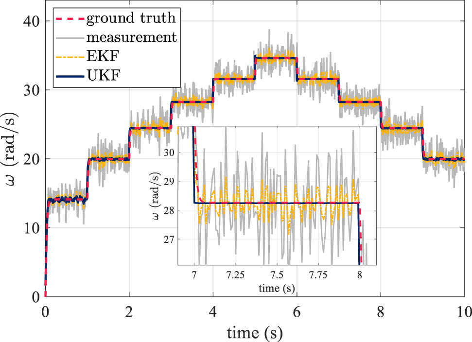
Comparison of speed estimates: EKF vs UKF, with partial enlargement (inset).
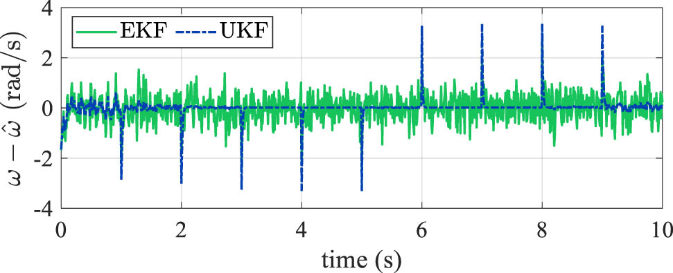
Comparison of the speed estimation error: EKF vs UKF.
Figure 2 highlights the impressive estimation performance, achieved through meticulous adjustment of
To enhance the accuracy of fan speed estimation in the presence of non-uniform Gaussian perturbations, this article proposes strategic approaches. First, a modulation technique for the measurement noise covariance
The ensuing discussion will explore errors related to sensor noise, modeling, and parameter identification, offering valuable insights into strategies for setting
4.1 Measurement noise modeling
In the previous sections, the observation disturbance is assumed to be homoscedastic, that is, the variance remains constant throughout the rotation speed, as shown in Figure 4(a). However, based on the practical experiment observations, it is revealed that the amount of noise becomes larger with a higher fan speed. In this case, the noise of the cooling fan should be assumed to be heteroscedastic, which means that the variance depends on the value of the speed. Figure 4(b) demonstrates that as the value becomes larger, the data points are more widely distributed due to its larger variance, showing the heteroscedasticity of the noise.
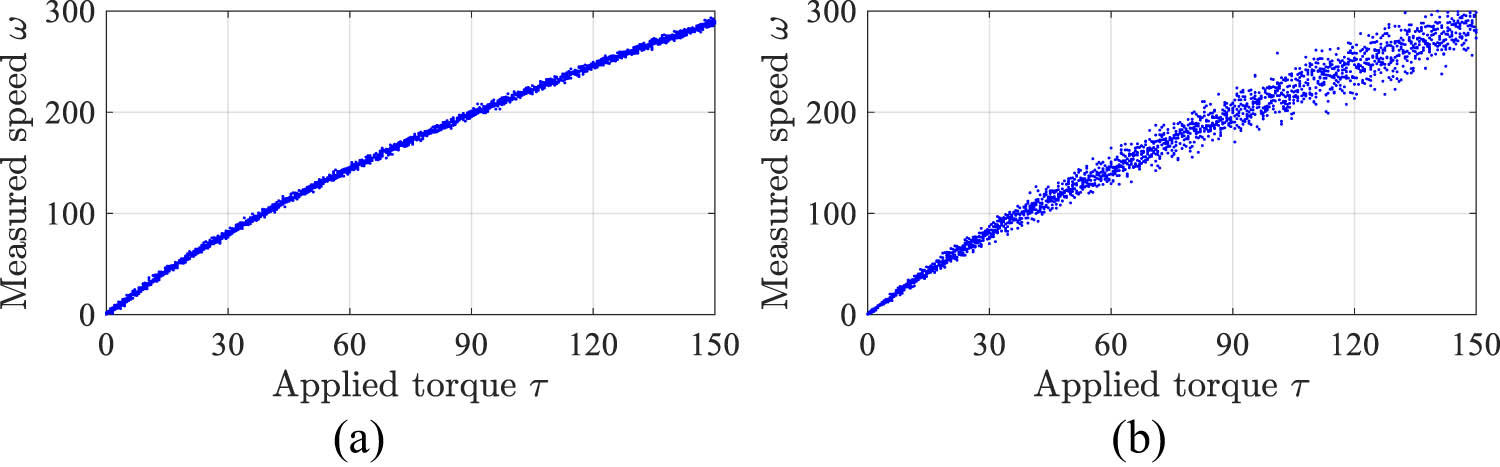
Noise behavior statistical analysis. (a) Homoscedasticity. (b) Heteroscedasticity.
Assume that the standard deviation is a function of speed
where
The fitting problem is fitted into
Monitoring different values of the fan speed, collecting the measured data, and calculating the standard deviations yield
The parameter vector
with a time-varying noise covariance
4.2 Cooling fan modeling error discussion
In a recent study on the estimation of cooling fan parameters [13], the real-time parameter estimation results show that for every stair change in the given input, the estimated values exhibit sharp fluctuations, which mainly results from the error of modeling. Recalling the cooling fan model Eq. (9), the transient response of the electrical dynamics is neglected since its time constant
The system in Eqs. (40) and (41) become relatively complex and, unfortunately, the information of current
As a result, the second-order system is reduced by a first-order nonlinear dynamic equation, where the equivalent equation is expressed as Eq. (7). Note that the equivalent parameters Eq. (8) are based on the fact that the driver dynamics is completely ignored. The model reduction process is described in Section 2.
Since only the fan speed output is available, this work attempts to use Figure 5(b) to replace Figure 5(a) as a reduced-order model for equivalent parameter identification. Note that the equivalent first-order model reduction assumes that the electrical dynamics is much faster than the mechanical fan dynamics. This assumption is reasonable and is going to be illustrated by the following simulation and experimental comparison.
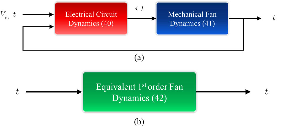
Cooling fan system representation and model reduction. (a) Electrical-circuit-derived second-order fan dynamics. (b) First-order equivalent cooling fan model reduction equivalent representation.
To demonstrate the model mismatch behavior caused by the electrical dynamics,
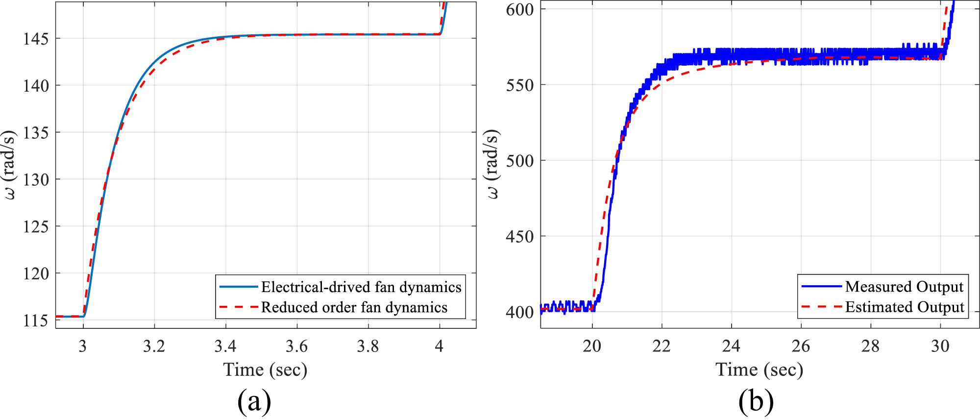
Cooling fan system transient speed response comparison between the electrical-circuit-derived second-order fan dynamics and the reduced order cooling fan representation. (a) Simulation observation. (b) Experimental validation.
Based on the given stair-liked excitation input signal, the simulation results considering Eqs. (40) and (41) show that for an abrupt change in the applied input, the speed response possesses a relatively smooth rising speed within a short period of time. However, the simulation result using Eq. (7) illustrates a sharp rising speed. This slight difference comes from the model reduction or the so-called modeling errors. The qualitative behavior can also be observed from the experiment, as illustrated in Figure 6(b), which further validates the assumption. Consequently, the mismatches between the real system and the equivalent system leads to fluctuation of estimates whenever the applied input changes abruptly.
In conclusion, the main reason this work considered a model reduction is that the current output, generated from Eq. (40), for the general industrial fans in the market is not available. To avoid the use of the current information for cooling fan modeling and fan speed prediction, this work applied a modeling reduction. Figure 6(a) and (b) verify the reasonability of this consideration.
To address this issue and further amend the estimated biases identified in the UKF, the parameter update method with UKF is introduced to refine the speed estimates and to pursue unbiased estimates, and the equivalent system Eq. (7) and the proposed parameter update mechanism are used to make up for the model discrepancy and the parameter identification error.
4.3 UKF with parameter update mechanism
Recalling the cooling fan model in Eqs. (25) and (26), through diverse scenarios encompassing different environments, time frames, and operational conditions, it has been observed from experience that the model parameters of the fan system may undergo slight perturbations, suggesting the potential for time-varying characteristics.
Consequently, we attribute the effects of model uncertainty or disturbances in the fan to the variation of system parameters. Based on this assumption, an online parameter estimation mechanism to enhance unbiased estimation of fan speed is conducted.
Consider the formulation of these time-varying parameters as follows.
where
Thus, the overall system can be described as follows:
Process model:
(44)Observation equation:
(45)of which
Similarly, to utilize the UKF algorithm, the discrete-time model representation of Eq. (44) is derived through the forward difference, given by
(46)and
(47)Concerning the discrete-time model Eq. (46), the actual change rates of uncertainties are unknown in the real world. Fortunately, based on practical experimental statistics, parameter uncertainties can be assumed to be slowly time-varying. Therefore, the practical framework of the UKF for online realization can be modeled as the following transition equation.
Observation equation:
(49)The state vector, the process, and measurement noise are expressed as follows:
and
Note that
The simulation condition is mainly given the same as in the previous instance, where the simulation signal is obtained by the nominal parameters given by
Figure 7 shows the speed estimating results for the general UKF and the proposed method, which evidently shows that with the parameter update mechanism, the biased estimate issue from the parameter uncertainty is eliminated, and the effect of noise is attenuated as well. Figure 8 provides the numerical errors between the estimation results and the ground truth. One can observe that the error of the traditional UKF is not zero-mean and is noisier, while the proposed mechanism alleviates the bias phenomenon and efficiently filters out the noise. The RMS errors are quantified as 1.3393 for the traditional UKF and significantly reduced to 0.7485 for the UKF with the parameter update mechanism.
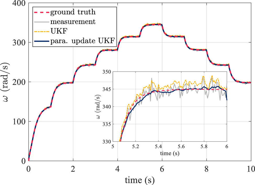
Speed estimate by UKF with the parameter update mechanism.
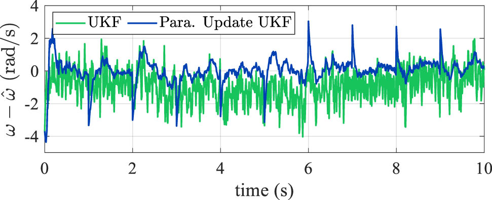
Speed estimation error by UKF with the parameter update mechanism.
Based on simulation results, the conclusion is drawn that under the influence of time-varying uncertainties in perturbation, the traditional UKF, while adjustable through tuning
5 Experimental validation
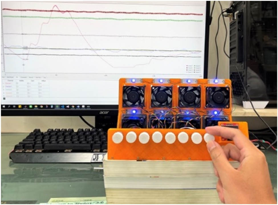
To examine the feasibility of the proposed methods, the algorithms are implemented in an embedded platform for validation. The module of the multi-fan embedded platform is illustrated in Figure 9. The printed circuit board connects the microprocessor Teensy 3.6 with other components, as shown in Figure 9(b) and (c). These components include eight industrial cooling fans, eight knobs for users to manually set the desired speed or control inputs for each fan, eight LEDs indicating the status of each fan, an OLED display showing detailed system information, and two buttons that switch the experiments to different modes. An USB port allows for communication between the PC and Teensy 3.6, which is also the power supplier for the microprocessor.
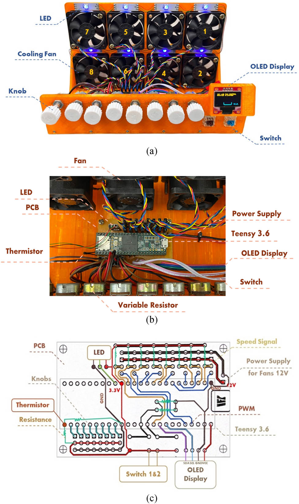
Prototype of the developed cooling fan tray system. (a) Front view of the fan tray system. (b) Microprocessor used for the proposed algorithm realization. (c) PCB layout.
System identification is realized through the application of the low-pass filtering method, as established in the recent research [13]. The equivalent model parameters in Eq. (7) are identified as
5.1 Experiments on R modulation
In preparation for applying UKF algorithms to the cooling fans, the modulation of the covariance
then
Applying a fixed step input, the speed will reach a steady state after 3 s, and the recursions start at this point. The embedded system only needs to store the final value of the recursion and repeat this process for several different levels of fixed input voltages. The relationship between
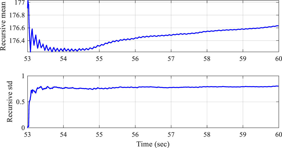
Recursive mean and recursive standard deviation.
Statistical data of fan 1
| PWM (%) | Speed (rps) | Std. | Variance R |
|---|---|---|---|
| 9.9992 | 13.4706 | 0.0514 | 0.0026 |
| 23.3326 | 38.9528 | 0.1599 | 0.0255 |
| 36.6659 | 78.5468 | 0.3203 | 0.1026 |
| 49.9992 | 110.2039 | 0.3951 | 0.1561 |
| 63.3326 | 137.4071 | 0.5812 | 0.3377 |
| 76.6659 | 163.9589 | 0.6823 | 0.4656 |
| 89.9992 | 189.3101 | 0.7070 | 0.4998 |
Based on the assumption of heteroscedasticity and the prescribed formulation, the parameters describing the relationship between the speed and standard deviation can be derived by the least-squares solution, as shown in Figure 11.
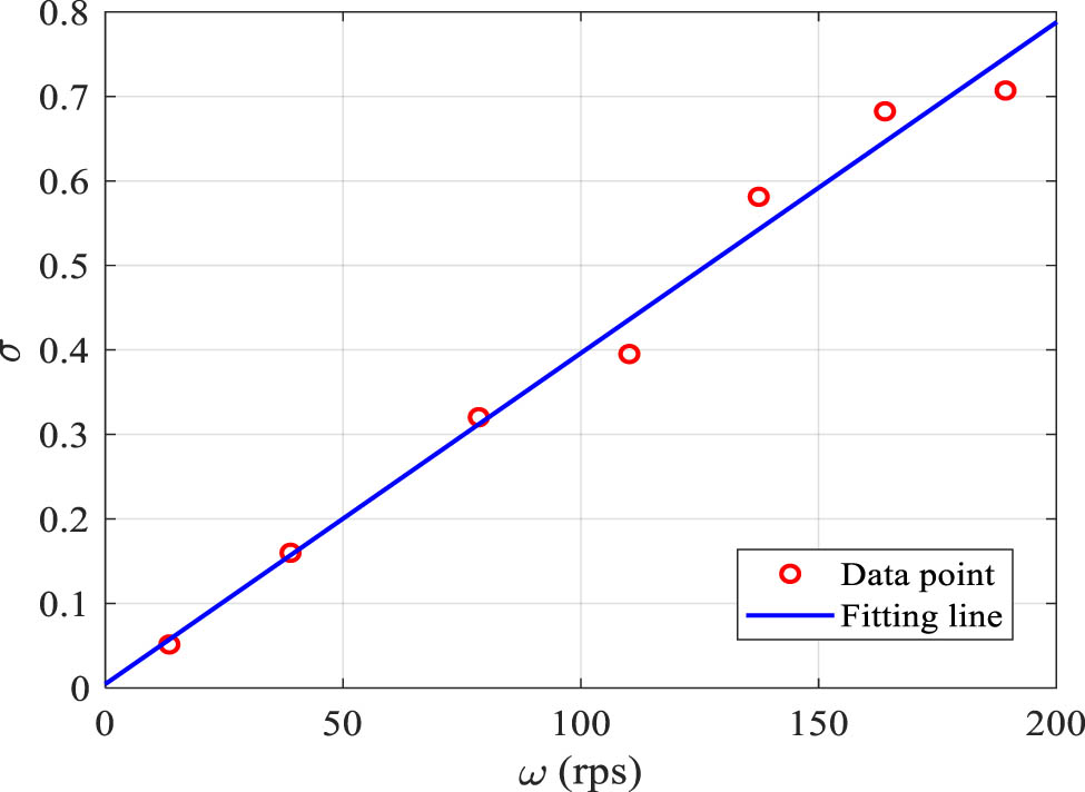
Fitting line for speed and standard deviation of fan 1 with
5.2 Experiments on UKF with parameter update mechanism
The experiments on speed estimation were conducted using two input scenarios: (i) a stair input PWM (Figure 12) and (ii) manual modulation using knob 1 (Figures 13 and 14). In the case of the traditional UKF, a tradeoff arises where a smoother speed requires higher confidence in the mathematical model. However, inherent model and parameter uncertainties in the system lead to a biased speed estimate, as depicted in Figure 12(b) and (c). Conversely, prioritizing an unbiased estimate places greater emphasis on trusting the measurements, which can lead to a decrease in filter effectiveness. As seen in Figure 13(b), the traditional UKF estimate (red line) closely aligns with the measured value (gray line).
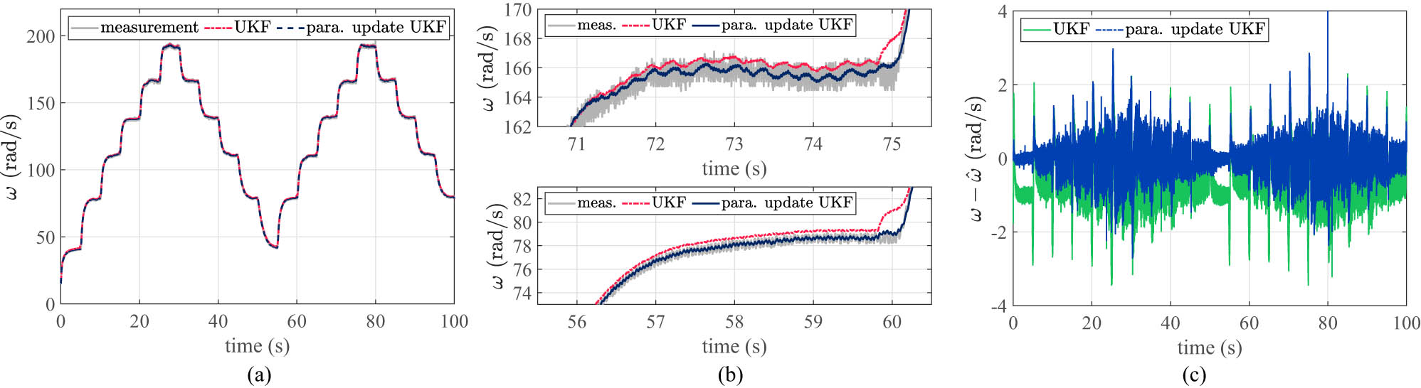
Speed estimates by UKF and UKF with parameter update for stair input. (a) Speed estimation comparison. (b) Responses – partial enlargement. (c) Speed estimation errors.
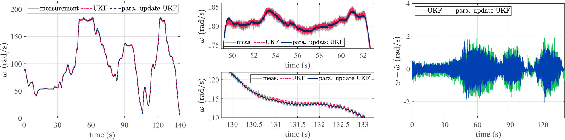
Speed estimates by UKF and UKF with parameter update for manual modulation input. (a) Speed estimation comparison. (b) Responses – partial enlargement. (c) Speed estimation errors.
Manual modulation of fan input commands.
In contrast, the proposed UKF with a parameter update mechanism demonstrates the ability to achieve an unbiased estimate while simultaneously filtering out undesirable noise for both types of input PWM. Figure 13(c) illustrates the corresponding speed estimation errors. Furthermore, Figures 12(c) and 13(c) highlight the proposed method’s capability to mitigate modeling errors that arise from neglecting the electrical driver model. A comparative analysis between Figures 12(b) and 13(b) leads to the conclusion that, for the traditional UKF, the adjustment of
6 Conclusions
This article conducts a detailed case study on real-time speed estimation for cooling fan arrays in source-limited embedded systems, considering modeling uncertainties and the presence of measurement noise. With a focus on practical applications in fan systems, the study proposes a set of strategies to enhance fan speed estimation using the UKF state estimation technique. The discussion encompasses the effect of model reduction, nonlinear model speed estimation, characteristics of speed measurement noise, and the time-varying parameter-dependent uncertainties in fan system models. To address noise during fan measurements, the study utilizes noise modeling to enable automatic modulation of the covariance
-
Funding information: The authors would like to express their deepest gratitude to the National Cheng Kung University and the National Science and Technology Council under project numbers NSTC 112-2221-E-006-104-MY3 and NSTC 113-2218-E-006-021 for their financial support in carrying out this research project.
-
Author contributions: Conceptualization, C. C. Peng; methodology, C. C. Peng; software, M. C. Tsai and T. Y. Chen; validation, M. C. Tsai and T. Y. Chen; formal analysis, C. C. Peng and M. C. Tsai; investigation, C. C. Peng, M. C. Tsai and T. Y. Chen; resources, C. C. Peng; data curation, T. Y. Chen; writing – original draft preparation, M. C. Tsai and T. Y. Chen; writing – review and editing, C. C. Peng; visualization, M. C. Tsai; supervision, C. C. Peng; project administration, C. C. Peng; funding acquisition, C. C. Peng. All authors have accepted responsibility for the entire content of this manuscript and consented to its submission to the journal, reviewed all the results and approved the final version of the manuscript.
-
Conflict of interest: The authors declare no conflicts of interest.
-
Data availability statement: The data that support the findings of this study are available from the corresponding author, C.C. Peng, upon reasonable request.
References
[1] Li C, Li J. Passive cooling solutions for high power server CPUs with pulsating heat pipe technology. Front Energy Res. 2021;9:755019.10.3389/fenrg.2021.755019Search in Google Scholar
[2] Wang Z, Bash C, Tolia N, Marwah M, Zhu X, Ranganathan P. Optimal fan speed control for thermal management of servers. ASME 2009 InterPACK Conference. Vol. 22009, 2009. p. 709–19.10.1115/InterPACK2009-89074Search in Google Scholar
[3] Peng CC, Lin YI, eds. Dynamics modeling and parameter identification of a cooling fan system. 2018 IEEE International Conference on Advanced Manufacturing (ICAM); 2018.10.1109/AMCON.2018.8614957Search in Google Scholar
[4] Staats WL. Active heat transfer enhancement in integrated fan heat sinks [doctoral dissertation]. Cambridge, Massachusetts, USA: Massachusetts Institute of Technology; 2012.Search in Google Scholar
[5] Yoon Y, Kim DR, Lee K-S. Cooling performance and space efficiency improvement based on heat sink arrangement for power conversion electronics. Appl Therm Eng. 2020;164:114458.10.1016/j.applthermaleng.2019.114458Search in Google Scholar
[6] Jian-Hui Z, Chun-Xin Y. Design and simulation of the CPU fan and heat sinks. IEEE Trans CompPackaging Technol. 2008;31(4):890–903.10.1109/TCAPT.2008.2006188Search in Google Scholar
[7] Huang J, Naini SS, Miller R, Rizzo D, Sebeck K, Shurin S, et al. A hybrid electric vehicle motor cooling system – design, model, and control. IEEE Trans Veh Technol. 2019;68(5):4467–78.10.1109/TVT.2019.2902135Search in Google Scholar
[8] Kheirabadi AC, Groulx D. Cooling of server electronics: A design review of existing technology. Appl Therm Eng. 2016;105:622–38.10.1016/j.applthermaleng.2016.03.056Search in Google Scholar
[9] Xijin T, ed. Cooling fan reliability: failure criteria, accelerated life testing, modeling and qualification. RAMS ‘06 Annual Reliability and Maintainability Symposium, 2006; 2006.Search in Google Scholar
[10] Afshar M, Li C, Akin B. Real-time current-based distributed bearing faults detection in small cooling fan motors. IEEE Trans Ind Appl. 2024;60(2):3188–99.10.1109/TIA.2023.3338595Search in Google Scholar
[11] Jin X, Ma EWM, Cheng LL, Pecht M. Health monitoring of cooling fans based on Mahalanobis distance with mRMR feature selection. IEEE Trans Instrum Meas. 2012;61(8):2222–9.10.1109/TIM.2012.2187240Search in Google Scholar
[12] Peng C-C, Chen Y-H. A hybrid neural ordinary differential equation based digital twin modeling and online diagnosis for an industrial cooling fan. Future Internet. 2023;15(9):302.10.3390/fi15090302Search in Google Scholar
[13] Peng C-C, Chen T-Y. A recursive low-pass filtering method for a commercial cooling fan tray parameter online estimation with measurement noise. Measurement. 2022;205:112193.10.1016/j.measurement.2022.112193Search in Google Scholar
[14] Peng CC, Su CY. Modeling and parameter identification of a cooling fan for online monitoring. IEEE Trans Instrum Meas. 2021;70:1–14.10.1109/TIM.2021.3104375Search in Google Scholar
[15] Gong X, Qiao W. Current-based mechanical fault detection for direct-drive wind turbines via synchronous sampling and impulse detection. IEEE Trans Ind Electron. 2015;62(3):1693–702.10.1109/TIE.2014.2363440Search in Google Scholar
[16] Wang XB, Yang ZX, Yan XA. Novel particle swarm optimization-based variational mode decomposition method for the fault diagnosis of complex rotating machinery. IEEE/ASME Trans Mechatron. 2018;23(1):68–79.10.1109/TMECH.2017.2787686Search in Google Scholar
[17] Welch G, Bishop G. An introduction to the Kalman filter. Chapel Hill, United States: University of North Carolina; 1995.Search in Google Scholar
[18] Zhanlue Z, Huimin C, Genshe C, Chiman K, Li XR, eds. Comparison of several ballistic target tracking filters. 2006 American Control Conference; 2006.10.1109/ACC.2006.1656545Search in Google Scholar
[19] Lee JH, Ricker NL, eds. Extended Kalman filter based nonlinear model predictive control. 1993 American Control Conference; 1993.10.23919/ACC.1993.4793207Search in Google Scholar
[20] Ribeiro MI. Kalman and extended kalman filters: Concept, derivation and properties. Inst Syst Robot. 2004;43(46):3736–41.Search in Google Scholar
[21] Wan EA, Merwe RVD, eds. The unscented Kalman filter for nonlinear estimation. Proceedings of the IEEE 2000 Adaptive Systems for Signal Processing, Communications, and Control Symposium (Cat No00EX373); 2000.Search in Google Scholar
[22] Kandepu R, Foss B, Imsland L. Applying the unscented Kalman filter for nonlinear state estimation. J Process Control. 2008;18(7):753–68.10.1016/j.jprocont.2007.11.004Search in Google Scholar
[23] Kwok NM, Gu F, Zhou W, eds. Evolutionary particle filter: re-sampling from the genetic algorithm perspective. 2005 IEEE/RSJ International Conference on Intelligent Robots and Systems; 2005.10.1109/IROS.2005.1545119Search in Google Scholar
[24] Wigren A, Murray L, Lindsten F. Improving the particle filter in high dimensions using conjugate artificial process noise. IFAC-PapersOnLine. 2018;51(15):670–5.10.1016/j.ifacol.2018.09.207Search in Google Scholar
[25] Julier SJ, Uhlmann JK, eds. New extension of the Kalman filter to nonlinear systems. Signal processing, sensor fusion, and target recognition VI. Spie. Conference paper presented at ‘Signal Processing, Sensor Fusion, and Target Recognition VI,’ Vol. 3068, Orlando, FL, United States; 1997.10.1117/12.280797Search in Google Scholar
[26] Julier SJ, Uhlmann JK. Unscented filtering and nonlinear estimation. Proc IEEE. 2004;92(3):401–22.10.1109/JPROC.2003.823141Search in Google Scholar
[27] Lyu X, Hu B, Li K, Chang L. An adaptive and robust UKF approach based on Gaussian process regression-aided variational Bayesian. IEEE Sens J. 2021;21(7):9500–14.10.1109/JSEN.2021.3055846Search in Google Scholar
[28] Zhu F, Fu J. A novel state-of-health estimation for Lithium-Ion battery via unscented Kalman filter and improved unscented particle filter. IEEE Sens J. 2021;21(22):25449–56.10.1109/JSEN.2021.3102990Search in Google Scholar
[29] Tan B, Zhao J, Terzija V, Zhang Y. Decentralized data-driven estimation of generator rotor speed and inertia constant based on adaptive unscented Kalman filter. Int J Electr Power Energy Syst. 2022;137:107853.10.1016/j.ijepes.2021.107853Search in Google Scholar
[30] Lv X, Zhang Y, eds. Extended Kalman filter infusion algorithm design and application characteristics analysis to stochastic closed loop fan speed control of the nonlinear turbo-fan engine. Singapore: Springer Singapore; 2019.10.1007/978-981-13-3305-7_143Search in Google Scholar
[31] Gong CSA, Lee HC, Chuang YC, Li TH, Su CHS, Huang LH, et al. Design and implementation of acoustic sensing system for online early fault detection in industrial fans. J Sens. 2018;2018:4105208.10.1155/2018/4105208Search in Google Scholar
[32] Chen L-H, Peng C-C. Extended backstepping sliding controller design for chattering attenuation and its application for servo motor control. Appl Sci. 2017;7(3):220.10.3390/app7030220Search in Google Scholar
[33] Li Y-R, Peng C-C, Juang J-N. An integral method for parameter identification of a nonlinear robot subject to quantization error. Nonlinear Dyn. 2023;111(24):22419–41.10.1007/s11071-023-09027-zSearch in Google Scholar
[34] Peng C-C, Cheng N-J, Tsai M-C. Application of an output filtering method for an unstable wheel-driven pendulum system parameter identification. Electronics. 2023;12(22):4569.10.3390/electronics12224569Search in Google Scholar
[35] Peng CC. Low-cost embedded real-time handheld vibration smart sensor for industrial equipment onsite defect detection. IEEE Open J Ind Electron Soc. 2021;2:469–78.10.1109/OJIES.2021.3109906Search in Google Scholar
© 2024 the author(s), published by De Gruyter
This work is licensed under the Creative Commons Attribution 4.0 International License.
Articles in the same Issue
- Editorial
- Focus on NLENG 2023 Volume 12 Issue 1
- Research Articles
- Seismic vulnerability signal analysis of low tower cable-stayed bridges method based on convolutional attention network
- Robust passivity-based nonlinear controller design for bilateral teleoperation system under variable time delay and variable load disturbance
- A physically consistent AI-based SPH emulator for computational fluid dynamics
- Asymmetrical novel hyperchaotic system with two exponential functions and an application to image encryption
- A novel framework for effective structural vulnerability assessment of tubular structures using machine learning algorithms (GA and ANN) for hybrid simulations
- Flow and irreversible mechanism of pure and hybridized non-Newtonian nanofluids through elastic surfaces with melting effects
- Stability analysis of the corruption dynamics under fractional-order interventions
- Solutions of certain initial-boundary value problems via a new extended Laplace transform
- Numerical solution of two-dimensional fractional differential equations using Laplace transform with residual power series method
- Fractional-order lead networks to avoid limit cycle in control loops with dead zone and plant servo system
- Modeling anomalous transport in fractal porous media: A study of fractional diffusion PDEs using numerical method
- Analysis of nonlinear dynamics of RC slabs under blast loads: A hybrid machine learning approach
- On theoretical and numerical analysis of fractal--fractional non-linear hybrid differential equations
- Traveling wave solutions, numerical solutions, and stability analysis of the (2+1) conformal time-fractional generalized q-deformed sinh-Gordon equation
- Influence of damage on large displacement buckling analysis of beams
- Approximate numerical procedures for the Navier–Stokes system through the generalized method of lines
- Mathematical analysis of a combustible viscoelastic material in a cylindrical channel taking into account induced electric field: A spectral approach
- A new operational matrix method to solve nonlinear fractional differential equations
- New solutions for the generalized q-deformed wave equation with q-translation symmetry
- Optimize the corrosion behaviour and mechanical properties of AISI 316 stainless steel under heat treatment and previous cold working
- Soliton dynamics of the KdV–mKdV equation using three distinct exact methods in nonlinear phenomena
- Investigation of the lubrication performance of a marine diesel engine crankshaft using a thermo-electrohydrodynamic model
- Modeling credit risk with mixed fractional Brownian motion: An application to barrier options
- Method of feature extraction of abnormal communication signal in network based on nonlinear technology
- An innovative binocular vision-based method for displacement measurement in membrane structures
- An analysis of exponential kernel fractional difference operator for delta positivity
- Novel analytic solutions of strain wave model in micro-structured solids
- Conditions for the existence of soliton solutions: An analysis of coefficients in the generalized Wu–Zhang system and generalized Sawada–Kotera model
- Scale-3 Haar wavelet-based method of fractal-fractional differential equations with power law kernel and exponential decay kernel
- Non-linear influences of track dynamic irregularities on vertical levelling loss of heavy-haul railway track geometry under cyclic loadings
- Fast analysis approach for instability problems of thin shells utilizing ANNs and a Bayesian regularization back-propagation algorithm
- Validity and error analysis of calculating matrix exponential function and vector product
- Optimizing execution time and cost while scheduling scientific workflow in edge data center with fault tolerance awareness
- Estimating the dynamics of the drinking epidemic model with control interventions: A sensitivity analysis
- Online and offline physical education quality assessment based on mobile edge computing
- Discovering optical solutions to a nonlinear Schrödinger equation and its bifurcation and chaos analysis
- New convolved Fibonacci collocation procedure for the Fitzhugh–Nagumo non-linear equation
- Study of weakly nonlinear double-diffusive magneto-convection with throughflow under concentration modulation
- Variable sampling time discrete sliding mode control for a flapping wing micro air vehicle using flapping frequency as the control input
- Error analysis of arbitrarily high-order stepping schemes for fractional integro-differential equations with weakly singular kernels
- Solitary and periodic pattern solutions for time-fractional generalized nonlinear Schrödinger equation
- An unconditionally stable numerical scheme for solving nonlinear Fisher equation
- Effect of modulated boundary on heat and mass transport of Walter-B viscoelastic fluid saturated in porous medium
- Analysis of heat mass transfer in a squeezed Carreau nanofluid flow due to a sensor surface with variable thermal conductivity
- Navigating waves: Advancing ocean dynamics through the nonlinear Schrödinger equation
- Experimental and numerical investigations into torsional-flexural behaviours of railway composite sleepers and bearers
- Novel dynamics of the fractional KFG equation through the unified and unified solver schemes with stability and multistability analysis
- Analysis of the magnetohydrodynamic effects on non-Newtonian fluid flow in an inclined non-uniform channel under long-wavelength, low-Reynolds number conditions
- Convergence analysis of non-matching finite elements for a linear monotone additive Schwarz scheme for semi-linear elliptic problems
- Global well-posedness and exponential decay estimates for semilinear Newell–Whitehead–Segel equation
- Petrov-Galerkin method for small deflections in fourth-order beam equations in civil engineering
- Solution of third-order nonlinear integro-differential equations with parallel computing for intelligent IoT and wireless networks using the Haar wavelet method
- Mathematical modeling and computational analysis of hepatitis B virus transmission using the higher-order Galerkin scheme
- Mathematical model based on nonlinear differential equations and its control algorithm
- Bifurcation and chaos: Unraveling soliton solutions in a couple fractional-order nonlinear evolution equation
- Space–time variable-order carbon nanotube model using modified Atangana–Baleanu–Caputo derivative
- Minimal universal laser network model: Synchronization, extreme events, and multistability
- Valuation of forward start option with mean reverting stock model for uncertain markets
- Geometric nonlinear analysis based on the generalized displacement control method and orthogonal iteration
- Fuzzy neural network with backpropagation for fuzzy quadratic programming problems and portfolio optimization problems
- B-spline curve theory: An overview and applications in real life
- Nonlinearity modeling for online estimation of industrial cooling fan speed subject to model uncertainties and state-dependent measurement noise
- Quantitative analysis and modeling of ride sharing behavior based on internet of vehicles
- Review Article
- Bond performance of recycled coarse aggregate concrete with rebar under freeze–thaw environment: A review
- Retraction
- Retraction of “Convolutional neural network for UAV image processing and navigation in tree plantations based on deep learning”
- Special Issue: Dynamic Engineering and Control Methods for the Nonlinear Systems - Part II
- Improved nonlinear model predictive control with inequality constraints using particle filtering for nonlinear and highly coupled dynamical systems
- Anti-control of Hopf bifurcation for a chaotic system
- Special Issue: Decision and Control in Nonlinear Systems - Part I
- Addressing target loss and actuator saturation in visual servoing of multirotors: A nonrecursive augmented dynamics control approach
- Collaborative control of multi-manipulator systems in intelligent manufacturing based on event-triggered and adaptive strategy
- Greenhouse monitoring system integrating NB-IOT technology and a cloud service framework
- Special Issue: Unleashing the Power of AI and ML in Dynamical System Research
- Computational analysis of the Covid-19 model using the continuous Galerkin–Petrov scheme
- Special Issue: Nonlinear Analysis and Design of Communication Networks for IoT Applications - Part I
- Research on the role of multi-sensor system information fusion in improving hardware control accuracy of intelligent system
- Advanced integration of IoT and AI algorithms for comprehensive smart meter data analysis in smart grids