On theoretical and numerical analysis of fractal--fractional non-linear hybrid differential equations

Shafiullah; Kamal Shah; Muhammad Sarwar; Thabet Abdeljawad

doi:10.1515/nleng-2022-0372

Article Open Access

On theoretical and numerical analysis of fractal--fractional non-linear hybrid differential equations

Shafiullah , Kamal Shah , Muhammad Sarwar and Thabet Abdeljawad

Published/Copyright: March 14, 2024

Published by

Become an author with De Gruyter Brill

Submit Manuscript Author Information

From the journal Nonlinear Engineering Volume 13 Issue 1

Abstract

Recently, fractals and fractional calculus have received much attention from researchers of various fields of science and engineering. Because the said area has been found applicable in modeling various real-world processes and phenomena. Hybrid differential equations (HDEs) play significant roles in mathematical modeling of various processes because the aforesaid equations incorporate different dynamical systems as specific cases. For instance, it is possible to model and describe non-homogeneous physical phenomena on using the said equations. Therefore, this research work is concerned with studying a class of nonlinear hybrid fractal–fractional differential equations. We develop the existence result for the qualitative study using a hybrid fixed point theorem. For the mentioned goal, a fixed point theory for the product of two operators is applied to deduce appropriate conditions for the existence of exactly one solution. Additionally, the stability result based on Ulam–Hyers is also deduced. The said stability results play an important role in numerical investigations. In addition, a numerical method based on Euler procedure is utilized to approximate the solution of the proposed problems. Various computational test problems are given to demonstrate the results. Also, using various fractal–fractional order values, several graphical presentations are given for the examples. The concerned analysis will help in investigating many real-world problems modeled using HDEs with fractal–fractional orders in the near future.

Keywords: fractals and fractional calculus; hybrid problem; existence theory; numerical results

1 Introduction

Calculus of non-integer order has given tremendous popularity because fractional calculus and its applications have been developed so intensively that the areas related to fractional differential equations (FDEs) have attracted a lot of attention [1,2]. Different problems that have studied earlier via ordinary calculus have been generalized by the tools of fractional calculus. For instance, Baleanu et al. [3] have recently published a book, where they established various numerical methods for different models using fractional calculus. In addition, Kilbas et al. [4] have published a comprehensive book on theory and applications of the mentioned area. Rahimy [5] has studied some pertinent applications of FDEs. Magin [6] investigated the models of complex dynamics in biological tissues using the concept of fractional calculus. Jacob et al. [7] have studied various applications of the mentioned area in science and engineering.

Finally, there has been a lot of interest in hybrid differential equations (HDEs), which are nonlinear differential equations perturbed quadratically. The investigations of HDEs are significant since they take into account a number of dynamic systems as special examples. Lakshmikantham and Dhage [8] studied the given problem:

(1) f ( τ ) F ( τ , f ( τ ) ) ′ = V ( τ , f ( τ ) ) , f ( 0 ) = f 0 ,

where F , V : [ 0 , b ] × R → R and w : R → R are the continuous functions and F ( 0 , f ( 0 ) ) ≠ 0 . Here, it is interesting that HDEs have significant applications in mathematical biology, hydrodynamics, signal, and image processing processes. While formulating the concerned phenomenon, we obtain the system of classes of differential equations with hybrid nature. For the mentioned study, many ideas regarding fractional derivatives have been proposed in recent years. Here, we highlight the most well-known varieties, such as Hadamard, Caputo, Liouville, and Caputo-Fabrizio variants, among others. As a result, several fractional operators have created FDEs with distinct structures. Nonetheless, it has long been recognized that accommodating generalized structures of fractional operators that incorporate numerous other operators is the most effective way to discuss such a wide range of fractional operators. Here, we refer to previous studies [9–11].

Complex geometrical structures and irregular shape can be well explained via using a new class of derivatives called fractals. Here, we remark some examples of complex geometry such as shell surfaces and interface problems, which have been studied in Gentilini et al. [12] and Lovadina et al. [13], respectively. In the same way, Norouzi et al. [14] and Shamshuddin et al. [15] have studied the complex geometry of Oldroyd-B visco-elastic fluid flow and nano-fluid flow in pipe. Traditional or ordinary fractional derivatives have inability to accurately describe a range of real-world processes (phenomena) with irregular geometries (structures) and complex geometry. In order to overcome the aforementioned limitations of classical and fractional calculus, academics invented the concept of fractal–fractional derivative. In real-world applications, the mentioned operators have been proved very powerful. Also, the area devoted to fractal geometry is a hot area of research in the last few decades. Also, including fractals in the area of applied analysis opens the door for understanding the recently developed area of analysis on fractals. The said area has been focused on the construction of a Laplacian, which devoted to the Sierpinski gasket and related fractals. The mentioned area has numerous applications. Keeping this in mind, the area of fractional calculus has been extended to a new calculus called fractal–fractional calculus. Various fractional–fractional differential operators have been extended to their fractal form. Recently, a detailed work has been carried out on the said area [16–21].

It should be kept in mind that nonlinear hybrid fractal–fractional differential equations (FFDEs) have not yet been considered under the fractal–fractional calculus concept. To investigate the aforesaid problems, we need some hybrid fixed point results. Dhage [22] established a hybrid fixed point result to deal an ordinary problem. In additions, Dhage’s results were generalized further (for which we refer to previous studies [23–25]). Recently, Venini and Nascimbene [26] have studied a novel fixed-point algorithm utilizing non-linear mixed variational inequalities to harden plasticity. These discoveries have real-world implications for establishing the existence of solutions. Even though it is frequently difficult to compute the fixed point explicitly, these previously described results are acknowledged as powerful tools for creating numerical methods to estimate equation solutions and for estimating the fixed point through computational procedures. Ben Amara et al. [27] deduced a new result for the existence theory based on Boyd–Wong fixed point theorem. With the help of the aforesaid result, we can establish existence results for product of two nonlinear operators in Banach algebras as well for their approximation.

The problem was earlier studied for ordinary derivative in the study by Dhage and Lakshmikantham [8] under the non-homogenous initial condition. They studied only the existence theory of the problem and some comparative analysis. But numerical investigation of such problems has been very rarely considered. Also, under the fractal–fractional concept, such problems have not yet been studied. Due to the significant applications of fractal–fractional operators of integrals and differential type in various scientific disciplines, we consider the class of nonlinear hybrid FFDEs as:

(2) D τ η , ζ 0 F F f ( τ ) F ( τ , f ( τ ) ) = V ( τ , f ( τ ) ) , η , ζ ∈ ( 0 , 1 ] , f ( 0 ) = 0 ,

where F , V : [ 0 , b ] × R → R are continuous functions and F ( 0 , f ( 0 ) ) ≠ 0 . If we put η = ζ = 1 , we obtain Problem (1). Here, we state that the mentioned Problem (2) with initial conditions can formulate many phenomena in various applied disciplines. The concerned applications in analysis for such problems have been given in the studies of Diethelm [28] and Djebali and Sahnoun [29]. We establish the existence results for the proposed problem by using a fixed point theorem for products of two non-linear operators in Banach algebra. Also, we construct the results regarding Ulam–Hyers (UH) stability. The mentioned stability has been deduced around the exact or best approximate solutions for many function equations. More studies have been carried out on the said stability (for instance, refer previous studies [30,31]). Also, to compute exact or analytical solutions for many nonlinear problems is a tedious job. Sometimes it is difficult to compute. Therefore, we search for best approximate solution to nonlinear problems, where we fail to find the exact solution. Therefore, we will extend the usual Euler method to compute the numerical results for our proposed problem also. Numerous test examples are solved, and their solutions have presented graphically using Matlab-16. For theoretical results, we will use the study by Ben Amara et al. [27]; for numerical results, we will extend the method developed in the study by Khan and Atangana [32] for our problem. Here, using the fractal–fractional concept will inform us what is the effect of fractional and fractal calculus on the dynamics of such problems and also what are significant applications of the said calculus in dealing the hybrid dynamical problems.

2 Elementary tools

Let B be a Banach space with norm ‖ . ‖ B and B ( f , r ) be the closed ball. Moreover, for the bounded subset W of B , we denote the norm of a set W by ‖ W ‖ B , which is defined by ‖ W ‖ B = sup { ‖ y ‖ B , y ∈ W } .

Definition 2.1

[32] Assume that f is continuous and fractal-differentiable on the interval ( 0 , T ) with the fractal dimension ζ , then fractal–fractional operator is defined by:

D τ η , ζ 0 F F f ( τ ) = 1 Γ ( 1 − η ) d d τ ζ ∫ 0 τ ( τ − υ ) − η f ( υ ) d υ , 0 < η , ζ ≤ 1 ,

where d f ( s ) d υ ζ = lim τ → s f ( τ ) − f ( υ ) τ ζ − υ ζ is the fractal derivative.

Definition 2.2

[32] Let f be a continuous function on the interval ( 0 , T ) , then

ℐ τ η , ζ 0 F F f ( τ ) = ζ Γ ( η ) ∫ 0 τ ( τ − υ ) η − 1 υ ζ − 1 f ( υ ) d υ ,

which represents the integration in fractal–fractional sense.

Lemma 2.1

[32] The solution of the given problem

D τ η , ζ 0 F F f ( τ ) = z ( t ) , 0 < η , ζ ≤ 1 f ( 0 ) = 0

f ( τ ) = ζ Γ ( η ) ∫ 0 τ υ ζ − 1 ( τ − υ ) η − 1 z ( υ ) d υ .

Definition 2.3

[27] A function S : B → B is called C -Lipschitz if

‖ S ( f ) − S ( f ¯ ) ‖ B ≤ χ ( ‖ f − f ¯ ‖ B ) , ∀ f , f ¯ ∈ B ,

with a non-decreasing function χ : R + → R + obeying χ ( 0 ) = 0 . Moreover, χ is said to be C -function associated with S . Additionally, for χ ( q ) < q , for q > 0 , then S is a non-linear contraction on B .

Theorem 2.4

[27] Let C ≠ ∅ ⊂ B be closed and convex set and S , P : C → B is two operators, such that

S and P are D -Lipschitz with C -functions χ and δ , respectively,
S ( C ) and P ( C ) are bounded,
S ( f ) × P ( f ) ∈ B , for all f ∈ B .

If ‖ S ( C ) ‖ B χ ( q ) + ‖ S ( C ) ‖ B δ ( q ) < q , then there is at most one point f ¯ ∈ B , such that S ( f ¯ ) × P ( f ¯ ) = f ¯ . In addition, for each f 0 ∈ B , the sequence { ( S × P ) n ( f 0 ) } n ∈ N converges to f ¯ .

3 Main results

Here, we provide our main results.

Lemma 3.1

The solution to a class of hybrid FFDEs (2) is given using Lemma 2.1 as

(3) f ( τ ) = ζ Γ ( η ) F ( τ , f ( τ ) ) ∫ 0 τ ( τ − υ ) η − 1 υ ζ − 1 V ( υ , f ( υ ) ) d υ .

Proof

By Definition 2.1, Eq. (2) can be written as:

1 Γ ( 1 − η ) d d τ ζ ∫ 0 τ ( τ − υ ) − η f ( υ ) F ( υ , f ( υ ) ) d υ = V ( τ , f ( τ ) ) ,

which gives

(4) 1 Γ ( 1 − η ) d d τ ∫ 0 τ ( τ − υ ) − η f ( υ ) F ( υ , f ( υ ) ) d υ = ζ τ ζ − 1 V ( τ , f ( τ ) ) .

Now, Eq. (4) can be written as:

(5) D τ η 0 f ( τ ) F ( τ , f ( τ ) ) = ζ τ ζ − 1 V ( τ , f ( τ ) ) .

On using fractional integral operator of order η to Eq. (5) gives

(6) f ( τ ) F ( τ , f ( τ ) ) = ζ Γ ( η ) ∫ 0 τ ( τ − υ ) η − 1 υ ζ − 1 V ( υ , f ( υ ) ) d υ + a 0 t η − 1 .

Using the initial condition in Eq. (2), f ( 0 ) = 0 gives a 0 = 0 , for which Eq. (6) becomes

f ( τ ) = ζ Γ ( η ) F ( τ , f ( τ ) ) ∫ 0 τ ( τ − υ ) η − 1 υ ζ − 1 V ( υ , f ( υ ) ) d υ ,

which is the integral solution of Problem (2).

We set the following assumptions for the upcoming existence result:

F and V are continuous.
Let g , h : J → R be two continuous functions and χ and δ already defined mappings, and f , f ¯ ∈ R , then one has
∣ F ( τ , f ) − F ( τ , f ¯ ) ∣ ≤ g ( τ ) χ ( ∣ f − f ¯ ∣ ) ,

∣ V ( τ , f ) − V ( τ , f ¯ ) ∣ ≤ h ( τ ) δ ( ∣ f − f ¯ ∣ ) .

Throughout this sequel, we denote the closed ball B q = { f ∈ B : ‖ f ‖ B ≤ q } of C ( J ) by Ω , such that Ω ≠ ∅ .

Theorem 3.1

Let the assumptions (A₁) and (A₂) hold, if

M S M P ≤ q and ‖ S ( B ) ‖ B χ ( q ) + ‖ P ( B ) ‖ B δ ( q ) < q , ∀ q > 0 ,

where M S = ( ‖ g ‖ B χ ( ‖ f ‖ B ) + ‖ F ( 0 , f ( 0 ) ) ‖ B ) and

M P = ζ Γ ( η ) β ( η , ζ ) b η + ζ − 1 ( ‖ h ‖ B δ ( ‖ f ‖ B ) + ‖ V ( 0 , f ( 0 ) ) ‖ B ) ,

then Problem (2) has exactly one solution in Ω , where β ( η , ζ ) is the beta function.

Proof

The problem of existence of solution to Eq. (2) can be formulated in the form of fixed point problem f = S ( f ) × P ( f ) , where f ∈ C ( J ) and S and P are the operators given by:

S ( f ( τ ) ) = F ( τ , f ( τ ) )

and P ( f ( τ ) ) = ζ Γ ( η ) ∫ 0 τ ( τ − υ ) η − 1 υ ζ − 1 V ( υ , f ( υ ) ) d υ .

Let f ∈ Ω , and F be C -Lipschitzian function, so one has

∣ F ( τ , f ( τ ) ) − F ( τ ′ , f ( τ ′ ) ) ∣ ≤ ∣ F ( τ , f ( τ ) ) − F ( τ ′ , f ( τ ) ) ∣ + ∣ F ( τ ′ , f ( τ ) ) − F ( τ ′ , f ( τ ′ ) ) ∣ ,

which easily confirms that S assigns Ω into C ( J ) . In addition to using ( A 2 ) , such that τ ′ < τ , and taking

(7) ∣ P ( f ( τ ) ) − P ( f ( τ ′ ) ) ∣ = ζ Γ ( η ) ∫ 0 τ ( τ − υ ) η − 1 υ ζ − 1 V ( υ , f ( s ) ) d υ − ∫ 0 τ ′ ( τ ′ − υ ) η − 1 υ ζ − 1 V ( υ , f ( υ ) ) d υ ≤ ζ Γ ( η ) ∫ 0 τ ′ [ ( τ − υ ) η − 1 − ( τ ′ − υ ) η − 1 ] υ ζ − 1 V ( υ , f ( υ ) ) d υ + ∫ τ ′ τ ( τ − υ ) η − 1 υ ζ − 1 V ( υ , f ( υ ) ) d υ ≤ ζ Γ ( η ) ∫ 0 τ ′ υ ζ − 1 [ ( τ − υ ) η − 1 − ( τ ′ − υ ) η − 1 ] + ∫ τ ′ τ υ ζ − 1 ( τ − υ ) η − 1 ∣ V ( υ , f ( υ ) ) ∣ d υ ≤ ζ Γ ( η ) ∫ 0 τ ′ [ ( τ − υ ) η − 1 − ( τ ′ − υ ) η − 1 ] υ ζ − 1 + ζ Γ ( η ) ∫ τ ′ τ υ ζ − 1 ( τ − υ ) η − 1 ( V ( υ , f ( υ ) ) − V ( 0 , f ( 0 ) ) ∣ + ∣ V ( 0 , f ( 0 ) ) ∣ ) d υ ≤ ζ ( ‖ h ‖ B δ ( q ) + ‖ V ( 0 , f ( 0 ) ) ‖ B ) Γ ( η ) ∫ 0 τ ′ υ ζ − 1 [ ( τ − υ ) η − 1 − ( τ ′ − υ ) η − 1 ] d υ + ∫ τ ′ τ υ ζ − 1 ( τ − υ ) η − 1 d υ = ( ‖ h ‖ B δ ( q ) + ‖ V ( 0 , f ( 0 ) ) ‖ B ) ζ Γ ( η ) β ( η , ζ ) [ τ η + ζ − 1 − τ ′ η + ζ − 1 ] .

Here, τ → τ ′ , then ∣ P ( f ( τ ) ) − P ( f ( τ ′ ) ) ∣ → 0 . Since P is bounded and also thus uniformly continuous. Hence, one has ‖ P ( f ( τ ) ) − P ( f ( τ ′ ) ) ‖ B → 0 as τ → τ ′ . Furthermore, we see that τ ′ < τ < b ; therefore,

τ η + ζ − 1 − τ ′ η + ζ − 1 < b η + ζ − 1 .

Hence, from (3), one has

‖ P ( f ( τ ) ) − P ( f ( τ ′ ) ) ‖ B ≤ ( ‖ h ‖ B δ ( q ) + ‖ V ( 0 , f ( 0 ) ) ‖ B ) ζ Γ ( η ) β ( η , ζ ) b η + ζ − 1 .

Obviously, P maps Ω into C ( J ) . We utilize Theorem 2.4 to show the existence of unique fixed point for the product of operators S × P in Ω , which turns into a continuous solution of Problem (2). To achieve this goal, we need to show that the mappings S and S are C -Lipschitzian on Ω . In view of assumption ( A 2 ) , it is clear that mapping S is C -Lipschitzian on Ω with C -function χ ( τ ) such that

χ ( τ ) = ‖ g ‖ B χ ( τ ) , τ ∈ J .

Now, it remains to show that mapping P is C -Lipschitzian. So, let f , f ¯ ∈ Ω and let τ ∈ J ; then using our assumptions, we have

∣ P ( f ( τ ) ) − P ( f ¯ ( τ ) ) ∣ = ζ Γ ( η ) ∫ 0 τ ( τ − υ ) η − 1 υ ζ − 1 V ( υ , f ( υ ) ) d υ − ∫ 0 τ υ ζ − 1 ( τ − υ ) η − 1 υ ζ − 1 V ( υ , f ¯ ( υ ) ) d υ ≤ ζ Γ ( η ) ∫ 0 τ υ ζ − 1 ( τ − υ ) η − 1 ∣ V ( υ , f ( υ ) ) − V ( υ , f ¯ ( υ ) ) ∣ d υ ≤ Γ ( ζ ) b η + ζ − 1 Γ ( η ) β ( η , ζ ) ‖ h ‖ B δ ( ‖ f − f ¯ ‖ B ) .

In a simple manner, one has

‖ P ( f ) − P ( f ¯ ) ‖ B ≤ Γ ( ζ ) b η + ζ − 1 Γ ( η ) β ( η , ζ ) ‖ h ‖ B δ ( ‖ f − f ¯ ‖ B ) ,

which implies that the mapping P is C -Lipschitzian in Ω with C -function δ ( b ) , such that

δ ( b ) = Γ ( ζ ) b η + ζ − 1 Γ ( η ) β ( η , ζ ) ‖ h ‖ B δ ( ‖ f − f ¯ ‖ B ) .

Also, we can see that the operators S and P are bounded with bounds M S and M P respectively. Assuming M S M P ≤ q , led us to that the product S × P maps Ω into Ω , since

(8) ∣ S ( f ( τ ) ) ∣ = ∣ F ( τ , f ( τ ) ) ∣ ≤ ( ‖ F ( τ , f ( τ ) ) − F ( 0 , f ( 0 ) ) ‖ B + ‖ F ( 0 , f ( 0 ) ) ‖ B ) ≤ ( ‖ g ‖ B χ ( ‖ f ‖ B ) + ‖ F ( 0 , f ( 0 ) ) ‖ B ) = M S

and

∣ P ( f ( τ ) ) ∣ = ζ Γ ( η ) ∫ 0 τ ( τ − υ ) η − 1 υ ζ − 1 V ( υ , f ( υ ) ) d υ ≤ ζ Γ ( η ) ∫ 0 τ υ ζ − 1 ( τ − υ ) η − 1 ‖ V ( υ , f ( υ ) ) − V ( 0 , f ( 0 ) ) ‖ B d υ + ∫ 0 τ υ ζ − 1 ( τ − υ ) η − 1 ‖ V ( 0 , f ( 0 ) ) ‖ B d υ ≤ Γ ( ζ ) b η + ζ − 1 Γ ( η ) β ( η , ζ ) ( ‖ h ‖ B δ ( ‖ f ‖ B ) + ‖ V ( 0 , f ( 0 ) ) ‖ B ) = M P .

Now, for

‖ ( S × P ) ( f ) − ( S × P ) ( f ¯ ) ‖ B ≤ ‖ S ( f ) ‖ B ‖ P ( f ) − P ( f ¯ ) ‖ B + ‖ P ( f ¯ ) ‖ B ‖ S ( f ) − S ( f ¯ ) ‖ B ,

it can be seen that S × P is a non-linear contraction with C -function:

Θ = M S χ ( b ) + M P δ ( b ) ,

i.e.,

(9) ‖ ( S × P ) ( f ) − ( S × P ) ( f ¯ ) ‖ B ≤ Θ ( ‖ f − f ¯ ‖ B ) , f , f ¯ ∈ Ω .

Using Theorem 2.4, we conclude that Problem (2) has exactly one solution f ¯ ∈ Ω , and for each f 0 ∈ Ω , one has

lim n → ∞ ( S × P ) n ( f 0 ) = f ¯ .

Remark 1

For non-decreasing mapping ϖ : ( 0 , b ) → R , we have for ε > 0 ∣ ϖ ( τ ) ∣ ≤ ε . The solution of

(10) D τ η , ζ 0 F F f ( τ ) F ( τ , f ( τ ) ) = V ( τ , f ( τ ) ) + ϖ ( τ ) , η , ζ ∈ ( 0 , 1 ] , f ( 0 ) = 0 ,

is calculated as:

(11) f ( τ ) = ζ Γ ( η ) F ( τ , f ( τ ) ) ∫ 0 τ ( τ − υ ) η − 1 υ ζ − 1 V ( υ , f ( υ ) ) d υ + ∫ 0 τ ( τ − υ ) η − 1 υ ζ − 1 ϖ ( υ ) d υ .

Hence, from (11), one has by using (8):

(12) f ( τ ) − ζ Γ ( η ) F ( τ , f ( τ ) ) ∫ 0 τ ( τ − υ ) η − 1 υ ζ − 1 V ( υ , f ( υ ) ) d υ ≤ ζ Γ ( η ) ∣ F ( τ , f ( τ ) ) ∣ ∫ 0 τ ∣ ϖ ( υ ) ∣ d υ ≤ ζ Γ ( η ) ( ‖ F ( τ , f ( τ ) ) − F ( 0 , f ( 0 ) ) ‖ B + ‖ F ( 0 , f ( 0 ) ) ‖ B ) ε ∫ 0 τ ( τ − υ ) η − 1 υ ζ − 1 d υ ≤ ζ M S b η + ζ − 1 Γ ( η ) β ( η , ζ ) = M S Λ η , ζ , b ε , where Λ η , ζ , b = ζ b η + ζ − 1 Γ ( η ) β ( η , ζ ) .

Definition 3.2

Following the definition of UH stability in [30], for ε > 0 , the inequality

D τ η , ζ 0 F F f ( τ ) F ( τ , f ( τ ) ) − V ( τ , f ( τ ) ) ≤ ε

holds. Then, any solution of (2) is UH stable for exactly one solution f ¯ if

‖ B f − f ¯ ‖ B ≤ M S Λ η , ζ , b 1 − Θ ε .

Theorem 3.3

Using Theorem 3.1, Remark 1, if the condition Θ < 1 holds, the solution of (2) is UH stable.

Proof

Let f be any solution of (2), then for the unique solution f ¯ , we have

(13) ∣ f ( τ ) − f ¯ ( τ ′ ) ∣ = f ( τ ) − ζ Γ ( η ) F ( τ , f ¯ ( τ ) ) ∫ 0 τ ( τ − υ ) η − 1 υ ζ − 1 V ( υ , f ¯ ( υ ) ) d υ ≤ f ( τ ) − ζ Γ ( η ) F ( τ , f ( τ ) ) ∫ 0 τ ( τ − υ ) η − 1 υ ζ − 1 V ( υ , f ( υ ) ) d υ + ζ Γ ( η ) F ( τ , f ( τ ) ) ∫ 0 τ ( τ − υ ) η − 1 υ ζ − 1 V ( υ , f ( υ ) ) d υ − ζ Γ ( η ) F ( τ , f ¯ ( τ ) ) ∫ 0 τ ( τ − υ ) η − 1 υ ζ − 1 V ( υ , f ¯ ( υ ) ) d υ .

Using (9), after simplification, (13) implies that

(14) ‖ f − f ¯ ‖ B ≤ M S Λ η , ζ , b ε + Θ ‖ f − f ¯ ‖ B .

Hence, from (3), one has

‖ f − f ¯ ‖ B ≤ M S Λ η , ζ , b 1 − Θ ε .

Hence, the solution is UH stable.

4 Numerical analysis

We establish a numerical scheme based on the numerical algorithm given in the study by Shah et al. [21] for our proposed Problem (2) since the integral form of (2) is given by:

(15) f ( τ ) = ζ Γ ( η ) F ( τ , f ( τ ) ) ∫ 0 τ ( τ − υ ) η − 1 υ ζ − 1 V ( υ , f ( υ ) ) d υ .

At τ = τ n + 1 , one has (15)

(16) f ( τ n + 1 ) = ζ Γ ( η ) F ( τ n , f ( τ n ) ) ∫ 0 τ n + 1 ( τ n + 1 − υ ) η − 1 υ ζ − 1 × V ( υ , f ( υ ) ) d υ , = ζ Γ ( η ) F ( τ n , f ( τ n ) ) ∑ k = 0 n ∫ τ k τ k + 1 υ ζ − 1 ( τ n + 1 − υ ) η − 1 × V ( υ , f ( υ ) ) d υ = ζ Γ ( η ) F ( τ n , f ( τ n ) ) ∑ k = 0 n V ( τ k , f ( τ k ) ) ∫ τ k τ k + 1 × υ ζ − 1 ( τ n + 1 − υ ) η − 1 d υ = ζ Γ ( η ) F ( τ n , f ( τ n ) ) ∑ k = 0 n V ( τ k , f ( τ k ) ) τ k + 1 η + ζ − 1 × β τ k + 1 τ n + 1 , ζ , η − β τ k τ n + 1 , ζ , η .

In addition, if we put ζ = 1 in (16), one has

f ( τ n + 1 ) = h η Γ ( η + 1 ) F ( τ n , f ( τ n ) ) ∑ k = 0 n V ( τ k , f ( τ k ) ) ( ( n − k + 1 ) η − ( n − k ) η ) ,

where h is the step size of Euler method. In addition, we provide some examples to demonstrate the results.

Example 1

Consider the given problem:

(17) D τ η , ζ 0 F F f ( τ ) 100 + f 2 ( τ ) = cos ( ∣ f ( τ ) ∣ ) τ 2 + 100 , τ ∈ [ 0 , b ] , η , ζ ∈ ( 0 , 1 ] , f ( 0 ) = 0 .

Obviously, Hypothesis A 1 and A 2 hold, and therefore, Problem (1) has a solution. Furthermore, using different fractal–fractional order, we present the solution graphically using our numerical scheme in Figures 1 and 2 for b = 10 .

$Figure 1 Graphical presentation of numerical solution of Example 1 with respect to different fractal–fractional orders.$

Figure 1

Graphical presentation of numerical solution of Example 1 with respect to different fractal–fractional orders.

$Figure 2 Graphical presentation of numerical solution of Example 1 with respect to different fractal–fractional orders.$

Figure 2

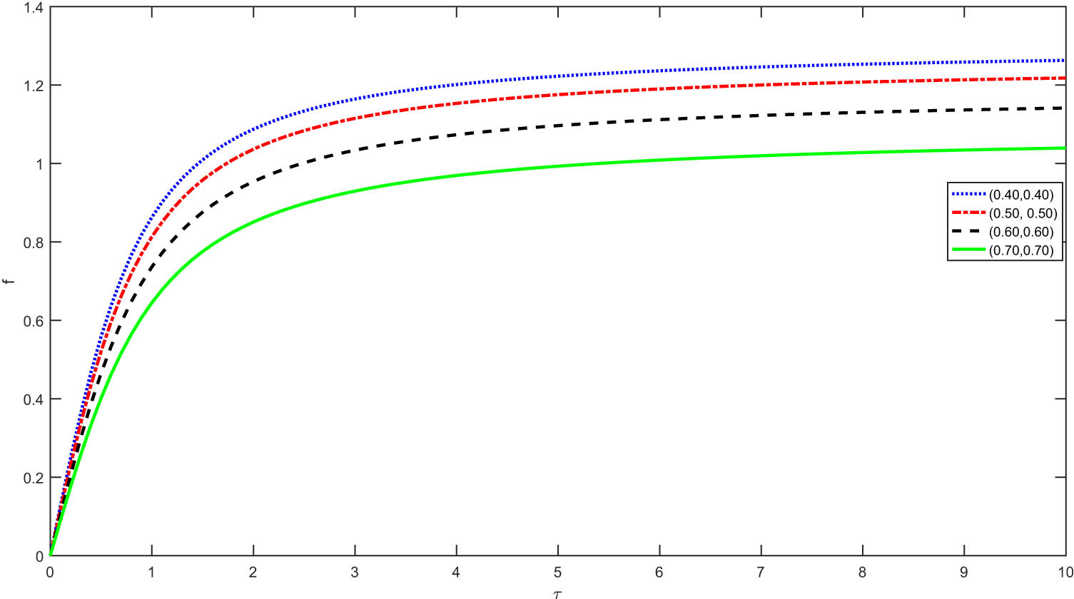
Graphical presentation of numerical solution of Example 1 with respect to different fractal–fractional orders.

In Figure 3, we take larger values for fractal orders corresponding to various fractional order values to understand the effect of fractal dimension.

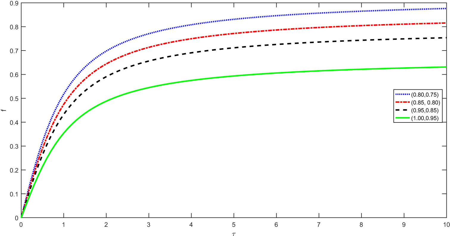
$Figure 3 Graphical presentation of numerical solution of Example 1 with respect to different fractal–fractional orders.$

Figure 3

Graphical presentation of numerical solution of Example 1 with respect to different fractal–fractional orders.

From Figures 1–3, we see that fractal order has a significant impact on the dynamics of the considered problem. For larger fractal dimension, the dispersion between the curves is more than for small fractal order.

Example 2

Consider the given problem:

(18) D τ η , ζ 0 F F f ( τ ) 500 + ∣ f ( τ ) ∣ 3 = cos ( τ ) + ∣ f ( τ ) ∣ τ 2 + 500 , τ ∈ [ 0 , 1 ] , η , ζ ∈ ( 0 , 1 ] , f ( 0 ) = 0 .

It is easy to verify that Conditions A 1 and A 2 hold. Also, the requirement of Theorem 3.1 holds; therefore, Problem (2) has a solution. Furthermore, using different fractal–fractional order, we present the solution graphically using our numerical scheme in Figures 4 and 5 for b = 1 .

$Figure 4 Graphical presentation of numerical solution of Example 2 with respect to different fractal–fractional orders.$

Figure 4

Graphical presentation of numerical solution of Example 2 with respect to different fractal–fractional orders.

$Figure 5 Graphical presentation of numerical solution of Example 2 with respect to different fractal–fractional orders.$

Figure 5

Graphical presentation of numerical solution of Example 2 with respect to different fractal–fractional orders.

In Figure 6, we take larger values for fractal order corresponding to various fractional order values to understand the effect of fractal dimension.

$Figure 6 Graphical presentation of numerical solution of Example 2 with respect to different fractal–fractional orders.$

Figure 6

Graphical presentation of numerical solution of Example 2 with respect to different fractal–fractional orders.

Example 3

Consider the given problem with tangent function:

(19) D τ η , ζ 0 F F f ( τ ) 100 + ∣ f ( τ ) ∣ 2 = tan ( τ ) + ∣ f ( τ ) ∣ 4 exp ( τ ) + 100 , τ ∈ [ 0 , 1 ] , η , ζ ∈ ( 0 , 1 ] , f ( 0 ) = 0 .

We present the numerical solution graphically for different fractals and fractional orders in Figures 7 and 8.

$Figure 7 Graphical presentation of numerical solution of Example 3 with respect to different fractal–fractional orders.$

Figure 7

Graphical presentation of numerical solution of Example 3 with respect to different fractal–fractional orders.

$Figure 8 Graphical presentation of numerical solution of Example 3 with respect to different fractal–fractional orders.$

Figure 8

Graphical presentation of numerical solution of Example 3 with respect to different fractal–fractional orders.

In Figure 9, we take larger values for fractal order corresponding to various fractional order values to understand the effect of fractals dimension.

$Figure 9 Graphical presentation of numerical solution of Example 3 with respect to different fractal–fractional orders.$

Figure 9

Graphical presentation of numerical solution of Example 3 with respect to different fractal–fractional orders.

In Figures 7–9, we demonstrated graphically the approximate solution of Problem (3) for taking different values of fractals and fractional orders. The effect of fractal dimension has been demonstrated in the mentioned figures.

5 Conclusion

Researchers have extensively studied hybrid nonlinear problems of ordinary as well as fractional order. They established the existence theory on using fixed point theorems and studied some comparative results. But the said problems were very rarely studied for numerical solutions using some numerical tools. Also, the newly developed fractal–fractional calculus concepts have not been used to investigate the mentioned area of hybrid nonlinear problems. Therefore, it was recommended to investigate the mentioned problems under fractal–fractional derivatives using hybrid fixed point theorems. Also, a sophisticated numerical method is required to studied the mentioned problems for their numerical solutions because the said problems are nonlinear and it is very difficult to compute the exact or analytical solution. On the other hand, many biological problems can be modeled using HDEs. Therefore, keeping in mind the required need, a class of hybrid nonlinear FFDEs has been studied in this research work. For the mentioned problem, we have designed some sufficient conditions under which the aforesaid problem has exactly a solution. The tool we utilized for to obtain the fundamental results was based on hybrid fixed point theorem for the product of two operators. Sufficient conditions have established for the UH stability to the proposed problem. Moreover, such problems have significant uses in engineering and dynamical fields, and we have derived a numerical scheme based on Euler method for FFDEs. The said numerical scheme has been demonstrated by testing three pertinent examples with graphical illustrations using various fractals and fractional orders. In the future, the said algorithm and analysis will be exercised for more generalized complex hybrid dynamical systems with FFDEs. Also, in the future, the said analysis can be extended to hybrid mathematical models biological tissues using fractal–fractional calculus. The said area will open new doors of research.

kshah@psu.edu.sa

Acknowledgement

Authors are thankful to Prince Sultan University for article processing charges and support through the Theoretical and Applied Sciences Lab.

Funding information: This research is supported by Prince Sultan University through the research lab Theoretical and Applied Sciences (TAS).
Author contributions: Shafiullah wrote the draft. Kamal Shah included the numerical part. Muhammad Sarwar updated the theoretical part. Thabet Abdeljawad has edited and updated the final version.
Conflict of interest: There exists no competing interest regarding this manuscript.
Data availability statement: No data was used during this research work.

References

[1] Machado JT, Kiryakova V, Mainardi F. Recent history of fractional calculus. Commun Nonli Sci Numer Simul. 2011;16(3):1140–53. 10.1016/j.cnsns.2010.05.027Search in Google Scholar

[2] Sabatier JATMJ, Agrawal OP, Machado JT. Advances in fractional calculus. (Vol. 4, No. 9). Dordrecht, Germany: Springer; 2007. 10.1007/978-1-4020-6042-7Search in Google Scholar

[3] Baleanu D, Diethelm K, Scalas E, Trujillo JJ. Fractional calculus: models and numerical methods. Vol. 3. Singapore: World Scientific; 2012. 10.1142/9789814355216Search in Google Scholar

[4] Kilbas AA, Srivastava HM, Trujillo JJ. Theory and applications of fractional differential equations. Vol. 204. Amsterdam: Elsevier; 2006. Search in Google Scholar

[5] Rahimy M. Applications of fractional differential equations. Appl Math Sci. 2010;4(50):2453–61. Search in Google Scholar

[6] Magin RL. Fractional calculus models of complex dynamics in biological tissues. Comput Math Appl. 2010;59(5):1586–93. 10.1016/j.camwa.2009.08.039Search in Google Scholar

[7] Jacob JS, Priya JH, Karthika A. Applications of fractional calculus in science and engineering. J Crit Rev. 2020;7(13):4385–94. Search in Google Scholar

[8] Dhage BC, Lakshmikantham V. Basic results on hybrid differential equations. Nonlinear Anal: Hybrid Syst. 2010;4(3):414–24. 10.1016/j.nahs.2009.10.005Search in Google Scholar

[9] Jarad F, Abdeljawad T. Generalized fractional derivatives and Laplace transform. Discret Contin Dyn Syst Ser. 2020;13:709–22. 10.3934/dcdss.2020039Search in Google Scholar

[10] Ahmad B, Ntouyas SK. Initial-value problems for hybrid Hadamard fractional differential equations. Electron J Differ Equ. 2014;2014:1–8. 10.1186/1687-1847-2014-199Search in Google Scholar

[11] Abbas MI, Ragusa MA. On the hybrid fractional differential equations with fractional proportional derivatives of a function with respect to a certain function. Symmetry. 2021;13(2):264. 10.3390/sym13020264Search in Google Scholar

[12] Gentilini C, Nascimbene R, Ubertini F. Towards an alternative approach to geometrical modelling of shell surfaces using a parametric representation. Proceedings Second MIT Conference on Computational Fluid and Solid Mechanics; 2003 Jun 17-20; Cambridge (MA), USA. Elsevier Science, 2003. p. 288–91. 10.1016/B978-008044046-0.50072-5Search in Google Scholar

[13] Lovadina C, Nascimbene R, Perugia I, Venini P. Mixed methods for interface problems. In: Bathe KJ, editor. Computational Fluid and Solid Mechanics; 2003 Jun 17–20; Cambridge (MA), USA. Elsevier Science, 2003, Elsevier Science Ltd; 2003. p. 2053–6. 10.1016/B978-008044046-0.50503-0Search in Google Scholar

[14] Norouzi M, Davoodi M, Anwar Bég O, Shamshuddin MD. Theoretical study of Oldroyd-B visco-elastic fluid flow through curved pipes with slip effects in polymer flow processing. Int J Appl Comput Math. 2018;4:1–22. 10.1007/s40819-018-0541-7Search in Google Scholar

[15] Shamshuddin M, Mishra SR, Beg OA, Kadir A. Adomian decomposition method simulation of Von Kármán swirling bioconvection nanofluid flow. J Central South Univ. 2019;26(10):2797–813. 10.1007/s11771-019-4214-4Search in Google Scholar

[16] Atangana A. Fractal-fractional differentiation and integration: connecting fractal calculus and fractional calculus to predict complex system. Chaos Solitons Fractals. 2017;102:396–406. 10.1016/j.chaos.2017.04.027Search in Google Scholar

[17] Khan ZA, Shah K, Abdalla B, Abdeljawad T. A numerical study of complex dynamics of a chemostat model under fractal-fractional derivative. Fractals. 2023;31(8):2340181. 10.1142/S0218348X23401813Search in Google Scholar

[18] Khan H, Alzabut J, Shah A, He ZY, Etemad S, Rezapour S, et al. On fractal-fractional waterborne disease model: A study on theoretical and numerical aspects of solutions via simulations. Fractals. 2023;31(4):2340055. 10.1142/S0218348X23400558Search in Google Scholar

[19] Imran MA. Application of fractal–fractional derivative of power law kernel Dxα,β0FFC to MHD viscous fluid flow between two plates. Chaos Solitons Fractals. 2020;134:109691. 10.1016/j.chaos.2020.109691Search in Google Scholar

[20] Atangana A, Qureshi S. Modeling attractors of chaotic dynamical systems with fractal-fractional operators. Chaos Solitons Fractals. 2019;123:320–37. 10.1016/j.chaos.2019.04.020Search in Google Scholar

[21] Shah K, Sinan M, Abdeljawad T, El-Shorbagy MA, Abdalla B, Abualrub MS. A detailed study of a fractal-fractional transmission dynamical model of viral infectious disease with vaccination. Complexity. 2022;2022:21. 10.1155/2022/7236824Search in Google Scholar

[22] Dhage BC. A nonlinear alternative in Banach algebras with applications to functional differential equations. Nonlinear Funct Anal Appl. 2004;8:563–75. Search in Google Scholar

[23] Dhage BC. Fixed point theorems in ordered Banach algebras and applications J Panam Math. 1999;9:93–102. Search in Google Scholar

[24] Baleanu D, Hasib Khan, Jafari H, Khan RA, Alipouri M. On existence results for solutions of coupled system of Hybrid boundary value problems with Hybrid conditions. Adv Differ Equ. 2015;318:1–1410.1186/s13662-015-0651-zSearch in Google Scholar

[25] Owolabi KM, Dutta H. Modelling and analysis of predation system with nonlocal and nonsingular operator. In: Dutta H, editor. Mathematical modelling in health, social and applied sciences. Singapore: Springer; 2020. p. 261–82. 10.1007/978-981-15-2286-4_8Search in Google Scholar

[26] Venini P, Nascimbene R. A new fixed-point algorithm for hardening plasticity based on non-linear mixed variational inequalities. Int J Numer Method Eng. 2003;57(1):83–102. 10.1002/nme.672Search in Google Scholar

[27] Ben Amara K, Berenguer MI, Jeribi A. Approximation of the fixed point of the product of two operators in Banach algebras with applications to some functional equations. Mathematics. 2022;10(22):4179. 10.3390/math10224179Search in Google Scholar

[28] Diethelm K. The analysis of fractional differential equations. Berlin, Germany: Springer; 2010. 10.1007/978-3-642-14574-2Search in Google Scholar

[29] Djebali S, Sahnoun Z. Nonlinear alternatives of Schauder and Krasnoselaskii types with applications to Hammerstein integral equations in L1-spaces. J Differ Equ. 2020;249:2061–75. 10.1016/j.jde.2010.07.013Search in Google Scholar

[30] Borelli C, Forti GL. On a general Hyers-Ulam stability result. Int J Math Math Sci. 1995;18:229–36. 10.1155/S0161171295000287Search in Google Scholar

[31] Khan N, Ahmad Z, Shah J, Murtaza S, Albalwi MD, Ahmad H, et al. Dynamics of chaotic system based on circuit design with Ulam stability through fractal-fractional derivative with power law kernel. Sci Rep. 2023;13(1):5043. 10.1038/s41598-023-32099-1Search in Google Scholar PubMed PubMed Central

[32] Khan MA, Atangana A. Numerical methods for fractal-fractional differential equations and engineering: simulations and modeling. New York (NY), USA: CRC Press; 2023. 10.1201/9781003359258Search in Google Scholar

Received: 2023-09-06

Revised: 2023-12-11

Accepted: 2023-12-30

Published Online: 2024-03-14

This work is licensed under the Creative Commons Attribution 4.0 International License.

Articles in the same Issue

https://doi.org/10.1515/nleng-2022-0372

Keywords for this article

fractals and fractional calculus; hybrid problem; existence theory; numerical results

Creative Commons

BY 4.0