Existence of positive periodic solutions for first-order nonlinear differential equations with multiple time-varying delays
-
Xiaoling Han


Abstract
This study elucidates the sufficient conditions for the first-order nonlinear differential equations with periodic coefficients and time-varying delays to have positive periodic solutions. Our results are proved using the Krasnosel’skii fixed point theorem. In this article, we have identified two sets
1 Introduction
Consider the first-order nonlinear equation
where
We assume that
(H1)
(H2)
(H3)
Equation (1.1) is a delay differential equation. Delay differential equations are mainly used to describe dynamic systems that rely on current and past historical states. The time-delay phenomenon is widely used in the fields of population dynamics [1,2, 3,4] and infectious diseases [5,6]. Scholars have shown that delay differential equations can more accurately reflect the changing laws of objective things than differential equations without time delay. In the past few decades, delay differential equations have received the attention of many scholars and achieved certain results.
For equation (1.1), when the nonlinear term
where
where
When the nonlinear term
where
In recent years, many authors have studied the existence of positive
Here, we introduce the notations required to describe our main results. For each
Define
Let
where
In this article, we also assume that (H4) holds:
(H4)
For simplicity, we refer to points belonging to
2 Auxiliary lemmas and preparations
For convenience, in this section, we would like to introduce some notations, definitions, lemmas, and assumptions which are used in what follows.
Definition 1
[25] Let
Definition 2
[25] An operator
The following is the well-known Krasnoselskii’s fixed point theorem in a cone.
Lemma 1
[25] Let M be a Banach space, and let
be a completely continuous operator such that
Let
be the Banach space of
Define a subset in
It is easy to see that
Lemma 2
The positive
where
Proof
“Only if” part: Let
which is equivalent to
The integration from
By the periodic properties, we obtain that
Thus,
for
“If” part: Take the derivative of (2.1) with respect to
Thus, the proof of Lemma 2 is complete.□
Define a functional
It is clear that
and
Hence, when
Moreover,
Define an operator
The operator
Lemma 3
The operator K defined by (2.3) maps P into P.
Proof
Any element
This means that
and
Form (2.4) and (2.5), we see that
Hence,
The proof of Lemma 3 is complete.□
Lemma 4
The operator
Proof
We need to verify the following two points:
that is,
Therefore, operator
Point (ii): For any
where
Therefore,
On the other hand, let
We can write
This immediately implies that
Therefore, for any
which implies that the operator
3 Simple conditions to ensure the existence of
∇
-point and
Δ
-point
We can prove that (1.1) has sufficient conditions for
If function
then we can find a sufficiently small number
Hence, we see that
For
If for given
Hence, we see that
4 Main results
Theorem 1
Under conditions (H1)–(H3), if there exist a
Proof
To apply Lemma 1, we have to only find open bounded subsets
and
respectively. Any
Any
By (2.2) and (4.1), we obtain
for
Any
By (2.2) and (4.2), we obtain
for
Thus, we have confirmed that assumption (ii) of Lemma 1 is satisfied in the case
Then,
Theorem 2
If
Proof
From Lemma 4, we know that
According to condition
5 Necessary condition
For convenience, let us make an assumption:
where
Theorem 3
Assume that (H1)–(H4) hold and that
for all t. Then every positive solution of equation (1.1) tends to zero as
Proof
Let
Integrating the above from
From (3.1) and (5.1),
Let
Case 1. When
This contradiction shows that Case 1 is impossible.
Case 2. When
Let
Again let
Case 3. When
From (1.1) and (3.1), we have
Transforming the above formula, we have
Choose
From (5.4) and (5.5), we have
Set
which is a contradiction. So we have that
From Theorem 3, we have the following results immediately.
Corollary 1
Let (H1)–(H4) and (5.1) hold. Then equation (1.1) has no positive
Corollary 2
Let (H1)–(H4) hold, and let
6 Example and numerical simulation
In this section, we give an example to illustrate the correctness of our main results.
Example 1
Consider the delayed periodic Nicholson’s blowflies models with a time-varying delay:
Proof
Note that
Then
Thus,
According to the definition of sets
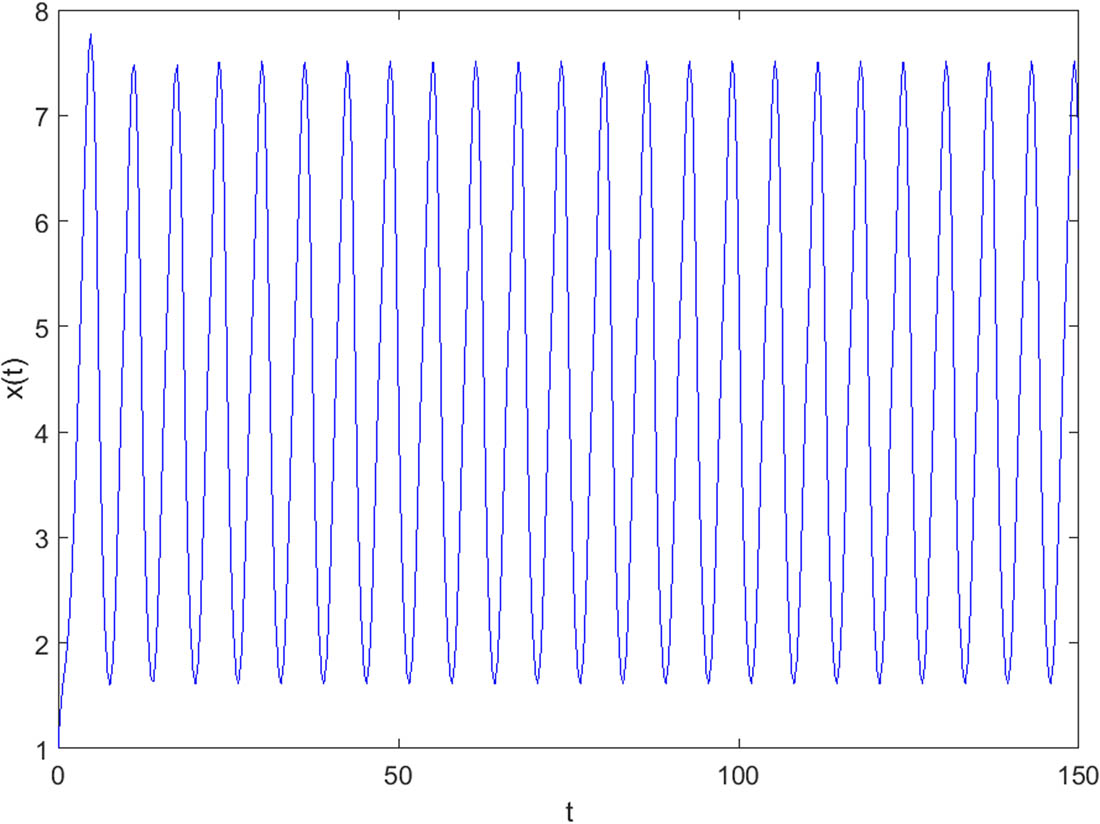
Numerical solution
Example 2
Consider the delayed periodic Nicholson’s blowflies models with time delay:
Proof
Let
Then, we have
Therefore, from Theorem 3, every positive solution of equation (6.2) tends to zero as

Numerical solution
7 Conclusion
In this work, we used Ascoli-Arzela and Krasnosel’skii fixed point theorems and some useful properties of Green’s function to establish the existence of at least one positive periodic solution for our equation. In biology, equation (1.1) can be used to describe the relevant dynamic behavior of different single species, such as Nicholson’s blowflies model and hematopoiesis model. The research work of this article enriches and supplements the findings in the literature and differ from those of [7,13,14,20] in two aspects.
First, when
Second, we prove the existence, uniqueness, and oscillations of the period solutions of equation (1.1) and give the relationship between birth rate, death and harvesting rate when the periodic solution tends to zero.
-
Funding information: This work was supported by NNSF of China (No. 12161079) and Natural Science Foundation of Gansu Province (No. 20JR10RA086).
-
Conflict of interest: The authors state no conflict of interest.
References
[1] J. Cushing, Integro-differential Equations and Delay Models in Population Dynamics, Springer-Verlag, New York, 1977. 10.1007/978-3-642-93073-7Search in Google Scholar
[2] Y. Kuang, Delay Differential Equations with Applications in Population Dynamics, Academic Press, New York, 1993. Search in Google Scholar
[3] H. Freedman and K. Gopalsamy, Global stability in time-delayed single-species dynamics, Bull. Math. Biol. 48 (1986), no. 5, 485–492, https://doi.org/10.1007/BF02462319. Search in Google Scholar PubMed
[4] S. Ruan, Delay Differential Equations in Single Species Dynamics, Springer, Dordrech, 2006. 10.1007/1-4020-3647-7_11Search in Google Scholar
[5] F. Brauer and C. Castillo-Chavez, Mathematical Models in Population Biology and Epidemiology, Springer, New York, 2001. 10.1007/978-1-4757-3516-1Search in Google Scholar
[6] R. Culshaw and S. Ruan, A Delay-Differential Equation Model of HIV Infection of CD4(+) T-Cells, Math. Biosci. 165 (2000), no. 1, 27–39, DOI: https://doi.org/10.1016/S0025-5564(00)00006-7. 10.1016/S0025-5564(00)00006-7Search in Google Scholar
[7] M. Gurney, S. Blythe, and R. Nisbee, Nicholson’s Blowflies Revisited, Nature 287 (1980), 17–21, DOI: https://doi.org/10.1038/287017a0. 10.1038/287017a0Search in Google Scholar
[8] A. Bouakkaz and R. Khemis, Positive periodic solutions for revisited Nicholson’s blowflies equation with iterative harvesting term, J. Math. Anal. Appl. 494 (2021), no. 12, 124663, https://doi.org/10.1016/j.jmaa.2020.124663. Search in Google Scholar
[9] C. Xu, M. Liao, P. Li, Q. Xiao, and S. Yuan, A new method to investigate almost periodic solutions for an Nicholson’s blowflies model with time-varying delays and a linear harvesting term, Math. Biosci. Eng. 16 (2019), no. 5, 3830–3840, https://doi.org/10.3934/mbe.2019189. Search in Google Scholar PubMed
[10] J. Sugie, Y. Yan, and M. Qu, Effect of decimation on positive periodic solutions of discrete generalized Nicholson’s blowflies models with multiple time-varying delays, Commun. Nonlinear Sci. Numer. Simul. 97 (2021), 105731, DOI: https://doi.org/10.1016/j.cnsns.2021.105731. 10.1016/j.cnsns.2021.105731Search in Google Scholar
[11] L. Duan and L. Huang, Pseudo almost periodic dynamics of delay Nicholson’s blowflies model with a linear harvesting term, Math. Methods Appl. Sci. 38 (2015), no. 6, 1178–1189, https://doi.org/10.1002/mma.3138. Search in Google Scholar
[12] F. Long, Positive almost periodic solution for a class of Nicholson’s blowflies model with a linear harvesting term, Nonlinear Anal. Real World Appl. 13 (2012), no. 2, 686–693, https://doi.org/10.1016/j.nonrwa.2011.08.009. Search in Google Scholar
[13] J. Li and C. Du, Existence of positive periodic solutions for a generalized Nicholson’s blowflies model, J. Comput. Appl. Math. 221 (2008), no. 1, 226–233, https://doi.org/10.1016/j.cam.2007.10.049. Search in Google Scholar
[14] M. Mackey and L. Glass, Oscillation and chaos in physiological control system, Science 197 (1977), no. 4300, 287–289, https://doi.org/10.1126/science.267326. Search in Google Scholar PubMed
[15] B. Liu, New results on the positive almost periodic solutions for a model of hematopoiesis, Nonlinear Anal. Real World Appl. 17 (2014), 252–264, https://doi.org/10.1016/j.nonrwa.2013.12.003. Search in Google Scholar
[16] Y. Yan and J. Sugie, Existence regions of positive periodic solutions for a discrete hematopoiesis model with unimodal production functions, Appl. Math. Model. 68 (2019), 152–168, https://doi.org/10.1016/j.apm.2018.11.003. Search in Google Scholar
[17] P. Amster and C. Rocio, Existence and multiplicity of periodic solutions for a generalized hematopoiesis model, J. Appl. Math. Comput. 55 (2017), 591–607, https://doi.org/10.1007/s12190-016-1051-6. Search in Google Scholar
[18] H. Fredj and F. Chèif, Positive pseudo almost periodic solutions to a class of hematopoiesis model: Oscillations and dynamics, J. Appl. Math. Comput. 63 (2020), 479–500, https://doi.org/10.1007/s12190-020-01326-7. Search in Google Scholar
[19] R. Balderrama, New results on the almost periodic solutions for a model of hematopoiesis with an oscillatory circulation loss rate, J. Fixed Point Theory Appl. 22 (2020), no. 42, 1–18, https://doi.org/10.1007/s11784-020-00776-7. Search in Google Scholar
[20] G. Liu, J. Yan, and F. Zhang, Existence and global attractivity of unique positive periodic solution for a model of hematopoiesis, J. Math. Anal. Appl. 334 (2007), no. 1, 157–171, https://doi.org/10.1016/j.jmaa.2006.12.015. Search in Google Scholar
[21] W. Zhao, C. Zhu, and H. Zhu, On positive periodic solution for the delay Nicholson’s Blowflies model with a harvesting term, Appl. Math. Model. 36 (2012), no. 7, 3335–3340, https://doi.org/10.1016/j.apm.2011.10.011. Search in Google Scholar
[22] G. Liu, A. Zhao, and J. Yan, Existence and global attractivity of unique positive periodic solution for a Lasota-Wazewska model, Nonlinear Anal. 64 (2006), no. 8, 1737–1746, https://doi.org/10.1016/j.na.2005.07.022. Search in Google Scholar
[23] C. Xu, M. Liao, P. Li, Z. Liu, and S. Yuan, New results on pseudo almost periodic solutions of quaternion-valued fuzzy cellular neural networks with delays, Fuzzy Sets Systems 411 (2021), no. 2, 25–47, DOI: https://doi.org/10.1016/j.fss.2020.03.016. 10.1016/j.fss.2020.03.016Search in Google Scholar
[24] C. Xu, Z. Liu, L. Yao, and C. Aouiti, Further exploration on bifurcation of fractional-order six-neuron bi-directional associative memory neural networks with multi-delays, Appl. Math. Comput. 410 (2021), 126458, DOI: https://doi.org/10.1016/j.amc.2021.126458. 10.1016/j.amc.2021.126458Search in Google Scholar
[25] D. Guo, Nonlinear Functional Analysis, Shandong Science and Technology Press, Jinan, 2001. Search in Google Scholar
© 2022 Xiaoling Han and Ceyu Lei, published by De Gruyter
This work is licensed under the Creative Commons Attribution 4.0 International License.
Articles in the same Issue
- Regular Articles
- A random von Neumann theorem for uniformly distributed sequences of partitions
- Note on structural properties of graphs
- Mean-field formulation for mean-variance asset-liability management with cash flow under an uncertain exit time
- The family of random attractors for nonautonomous stochastic higher-order Kirchhoff equations with variable coefficients
- The intersection graph of graded submodules of a graded module
- Isoperimetric and Brunn-Minkowski inequalities for the (p, q)-mixed geominimal surface areas
- On second-order fuzzy discrete population model
- On certain functional equation in prime rings
- General complex Lp projection bodies and complex Lp mixed projection bodies
- Some results on the total proper k-connection number
- The stability with general decay rate of hybrid stochastic fractional differential equations driven by Lévy noise with impulsive effects
- Well posedness of magnetohydrodynamic equations in 3D mixed-norm Lebesgue space
- Strong convergence of a self-adaptive inertial Tseng's extragradient method for pseudomonotone variational inequalities and fixed point problems
- Generic uniqueness of saddle point for two-person zero-sum differential games
- Relational representations of algebraic lattices and their applications
- Explicit construction of mock modular forms from weakly holomorphic Hecke eigenforms
- The equivalent condition of G-asymptotic tracking property and G-Lipschitz tracking property
- Arithmetic convolution sums derived from eta quotients related to divisors of 6
- Dynamical behaviors of a k-order fuzzy difference equation
- The transfer ideal under the action of orthogonal group in modular case
- The multinomial convolution sum of a generalized divisor function
- Extensions of Gronwall-Bellman type integral inequalities with two independent variables
- Unicity of meromorphic functions concerning differences and small functions
- Solutions to problems about potentially Ks,t-bigraphic pair
- Monotonicity of solutions for fractional p-equations with a gradient term
- Data smoothing with applications to edge detection
- An ℋ-tensor-based criteria for testing the positive definiteness of multivariate homogeneous forms
- Characterizations of *-antiderivable mappings on operator algebras
- Initial-boundary value problem of fifth-order Korteweg-de Vries equation posed on half line with nonlinear boundary values
- On a more accurate half-discrete Hilbert-type inequality involving hyperbolic functions
- On split twisted inner derivation triple systems with no restrictions on their 0-root spaces
- Geometry of conformal η-Ricci solitons and conformal η-Ricci almost solitons on paracontact geometry
- Bifurcation and chaos in a discrete predator-prey system of Leslie type with Michaelis-Menten prey harvesting
- A posteriori error estimates of characteristic mixed finite elements for convection-diffusion control problems
- Dynamical analysis of a Lotka Volterra commensalism model with additive Allee effect
- An efficient finite element method based on dimension reduction scheme for a fourth-order Steklov eigenvalue problem
- Connectivity with respect to α-discrete closure operators
- Khasminskii-type theorem for a class of stochastic functional differential equations
- On some new Hermite-Hadamard and Ostrowski type inequalities for s-convex functions in (p, q)-calculus with applications
- New properties for the Ramanujan R-function
- Shooting method in the application of boundary value problems for differential equations with sign-changing weight function
- Ground state solution for some new Kirchhoff-type equations with Hartree-type nonlinearities and critical or supercritical growth
- Existence and uniqueness of solutions for the stochastic Volterra-Levin equation with variable delays
- Ambrosetti-Prodi-type results for a class of difference equations with nonlinearities indefinite in sign
- Research of cooperation strategy of government-enterprise digital transformation based on differential game
- Malmquist-type theorems on some complex differential-difference equations
- Disjoint diskcyclicity of weighted shifts
- Construction of special soliton solutions to the stochastic Riccati equation
- Remarks on the generalized interpolative contractions and some fixed-point theorems with application
- Analysis of a deteriorating system with delayed repair and unreliable repair equipment
- On the critical fractional Schrödinger-Kirchhoff-Poisson equations with electromagnetic fields
- The exact solutions of generalized Davey-Stewartson equations with arbitrary power nonlinearities using the dynamical system and the first integral methods
- Regularity of models associated with Markov jump processes
- Multiplicity solutions for a class of p-Laplacian fractional differential equations via variational methods
- Minimal period problem for second-order Hamiltonian systems with asymptotically linear nonlinearities
- Convergence rate of the modified Levenberg-Marquardt method under Hölderian local error bound
- Non-binary quantum codes from constacyclic codes over 𝔽q[u1, u2,…,uk]/⟨ui3 = ui, uiuj = ujui⟩
- On the general position number of two classes of graphs
- A posteriori regularization method for the two-dimensional inverse heat conduction problem
- Orbital stability and Zhukovskiǐ quasi-stability in impulsive dynamical systems
- Approximations related to the complete p-elliptic integrals
- A note on commutators of strongly singular Calderón-Zygmund operators
- Generalized Munn rings
- Double domination in maximal outerplanar graphs
- Existence and uniqueness of solutions to the norm minimum problem on digraphs
- On the p-integrable trajectories of the nonlinear control system described by the Urysohn-type integral equation
- Robust estimation for varying coefficient partially functional linear regression models based on exponential squared loss function
- Hessian equations of Krylov type on compact Hermitian manifolds
- Class fields generated by coordinates of elliptic curves
- The lattice of (2, 1)-congruences on a left restriction semigroup
- A numerical solution of problem for essentially loaded differential equations with an integro-multipoint condition
- On stochastic accelerated gradient with convergence rate
- Displacement structure of the DMP inverse
- Dependence of eigenvalues of Sturm-Liouville problems on time scales with eigenparameter-dependent boundary conditions
- Existence of positive solutions of discrete third-order three-point BVP with sign-changing Green's function
- Some new fixed point theorems for nonexpansive-type mappings in geodesic spaces
- Generalized 4-connectivity of hierarchical star networks
- Spectra and reticulation of semihoops
- Stein-Weiss inequality for local mixed radial-angular Morrey spaces
- Eigenvalues of transition weight matrix for a family of weighted networks
- A modified Tikhonov regularization for unknown source in space fractional diffusion equation
- Modular forms of half-integral weight on Γ0(4) with few nonvanishing coefficients modulo ℓ
- Some estimates for commutators of bilinear pseudo-differential operators
- Extension of isometries in real Hilbert spaces
- Existence of positive periodic solutions for first-order nonlinear differential equations with multiple time-varying delays
- B-Fredholm elements in primitive C*-algebras
- Unique solvability for an inverse problem of a nonlinear parabolic PDE with nonlocal integral overdetermination condition
- An algebraic semigroup method for discovering maximal frequent itemsets
- Class-preserving Coleman automorphisms of some classes of finite groups
- Exponential stability of traveling waves for a nonlocal dispersal SIR model with delay
- Existence and multiplicity of solutions for second-order Dirichlet problems with nonlinear impulses
- The transitivity of primary conjugacy in regular ω-semigroups
- Stability estimation of some Markov controlled processes
- On nonnil-coherent modules and nonnil-Noetherian modules
- N-Tuples of weighted noncommutative Orlicz space and some geometrical properties
- The dimension-free estimate for the truncated maximal operator
- A human error risk priority number calculation methodology using fuzzy and TOPSIS grey
- Compact mappings and s-mappings at subsets
- The structural properties of the Gompertz-two-parameter-Lindley distribution and associated inference
- A monotone iteration for a nonlinear Euler-Bernoulli beam equation with indefinite weight and Neumann boundary conditions
- Delta waves of the isentropic relativistic Euler system coupled with an advection equation for Chaplygin gas
- Multiplicity and minimality of periodic solutions to fourth-order super-quadratic difference systems
- On the reciprocal sum of the fourth power of Fibonacci numbers
- Averaging principle for two-time-scale stochastic differential equations with correlated noise
- Phragmén-Lindelöf alternative results and structural stability for Brinkman fluid in porous media in a semi-infinite cylinder
- Study on r-truncated degenerate Stirling numbers of the second kind
- On 7-valent symmetric graphs of order 2pq and 11-valent symmetric graphs of order 4pq
- Some new characterizations of finite p-nilpotent groups
- A Billingsley type theorem for Bowen topological entropy of nonautonomous dynamical systems
- F4 and PSp (8, ℂ)-Higgs pairs understood as fixed points of the moduli space of E6-Higgs bundles over a compact Riemann surface
- On modules related to McCoy modules
- On generalized extragradient implicit method for systems of variational inequalities with constraints of variational inclusion and fixed point problems
- Solvability for a nonlocal dispersal model governed by time and space integrals
- Finite groups whose maximal subgroups of even order are MSN-groups
- Symmetric results of a Hénon-type elliptic system with coupled linear part
- On the connection between Sp-almost periodic functions defined on time scales and ℝ
- On a class of Harada rings
- On regular subgroup functors of finite groups
- Fast iterative solutions of Riccati and Lyapunov equations
- Weak measure expansivity of C2 dynamics
- Admissible congruences on type B semigroups
- Generalized fractional Hermite-Hadamard type inclusions for co-ordinated convex interval-valued functions
- Inverse eigenvalue problems for rank one perturbations of the Sturm-Liouville operator
- Data transmission mechanism of vehicle networking based on fuzzy comprehensive evaluation
- Dual uniformities in function spaces over uniform continuity
- Review Article
- On Hahn-Banach theorem and some of its applications
- Rapid Communication
- Discussion of foundation of mathematics and quantum theory
- Special Issue on Boundary Value Problems and their Applications on Biosciences and Engineering (Part II)
- A study of minimax shrinkage estimators dominating the James-Stein estimator under the balanced loss function
- Representations by degenerate Daehee polynomials
- Multilevel MC method for weak approximation of stochastic differential equation with the exact coupling scheme
- Multiple periodic solutions for discrete boundary value problem involving the mean curvature operator
- Special Issue on Evolution Equations, Theory and Applications (Part II)
- Coupled measure of noncompactness and functional integral equations
- Existence results for neutral evolution equations with nonlocal conditions and delay via fractional operator
- Global weak solution of 3D-NSE with exponential damping
- Special Issue on Fractional Problems with Variable-Order or Variable Exponents (Part I)
- Ground state solutions of nonlinear Schrödinger equations involving the fractional p-Laplacian and potential wells
- A class of p1(x, ⋅) & p2(x, ⋅)-fractional Kirchhoff-type problem with variable s(x, ⋅)-order and without the Ambrosetti-Rabinowitz condition in ℝN
- Jensen-type inequalities for m-convex functions
- Special Issue on Problems, Methods and Applications of Nonlinear Analysis (Part III)
- The influence of the noise on the exact solutions of a Kuramoto-Sivashinsky equation
- Basic inequalities for statistical submanifolds in Golden-like statistical manifolds
- Global existence and blow up of the solution for nonlinear Klein-Gordon equation with variable coefficient nonlinear source term
- Hopf bifurcation and Turing instability in a diffusive predator-prey model with hunting cooperation
- Efficient fixed-point iteration for generalized nonexpansive mappings and its stability in Banach spaces