On second-order fuzzy discrete population model
-
Qianhong Zhang
 ,
Miao Ouyang
,
Miao Ouyang

Abstract
This work is concerned with dynamical behavior of a second-order fuzzy discrete population model:
where
1 Introduction
The discrete time population model is the most appropriate mathematical description of life histories of organism. These models are used widely in fisheries and many organisms [1]. The Beverton-Holt model also known as the Skellam equation [2] is one of the classic population model that has been studied
where
In model (1), population is assumed to respond instantly to size variations. But in fact, there is a lag between the variations of external conditions and response of the population to these variations. Therefore, population dynamics is indeed described by delay models. For example, Pielou [6] studied the difference equation with delay:
where
Also the generalization of (2) with many delays
where
The generalization of (2) with infinite memory
where
In fact, the identification of the population dynamics model is usually based on the statistical method, starting from data experimentally obtained and on the choice of some method adapted to the identification. These models, even the classic deterministic approach, are subjected to inaccuracies (fuzzy uncertainty) that can be caused by either the nature of the state variables or by parameters as model coefficients.
In our real life, we have learned to deal with uncertainty. Scientists also accept the fact that uncertainty is a very important factor in most applications. Modeling the real life problems in such cases usually involves vagueness or uncertainty. The concept of fuzzy set and system was introduced by Zadeh [9], and its development has been growing rapidly to various situations of theory and application including fuzzy differential and fuzzy difference equations. It is well known that fuzzy difference equation is a difference equation whose parameters or the state variable are fuzzy numbers, and its solutions are sequences of fuzzy numbers. It has been used to model a dynamical system under possibility uncertainty. Due to the applicability of fuzzy difference equation for the analysis of phenomena where imprecision is inherent, this class of difference equation is a very important topic from theoretical point of view and also its applications. Recently, there has been an increasing interest in the study of fuzzy difference equations [10,11,12, 13,14,15, 16,17,18, 19,20,21, 22,23,24, 25,26,27, 28,29].
Inspired with the previous publication, by virtue of the theory of fuzzy difference equation, in this work, we consider the following discrete population model with fuzzy state variable:
where
The main aim of this work is to study the existence of positive solutions of the population dynamics model (5). Furthermore, according to a generation of division (
2 Preliminary and definitions
First, we provide the following definitions.
Definition 2.1
[30]
The support of
For
Definition 2.2
Fuzzy number (parametric form) [30] A fuzzy number
A crisp (real) number
Definition 2.3
[30] The distance between two arbitrary fuzzy numbers
It is clear that
Definition 2.4
[30] Let
Definition 2.5
(Triangular fuzzy number) [30] A triangular fuzzy number (TFN) denoted by
The
The following proposition is fundamental since it characterizes a fuzzy set through the
Proposition 2.1
[30] If
Then, there is
Definition 2.6
[31] Suppose that
provided that
Remark 2.1
According to [31], in this paper, the fuzzy number is positive, if
Case I. If
Case II. If
The fuzzy analog of the boundedness and persistence (see [22,23]) is as follows:
Definition 2.7
A sequence of positive fuzzy numbers
A sequence of positive fuzzy numbers
A sequence of positive fuzzy numbers
Definition 2.8
Let
3 Main results
3.1 Existence of positive solution of population dynamics model (5)
First, we study the existence of positive solutions of the population dynamics model (5). We need the following lemma.
Lemma 3.1
[30] Let
Theorem 3.1
If
Proof
Suppose that there exists a sequence of fuzzy numbers
It follows from (5), (9), and Lemma 3.1 that
Noting Remark 2.1, one of the following two cases holds:
Case I:
Case II:
If Case I holds true, it follows that for
□
Next, the proof is similar to those of Theorem 3.1 [10]. We omit it.
Remark 3.1
From theoretical point of view, the existence of solution for fuzzy difference equation is very important with initial condition. Therefore, in this sense, the existence of positive fuzzy solution for discrete population dynamics model is of vital importance and practical significance. In fact, according to Theorem 3.1, the positive solution of discrete population dynamics model with fuzzy state is a sequence of positive fuzzy numbers, which can describe the fuzzy uncertainty of the dynamics model.
3.2 Dynamics of discrete population model (5)
To study the dynamical behavior of the positive solutions of the discrete population model (5), according to Definition 2.6, we consider two cases.
First, if Case I holds true, the following lemma is essential to the proof of next theorem.
Lemma 3.2
Consider the difference equation:
where
The system exists a trivial equilibrium point
The system exists a unique positive equilibrium
Every positive solution
Proof
(i) Let
It is clear that the trivial equilibrium point
(ii) The linearized equation associated with (13) at equilibrium expressed as follows:
Since
By virtue of Theorem 1.3.7 in [7], we have that the system is locally asymptotically stable.
On the other hand, it is similar to the proof of Theorem 1 in [32], and we can show that
(iii) Let
and the initial values of (15) are satisfied with
It follows from (13), (15), and (16) that
It is clear that every solution
On the other hand, we consider the family of sequences
Without loss of generality, we take
Let the initial conditions of (19) be positive and satisfy the conditions:
Then, we obtain that
Therefore,
So
Theorem 3.2
Consider the discrete population model (5), where parameters
then the following statements are true.
Every positive solution
Every positive solution
Proof
(i) Since
Let
From which, we get for
(ii) Suppose that there exists a fuzzy number
where
Hence, from (26), we have
Let
Therefore, from (28), we have
This completes the proof of the theorem.□
Second, if Case II holds true, it follows that for
We need the following lemmas.
Lemma 3.3
Consider the system of difference equations:
where
then the following statements are true.
The system exists a trivial equilibrium point
The system exists a unique positive equilibrium point
Proof
(i) The linearized equation of system (30) about
where
The characteristic equation of (32) is expressed as follows:
It follows from (31) that there are two roots of characteristic equation outside the unit disk. So the trivial equilibrium
(ii) The linearized equation of system (30) about
where
Let
Clearly,
It is obtained from (36) that
It is well known that
This implies that the equilibrium
Theorem 3.3
Suppose that parameters A and B of discrete fuzzy population model (5) are positive trivial fuzzy numbers (positive real numbers) and
Then, the following statements are true.
Every positive solution
Every positive solution
Proof
(i) The proof is similar to those of (i) in Theorem 3.2. Let
From which, we obtain for
(ii) Suppose that there exists a positive fuzzy number
From (39), we have
Let
Since
Therefore, from (41), we have
This completes the proof of Theorem 3.3.□
Remark 3.2
In the population dynamical model, the parameters of model are derived from statistic data with vagueness or uncertainty. It corresponds to reality to use fuzzy parameters in the population dynamical model. In contrast with the classic population model, the solution of fuzzy population model is within a range of value (approximate value), which are taken into account fuzzy uncertainties. Furthermore, the global asymptotic behavior of the discrete second-order population model are obtained in fuzzy context.
4 Numerical examples
Example 4.1
Consider the following second-order fuzzy discrete population model:
and we take
From (43), we obtain
From (44), we obtain
Therefore, it follows that
From (42), it results in a coupled system of difference equations with parameter
Therefore,
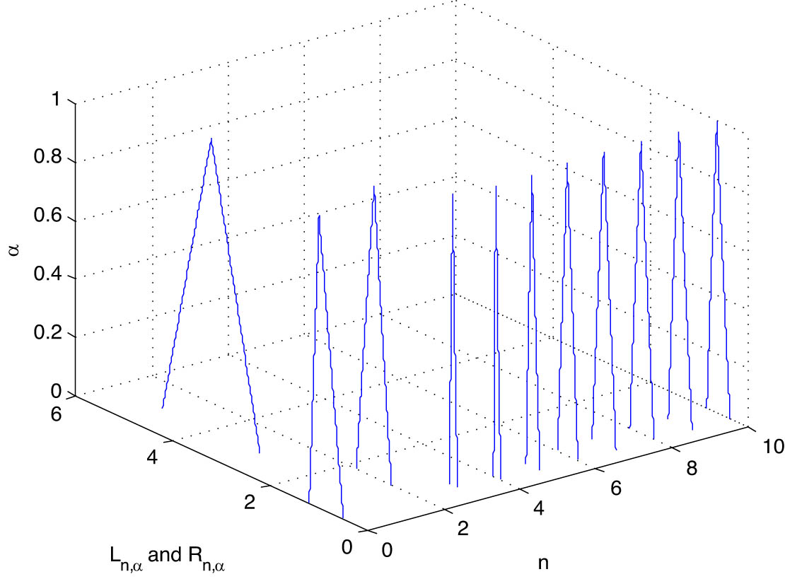
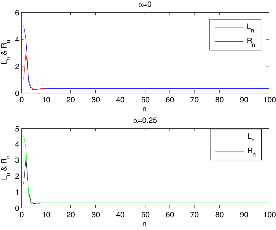
The dynamics of system (42).
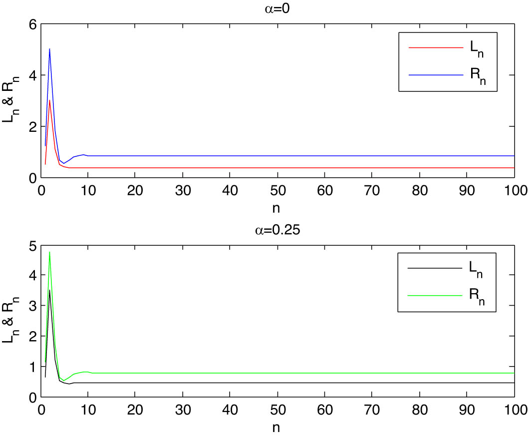
The solution of system (48) at
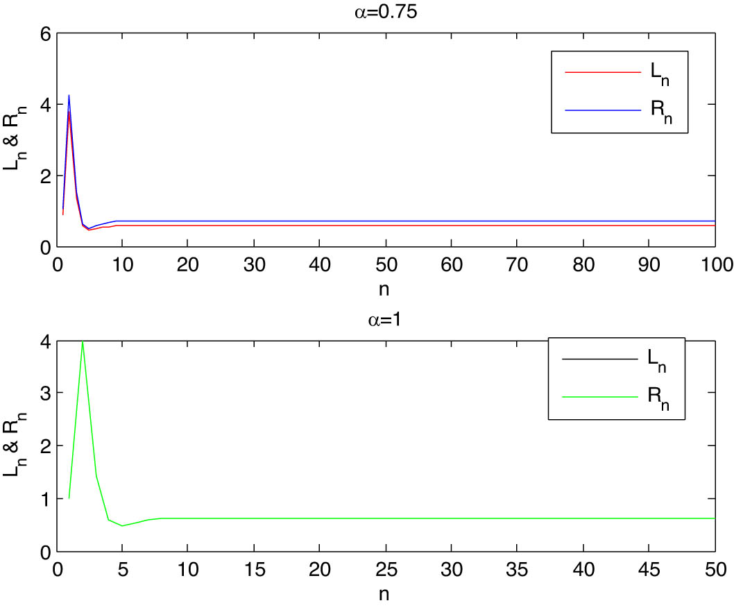
The solution of system (48) at
Example 4.2
Consider the second-order fuzzy discrete population model (42), where
From (48), we obtain
Therefore, it follows that
From (42), it results in a coupled system of difference equation with parameter
It is clear that (38) is satisfied and initial values
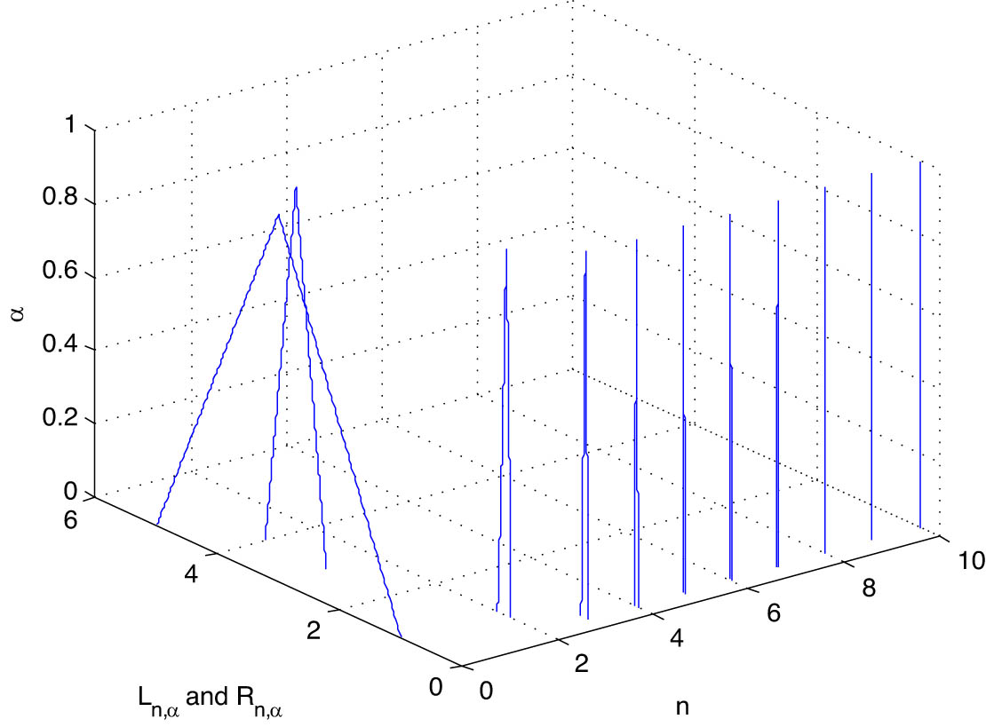
The dynamics of system (42).
The solution of system (48) at
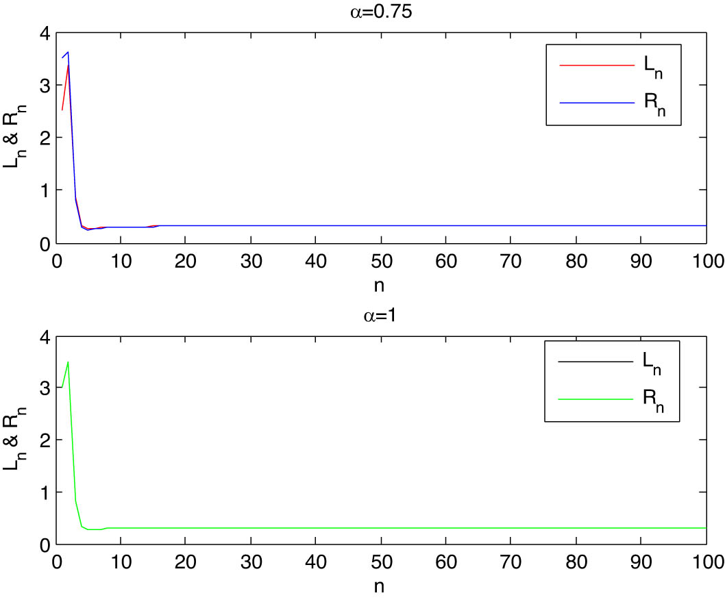
The solution of system (48) at
5 Conclusion
In this work, according to a generalization of division (
Under Case I, the positive solution is bounded and persistent if
Under Case II, the positive solution is bounded and persistent if
-
Funding information: This work was financially supported by the National Natural Science Foundation of China (Grant No. 11761018), Scientific Research Foundation of Guizhou Provincial Department of Science and Technology ([2020]1Y008), and Scientific Climbing Programme of Xiamen University of Technology (XPDKQ20021).
-
Conflict of interest: The authors declare that they have no competing interests.
References
[1] M. Kot, Elements of Mathematical Ecology, Cambridge University Press, New York, 2001, https://doi.org/10.1017/CBO9780511608520.10.1017/CBO9780511608520Search in Google Scholar
[2] R. Beverton and S. Holt, On the Dynamics of Exploited Fish Populations, Springer, Dordrecht, 1993, https://doi.org/10.1007/978-94-011-2106-4. 10.1007/978-94-011-2106-4Search in Google Scholar
[3] M. De la Sen, The generalized Beverton-Holt equation and the control of populations, Appl. Math. Model. 32 (2008), no. 11, 2312–2328, https://doi.org/10.1016/j.apm.2007.09.007. Search in Google Scholar
[4] M. De la Sen and S. Alonso-Quesada Control issues for the Beverton-Holt equation in ecology by locally monitoring the environment carrying capacity: Nonadaptive and adaptive cases, Appl. Math. Comput. 215 (2009), no. 7, 2616–2633, https://doi.org/10.1016/j.amc.2009.09.003. Search in Google Scholar
[5] M. Bohner and S. Streipert, Optimal harvesting policy for the Beverton-Holt model, Math. Biosci. Eng. 13 (2016), no. 4, 673–695, https://doi.org/10.3934/mbe.2016014. Search in Google Scholar
[6] E. C. Pielou, Population and Community Ecology, Gordon and Breach, London, 1975, https://doi.org/10.1016/0013-9327(75)90049-X. 10.1016/0013-9327(75)90049-XSearch in Google Scholar
[7] V. L. Kocic and G. Ladas, Global Behavior of Nonlinear Difference Equations of Higher Order with Applications, Kluwer Academic Publishers, Dordrecht, 1993. 10.1007/978-94-017-1703-8Search in Google Scholar
[8] P. Liu and X. Cui, Hyperbolic logistic difference equations with infinitely many delays, Math. Comput. Simulation 52 (2000), no. 3–4, 231–250, https://doi.org/10.1016/S0378-4754(00)00153-1. 10.1016/S0378-4754(00)00153-1Search in Google Scholar
[9] L. A. Zadeh, Fuzzy sets, Inf. Contr. 8 (1965), no. 3, 338–353, https://doi.org/10.1016/S0019-9958(65)90241-X. 10.21236/AD0608981Search in Google Scholar
[10] E. Y. Deeba, A. De Korvin, and E. L. Koh, A fuzzy difference equation with an application, J. Difference Equ. Appl. 2 (1996), no. 4, 365–374, https://doi.org/10.1080/10236199608808071. Search in Google Scholar
[11] E. Y. Deeba and A. De Korvin, Analysis by fuzzy difference equations of a model of CO2 level in the blood, Appl. Math. Lett. 12 (1999), no. 3, 33–40, https://doi.org/10.1016/S0893-9659(98)00168-2. 10.1016/S0893-9659(98)00168-2Search in Google Scholar
[12] G. Papaschinopoulos and B. K. Papadopoulos, On the fuzzy difference equation xn+1=A+B∕xn, Soft Comput. 6 (2002), 456–461, https://doi.org/10.1007/s00500-001-0161-7. Search in Google Scholar
[13] G. Papaschinopoulos and B. K. Papadopoulos, On the fuzzy difference equation xn+1=A+xn∕xn−m, Fuzzy Sets and Systems 129 (2002), no. 1, 73–81, https://doi.org/10.1016/S0165-0114(01)00198-1. 10.1016/S0165-0114(01)00198-1Search in Google Scholar
[14] G. Stefanidou, G. Papaschinopoulos, and C. J. Schinas, On an exponential-type fuzzy difference equation, Adv. Diff. Equ. 2010 (2010), 196920, https://doi.org/10.1155/2010/. Search in Google Scholar
[15] Q. Din, Asymptotic behavior of a second-order fuzzy rational difference equations, J. Discrete Math. 2015 (2015), 524931, https://doi.org/10.1155/2015/524931. Search in Google Scholar
[16] R. Memarbashi and A. Ghasemabadi, Fuzzy difference equations of volterra type, Int. J. Nonlinear Anal. Appl. 4 (2013), no. 1, 74–78, https://doi.org/10.22075/IJNAA.2013.56. Search in Google Scholar
[17] K. A. Chrysafis, B. K. Papadopoulos, and G. Papaschinopoulos, On the fuzzy difference equations of finance, Fuzzy Sets and Systems 159 (2008), no. 24, 3259–3270, https://doi.org/10.1016/j.fss.2008.06.007. Search in Google Scholar
[18] Q. Zhang, L. Yang, and D. Liao, Behaviour of solutions to a fuzzy nonlinear difference equation, Iran. J. Fuzzy Syst. 9 (2012), no. 2, 1–12, https://doi.org/10.22111/ijfs.2012.186. Search in Google Scholar
[19] Q. Zhang, L. Yang, and D. Liao, On first order fuzzy Ricatti difference equation, Inf. Sci. 270 (2014), no. 20, 226–236, https://doi.org/10.1016/j.ins.2014.02.086. Search in Google Scholar
[20] Q. Zhang, J. Liu, and Z. Luo, Dynamical behavior of a third-order rational fuzzy difference equation, Adv. Differ. Equ. 2015 (2015), 108, https://doi.org/10.1186/s13662-015-0438-2. Search in Google Scholar
[21] S. P. Mondal, D. K. Vishwakarma, and A. K. Saha, Solution of second-order linear fuzzy difference equation by Lagrangeas multiplier method, J. Soft Comput. Appl. 2016 (2016), no. 1, 11–27. 10.5899/2016/jsca-00063Search in Google Scholar
[22] Z. Alijani and F. Tchier, On the fuzzy difference equation of higher order, J. Comput. Complex. Appl. 3 (2017), no. 1, 44–49, https://www.researchgate.net/publication/312166491. Search in Google Scholar
[23] A. Khastan, Fuzzy Logistic difference equation, Iran. J. Fuz. Syst. 15 (2018), no. 7, 55–66, https://doi.org/10.22111/ijfs.2018.4281. Search in Google Scholar
[24] C. Wang, X. Su, P. Liu, X. Hu, and R. Li, On the dynamics of a five-order fuzzy difference equation, J. Nonlinear Sci. Appl. 10 (2017), no. 6, 3303–3319, https://doi.org/10.22436/jnsa.010.06.40. Search in Google Scholar
[25] A. Khastan and Z. Alijani, On the new solutions to the fuzzy difference equation xn+1=A+B∕xn, Fuzzy Sets and Systems 358 (2019), no. 1, 64–83, https://doi.org/https://doi.org/10.1016/j.fss.2018.03.014. Search in Google Scholar
[26] A. Khastan, New solutions for first order linear fuzzy difference equations, J. Comput. Appl. Math. 312 (2017), no. 1, 156–166, https://doi.org/10.1016/j.cam.2016.03.004. Search in Google Scholar
[27] C. Wang, J. Li, and L. Jia, Dynamics of a high-order nonlinear fuzzy difference equation, J. Appl. Anal. Comput. 11 (2021), no. 1, 404–421, https://doi.org/https://doi.org/10.11948/20200050. Search in Google Scholar
[28] C. Wang and J. Li, Periodic solution for a max-type fuzzy difference equation, J. Math. 2020 (2020), no. 3, 1–12, https://doi.org/10.1155/2020/3094391. Search in Google Scholar
[29] C. Wang, X. Su, P. Liu, X. Hu, and R. Li, On the dynamics of a five-order fuzzy difference equation, J. Nonlinear Sci. Appl. 10 (2017), no. 6, 3303–3319, https://doi.org/10.22436/jnsa.010.06.40. Search in Google Scholar
[30] D. Dubois and H. Prade, Possibility Theory: An Approach to Computerized Processing of Uncertainty, Plenum Publishing Corporation, New York, 1998, https://doi.org/10.1137/1034034. Search in Google Scholar
[31] L. Stefanini, A generalization of Hukuhara difference and division for interval and fuzzy arithmetic, Fuzzy Sets and Systems 161 (2010), no. 11, 1564–1584, https://doi.org/10.1016/j.fss.2009.06.009. Search in Google Scholar
[32] R. M. Nigmatulin, Global stability of a discrete population dynamics model with two delays, Autom. Remote Control 66 (2005), 1964–1971, https://doi.org/10.1007/s10513-005-0228-5. Search in Google Scholar
© 2022 Qianhong Zhang et al., published by De Gruyter
This work is licensed under the Creative Commons Attribution 4.0 International License.
Articles in the same Issue
- Regular Articles
- A random von Neumann theorem for uniformly distributed sequences of partitions
- Note on structural properties of graphs
- Mean-field formulation for mean-variance asset-liability management with cash flow under an uncertain exit time
- The family of random attractors for nonautonomous stochastic higher-order Kirchhoff equations with variable coefficients
- The intersection graph of graded submodules of a graded module
- Isoperimetric and Brunn-Minkowski inequalities for the (p, q)-mixed geominimal surface areas
- On second-order fuzzy discrete population model
- On certain functional equation in prime rings
- General complex Lp projection bodies and complex Lp mixed projection bodies
- Some results on the total proper k-connection number
- The stability with general decay rate of hybrid stochastic fractional differential equations driven by Lévy noise with impulsive effects
- Well posedness of magnetohydrodynamic equations in 3D mixed-norm Lebesgue space
- Strong convergence of a self-adaptive inertial Tseng's extragradient method for pseudomonotone variational inequalities and fixed point problems
- Generic uniqueness of saddle point for two-person zero-sum differential games
- Relational representations of algebraic lattices and their applications
- Explicit construction of mock modular forms from weakly holomorphic Hecke eigenforms
- The equivalent condition of G-asymptotic tracking property and G-Lipschitz tracking property
- Arithmetic convolution sums derived from eta quotients related to divisors of 6
- Dynamical behaviors of a k-order fuzzy difference equation
- The transfer ideal under the action of orthogonal group in modular case
- The multinomial convolution sum of a generalized divisor function
- Extensions of Gronwall-Bellman type integral inequalities with two independent variables
- Unicity of meromorphic functions concerning differences and small functions
- Solutions to problems about potentially Ks,t-bigraphic pair
- Monotonicity of solutions for fractional p-equations with a gradient term
- Data smoothing with applications to edge detection
- An ℋ-tensor-based criteria for testing the positive definiteness of multivariate homogeneous forms
- Characterizations of *-antiderivable mappings on operator algebras
- Initial-boundary value problem of fifth-order Korteweg-de Vries equation posed on half line with nonlinear boundary values
- On a more accurate half-discrete Hilbert-type inequality involving hyperbolic functions
- On split twisted inner derivation triple systems with no restrictions on their 0-root spaces
- Geometry of conformal η-Ricci solitons and conformal η-Ricci almost solitons on paracontact geometry
- Bifurcation and chaos in a discrete predator-prey system of Leslie type with Michaelis-Menten prey harvesting
- A posteriori error estimates of characteristic mixed finite elements for convection-diffusion control problems
- Dynamical analysis of a Lotka Volterra commensalism model with additive Allee effect
- An efficient finite element method based on dimension reduction scheme for a fourth-order Steklov eigenvalue problem
- Connectivity with respect to α-discrete closure operators
- Khasminskii-type theorem for a class of stochastic functional differential equations
- On some new Hermite-Hadamard and Ostrowski type inequalities for s-convex functions in (p, q)-calculus with applications
- New properties for the Ramanujan R-function
- Shooting method in the application of boundary value problems for differential equations with sign-changing weight function
- Ground state solution for some new Kirchhoff-type equations with Hartree-type nonlinearities and critical or supercritical growth
- Existence and uniqueness of solutions for the stochastic Volterra-Levin equation with variable delays
- Ambrosetti-Prodi-type results for a class of difference equations with nonlinearities indefinite in sign
- Research of cooperation strategy of government-enterprise digital transformation based on differential game
- Malmquist-type theorems on some complex differential-difference equations
- Disjoint diskcyclicity of weighted shifts
- Construction of special soliton solutions to the stochastic Riccati equation
- Remarks on the generalized interpolative contractions and some fixed-point theorems with application
- Analysis of a deteriorating system with delayed repair and unreliable repair equipment
- On the critical fractional Schrödinger-Kirchhoff-Poisson equations with electromagnetic fields
- The exact solutions of generalized Davey-Stewartson equations with arbitrary power nonlinearities using the dynamical system and the first integral methods
- Regularity of models associated with Markov jump processes
- Multiplicity solutions for a class of p-Laplacian fractional differential equations via variational methods
- Minimal period problem for second-order Hamiltonian systems with asymptotically linear nonlinearities
- Convergence rate of the modified Levenberg-Marquardt method under Hölderian local error bound
- Non-binary quantum codes from constacyclic codes over 𝔽q[u1, u2,…,uk]/⟨ui3 = ui, uiuj = ujui⟩
- On the general position number of two classes of graphs
- A posteriori regularization method for the two-dimensional inverse heat conduction problem
- Orbital stability and Zhukovskiǐ quasi-stability in impulsive dynamical systems
- Approximations related to the complete p-elliptic integrals
- A note on commutators of strongly singular Calderón-Zygmund operators
- Generalized Munn rings
- Double domination in maximal outerplanar graphs
- Existence and uniqueness of solutions to the norm minimum problem on digraphs
- On the p-integrable trajectories of the nonlinear control system described by the Urysohn-type integral equation
- Robust estimation for varying coefficient partially functional linear regression models based on exponential squared loss function
- Hessian equations of Krylov type on compact Hermitian manifolds
- Class fields generated by coordinates of elliptic curves
- The lattice of (2, 1)-congruences on a left restriction semigroup
- A numerical solution of problem for essentially loaded differential equations with an integro-multipoint condition
- On stochastic accelerated gradient with convergence rate
- Displacement structure of the DMP inverse
- Dependence of eigenvalues of Sturm-Liouville problems on time scales with eigenparameter-dependent boundary conditions
- Existence of positive solutions of discrete third-order three-point BVP with sign-changing Green's function
- Some new fixed point theorems for nonexpansive-type mappings in geodesic spaces
- Generalized 4-connectivity of hierarchical star networks
- Spectra and reticulation of semihoops
- Stein-Weiss inequality for local mixed radial-angular Morrey spaces
- Eigenvalues of transition weight matrix for a family of weighted networks
- A modified Tikhonov regularization for unknown source in space fractional diffusion equation
- Modular forms of half-integral weight on Γ0(4) with few nonvanishing coefficients modulo ℓ
- Some estimates for commutators of bilinear pseudo-differential operators
- Extension of isometries in real Hilbert spaces
- Existence of positive periodic solutions for first-order nonlinear differential equations with multiple time-varying delays
- B-Fredholm elements in primitive C*-algebras
- Unique solvability for an inverse problem of a nonlinear parabolic PDE with nonlocal integral overdetermination condition
- An algebraic semigroup method for discovering maximal frequent itemsets
- Class-preserving Coleman automorphisms of some classes of finite groups
- Exponential stability of traveling waves for a nonlocal dispersal SIR model with delay
- Existence and multiplicity of solutions for second-order Dirichlet problems with nonlinear impulses
- The transitivity of primary conjugacy in regular ω-semigroups
- Stability estimation of some Markov controlled processes
- On nonnil-coherent modules and nonnil-Noetherian modules
- N-Tuples of weighted noncommutative Orlicz space and some geometrical properties
- The dimension-free estimate for the truncated maximal operator
- A human error risk priority number calculation methodology using fuzzy and TOPSIS grey
- Compact mappings and s-mappings at subsets
- The structural properties of the Gompertz-two-parameter-Lindley distribution and associated inference
- A monotone iteration for a nonlinear Euler-Bernoulli beam equation with indefinite weight and Neumann boundary conditions
- Delta waves of the isentropic relativistic Euler system coupled with an advection equation for Chaplygin gas
- Multiplicity and minimality of periodic solutions to fourth-order super-quadratic difference systems
- On the reciprocal sum of the fourth power of Fibonacci numbers
- Averaging principle for two-time-scale stochastic differential equations with correlated noise
- Phragmén-Lindelöf alternative results and structural stability for Brinkman fluid in porous media in a semi-infinite cylinder
- Study on r-truncated degenerate Stirling numbers of the second kind
- On 7-valent symmetric graphs of order 2pq and 11-valent symmetric graphs of order 4pq
- Some new characterizations of finite p-nilpotent groups
- A Billingsley type theorem for Bowen topological entropy of nonautonomous dynamical systems
- F4 and PSp (8, ℂ)-Higgs pairs understood as fixed points of the moduli space of E6-Higgs bundles over a compact Riemann surface
- On modules related to McCoy modules
- On generalized extragradient implicit method for systems of variational inequalities with constraints of variational inclusion and fixed point problems
- Solvability for a nonlocal dispersal model governed by time and space integrals
- Finite groups whose maximal subgroups of even order are MSN-groups
- Symmetric results of a Hénon-type elliptic system with coupled linear part
- On the connection between Sp-almost periodic functions defined on time scales and ℝ
- On a class of Harada rings
- On regular subgroup functors of finite groups
- Fast iterative solutions of Riccati and Lyapunov equations
- Weak measure expansivity of C2 dynamics
- Admissible congruences on type B semigroups
- Generalized fractional Hermite-Hadamard type inclusions for co-ordinated convex interval-valued functions
- Inverse eigenvalue problems for rank one perturbations of the Sturm-Liouville operator
- Data transmission mechanism of vehicle networking based on fuzzy comprehensive evaluation
- Dual uniformities in function spaces over uniform continuity
- Review Article
- On Hahn-Banach theorem and some of its applications
- Rapid Communication
- Discussion of foundation of mathematics and quantum theory
- Special Issue on Boundary Value Problems and their Applications on Biosciences and Engineering (Part II)
- A study of minimax shrinkage estimators dominating the James-Stein estimator under the balanced loss function
- Representations by degenerate Daehee polynomials
- Multilevel MC method for weak approximation of stochastic differential equation with the exact coupling scheme
- Multiple periodic solutions for discrete boundary value problem involving the mean curvature operator
- Special Issue on Evolution Equations, Theory and Applications (Part II)
- Coupled measure of noncompactness and functional integral equations
- Existence results for neutral evolution equations with nonlocal conditions and delay via fractional operator
- Global weak solution of 3D-NSE with exponential damping
- Special Issue on Fractional Problems with Variable-Order or Variable Exponents (Part I)
- Ground state solutions of nonlinear Schrödinger equations involving the fractional p-Laplacian and potential wells
- A class of p1(x, ⋅) & p2(x, ⋅)-fractional Kirchhoff-type problem with variable s(x, ⋅)-order and without the Ambrosetti-Rabinowitz condition in ℝN
- Jensen-type inequalities for m-convex functions
- Special Issue on Problems, Methods and Applications of Nonlinear Analysis (Part III)
- The influence of the noise on the exact solutions of a Kuramoto-Sivashinsky equation
- Basic inequalities for statistical submanifolds in Golden-like statistical manifolds
- Global existence and blow up of the solution for nonlinear Klein-Gordon equation with variable coefficient nonlinear source term
- Hopf bifurcation and Turing instability in a diffusive predator-prey model with hunting cooperation
- Efficient fixed-point iteration for generalized nonexpansive mappings and its stability in Banach spaces