Fast iterative solutions of Riccati and Lyapunov equations
-


Abstract
In this article, new iterative algorithms for solving the discrete Riccati and Lyapunov equations are derived in the case where the transition matrix is diagonalizable with real eigenvalues. It is shown that the proposed iterative algorithms are faster than the classical ones, even for a small number of iterations.
1 Introduction
The discrete time Riccati equation arises by implementing the discrete time Kalman filter, which is the most famous estimation algorithm associated with time invariant models of the form [1]:
for
In these models,
Kalman filter produces iteratively the state prediction with the associated prediction error covariance as well as the state estimation with the associated estimation error covariance. The equations of the discrete time Kalman filter result in the discrete time Riccati equation:
Riccati equation relates two successive values of the prediction error covariance
It is well known [1] that if the system is asymptotically stable, i.e., all eigenvalues of the transition matrix
This limiting solution satisfies the algebraic Riccati equation (or steady-state Riccati equation):
It is worth to note that inverse of the matrix
The nonsingularity of
where
The limiting solution
In the infinite measurement noise case, the discrete time Lyapunov equation is derived:
with a limiting solution
The importance of the Riccati and Lyapunov equations is undoubtable: the Riccati equation plays a very important role in various problems of stochastic filtering, statistics, ladder networks, and dynamic programming [1,2], and has many applications in the process of obtaining optimal control and determining system stability [3,4]; Lyapunov equations play a very important role in the stability theory of discrete systems [1,5].
Significant bibliography exists concerning iterative as well as noniterative solutions of the Riccati and Lyapunov equations [1,2,6,7,8,9,10,11,12,13]. The existence of the unique solution of the Riccati equation and of the Lyapunov equation requires the knowledge of the eigenvalues of the transition matrix. The classical iterative solution of the Riccati equation implements the iterative Riccati equation (3) or the iterative transformed Riccati equation (6) till the steady-state solution is reached. Similarly, the classical iterative solution of the Lyapunov equation implements the iterative Lyapunov equation (7) till the steady-state solution is reached.
The aim of this article is to study the optimal algorithm for solving the discrete Riccati and Lyapunov equations, in the case where the transition matrix is diagonalizable with real eigenvalues. The required condition appears in various application areas, see the eigenvalues of the transition matrix in the radar tracking system [14], in the eye movement prediction model [15], and in the mobile position tracking model [16,17]; the state and parameter estimation has been derived using a transition matrix, which is a diagonal itself [18]. The novelty of this article concerns the exploitation of the knowledge of the eigenvalues and eigenvectors of the transition matrix, which leads to the development of the new algorithms for iterative solving of the Riccati and Lyapunov equations, which are superior to classical algorithms, since the proposed algorithms are in general faster than the classical ones.
This article is organized as follows: In Section 2, new iterative solutions of the Riccati and Lyapunov equations are derived by the eigenvalues and eigenvectors of the transition matrix. In Section 3, the proposed algorithms are compared to the classical ones with respect to their computational burdens. Section 4 summarizes the conclusions.
2 New iterative solution algorithms for Riccati equation and Lyapunov equation
Recall that the model parameters
In the following, we consider that the
Consider the diagonalization formula of the transition matrix F given by
where
It is worth noting that equation (11) is essential for the derivation of the new iterative algorithms for solving the discrete Riccati and Lyapunov equations, since they use the eigenvalues and eigenvectors of the transition matrix instead of the transition matrix itself, reducing the computations due to the similarity of the matrices
Concerning the Riccati equation, by multiplying the left-hand side of equation (3) by
Setting in the latter equality
arises the modified Riccati equation.
It is important to note that the Riccati equation (3) with parameters
Then, the limiting solution of (15) is
and satisfies the modified algebraic Riccati equation:
It is clear that the solution of the Riccati equation (3) can be computed by the solution of the modified Riccati Equation (15) due to (16) and (12):
Concerning the transformed Riccati equation, by multiplying the left-hand side of equation (6) by
Setting in the latter equality
It is important to note that the transformed Riccati equation (6) with parameters
Then, using (16)
arises the limiting solution of (21), which satisfies the algebraic Riccati equation:
It is clear that the solution of the transformed Riccati equation (6) can be computed by the solution of the Riccati equation (22) due to (16) and (19):
Concerning the Lyapunov equation, by multiplying the left-hand side of (9) by
Setting in the latter equality
arises
It is important to note that the Lyapunov equation (9) with parameters
Then, using (16)
arises the limiting solution of (25), which satisfies the modified algebraic Lyapunov equation:
It is clear that the solution of the Lyapunov equation (9) can be computed by the solution of the modified Lyapunov equation (25) due to (16) and (24):
Table 1 summarizes the classical and the derived iterative algorithms for solving the Riccati and Lyapunov equations.
Riccati and Lyapunov equations iterative solution algorithms
| Equation | Algorithm | |
|---|---|---|
| Riccati equation | Classical | input:
|
| Proposed | input:
|
|
| Transformed Riccati equation | Classical | input:
|
| Proposed | input:
|
|
| Lyapunov equation | Classical | input:
|
| Proposed | input:
|
|
3 Comparison of classical and proposed algorithms
It is established that the proposed iterative algorithms for solving the Riccati and Lyapunov equations have been derived by the classical iterative algorithms. Thus, the classical and the derived algorithms are equivalent with respect to their behavior since they calculate theoretically the same solutions executing the same number of iterations
We are going to compare the classical and the derived algorithms with respect to their calculation burdens. Scalar operations are involved in matrix manipulation operations, which are needed for the implementation of the algorithms. Table 2 summarizes the calculation burdens of needed matrix operations. The computation of the eigenvalues is achieved by solving the characteristic equation using the Newton-Raphson method, Laguerre’s method, Regula-Falsi method or Bernoulli’s method, because each method requires different computations for solving the characteristic equation. In the following, we consider that all the algorithms apply the same method; thus the computation of the eigenvalues has the same calculation burden, which is denoted as
Calculation burdens of matrix operations
| Matrix operation | Matrix dimensions | Calculation burden |
|---|---|---|
|
|
|
|
|
|
|
|
|
|
|
|
|
(1)
|
|
|
|
|
|
|
|
(1)
|
|
|
|
(2)
|
|
|
|
(2)
|
|
|
|
(3)
|
|
|
(1)
(2)
(3) For the general multi-dimensional case, where
Table 3 summarizes the calculation burdens of the classical and the proposed algorithms, for the general multidimensional case, where
Calculation burdens of algorithms
| Equation | Algorithm | Calculation burden |
|---|---|---|
| Riccati equation | Classical |
|
| Proposed |
|
|
| Transformed Riccati equation | Classical |
|
| Proposed |
|
|
| Lyapunov equation | Classical |
|
| Proposed |
|
Concerning the Riccati equation solution algorithms, from Table 3, we can write:
Note that in the case
since
The aforementioned notation leads to the conclusion that the proposed algorithm is faster than the classical algorithm for a small number of iterations, especially when the state and measurement dimensions are large.
Figure 1 depicts the faster algorithm with respect to the state dimension
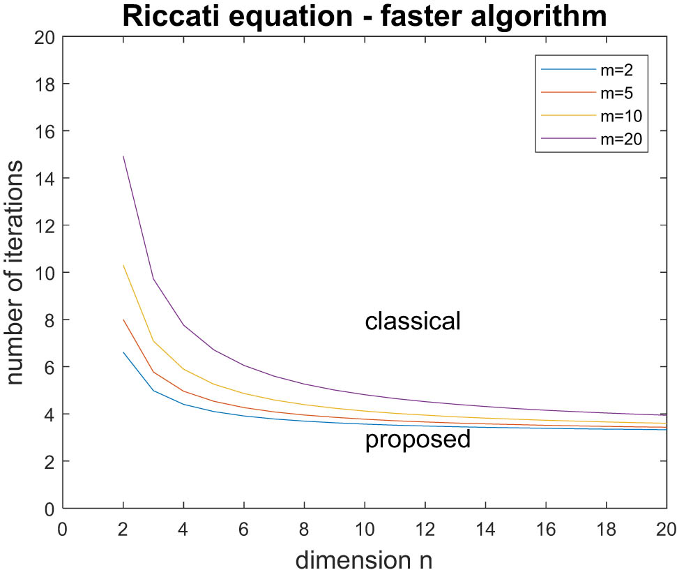
Comparison of the Riccati equation solution algorithms.
Concerning the transformed Riccati equation solution algorithms, from Table 3, we obtain:
Note that in the case
since
The aforementioned notation leads to the conclusion that the proposed algorithm is faster than the classical algorithm for a small number of iterations. In fact, the proposed algorithm is always faster than the classical algorithm, when
Figure 2 depicts the faster algorithm with respect to the state dimension
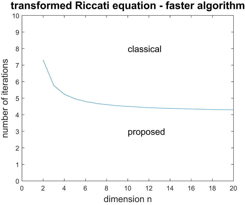
Comparison of transformed Riccati equation solution algorithms.
Concerning the Lyapunov equation solution algorithms, from Table 3, we obtain:
Note that in the case
since
The aforementioned notation leads to the conclusion that the proposed algorithm is faster than the classical algorithm for a small number of iterations. In fact, the proposed algorithm is always faster than the classical algorithm, when
Figure 3 depicts the faster algorithm with respect to the state dimension
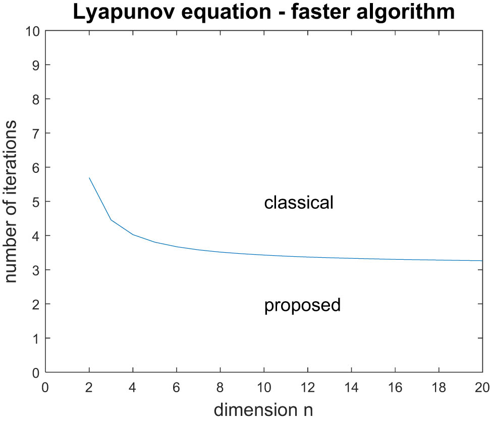
Comparison of Lyapunov equation solution algorithms.
4 Conclusions
Riccati and Lyapunov equations are very important in many fields of science. The existence of their solutions involves the knowledge of the eigenvalues of the transition matrix. We have developed new fast iterative algorithms for solving the Riccati and Lyapunov equations. The proposed algorithms take advantage of the knowledge of the eigenvalues and eigenvectors of the transition matrix. The proposed algorithms hold in the case where the transition matrix is diagonalizable in the form
More specifically,
Concerning the Riccati equation, the proposed solution is faster than the classical one for a small number of iterations, especially when the state and measurement dimensions are large.
Concerning the transformed Riccati equation, the proposed solution is always faster than the classical one when the number of iterations is greater than 7; the proposed algorithm outperforms the classical one when the number of iterations is greater than 4, as the state dimension increases.
Concerning the Lyapunov equation, the proposed solution is always faster than the classical one when the number of iterations is greater than 5; the proposed algorithm outperforms the classical one when the number of iterations is greater than 3, as the state dimension increases.
It is evident that the proposed iterative algorithms outperform the classical ones even for a small number of iterations.
Acknowledgements
The authors thank the anonymous reviewers for their helpful comments.
-
Funding information: The authors state that no funding was involved.
-
Author contributions: The authors applied the SDC approach for the sequence of authors. NA: conceptualization and performed the simulation. MA: performed the formal analysis and prepared the manuscript.
-
Conflict of interest: The authors state no conflict of interest.
-
Data availability statement: All data generated or analyzed during this study are included in this published article.
Appendix
The calculation burdens of the classical and the proposed algorithms for solving the Riccati and Lyapunov equations, for the general multi-dimensional case (where
Riccati equation – classical iterative algorithm
| Initialization | ||
|
|
|
|
| Iteration (
|
||
|
|
|
|
|
|
|
|
|
|
|
|
|
|
|
|
|
|
|
|
|
|
|
|
|
|
|
|
|
|
|
|
|
|
|
|
|
|
|
|
|
|
||
Riccati equation – proposed iterative algorithm
| Initialization | ||
|
|
|
|
|
|
|
|
|
|
|
|
|
|
|
|
|
|
|
|
|
|
|
|
| Iteration (
|
||
|
|
|
|
|
|
|
|
|
|
|
|
|
|
|
|
|
|
|
|
|
|
|
|
|
|
|
|
|
|
|
|
|
|
|
|
|
|
|
|
| Finalization | ||
|
|
|
|
|
|
|
|
|
|
||
Transformed Riccati equation – classical iterative algorithm
| Initialization | ||
|
|
|
|
|
|
|
|
|
|
|
|
|
|
|
|
| Iteration (
|
||
|
|
|
|
|
|
|
|
|
|
|
|
|
|
|
|
|
|
|
|
|
|
|
|
|
|
||
Transformed Riccati equation – proposed iterative algorithm
| Initialization | ||
|
|
|
|
|
|
|
|
|
|
|
|
|
|
|
|
|
|
|
|
|
|
|
|
|
|
|
|
|
|
|
|
|
|
|
|
|
|
|
|
| Iteration (
|
||
|
|
|
|
|
|
|
|
|
|
|
|
|
|
|
|
|
|
|
|
|
|
|
|
| Finalization | ||
|
|
|
|
|
|
|
|
|
|
||
Lyapunov equation – classical iterative algorithm
| Initialization | ||
|
|
|
|
| iteration (
|
||
|
|
|
|
|
|
|
|
|
|
|
|
|
|
||
Lyapunov equation – proposed iterative algorithm
| Initialization | ||
|
|
|
|
|
|
|
|
|
|
|
|
|
|
|
|
|
|
|
|
| Iteration (
|
||
|
|
|
|
|
|
|
|
|
|
|
|
| Finalization | ||
|
|
|
|
|
|
|
|
|
|
||
References
[1] B. D. O. Anderson and J. B. Moore, Optimal Filtering, Dover Publications, New York, 2005.Search in Google Scholar
[2] N. Assimakis and M. Adam, Fast doubling algorithm for the solution of the riccati equation using cyclic reduction method, 2020 International Conference on Mathematics and Computers in Science and Engineering (MACISE), 2020, pp. 1–5, https://doi.org/10.1109/MACISE49704.2020.00007.10.1109/MACISE49704.2020.00007Search in Google Scholar
[3] D. S. Bernstein, Matrix Mathematics: Theory Facts and Formulas with Application to Linear Systems Theory, Princeton University Press, Princeton, NJ, 2005.Search in Google Scholar
[4] C. Kojima, K. Takaba, O. Kaneko, and P. Rapisarda, A characterization of solutions of the discrete-time algebraic riccati equation based on quadratic difference forms, Linear Algebra Appl. 416 (2006), 1060–1082.10.1016/j.laa.2005.11.027Search in Google Scholar
[5] A. Nakhmani, Modern Control: State-Space Analysis and Design Methods, McGraw Hill, New York, 2020.Search in Google Scholar
[6] N. D. Assimakis, D. G. Lainiotis, S. K. Katsikas, and F. L. Sanida, A survey of recursive algorithms for the solution of the discrete time Riccati equation, Nonlinear Anal. (1997), no. 4, 2409–2420.10.1016/S0362-546X(97)00062-XSearch in Google Scholar
[7] D. G. Lainiotis, N. D. Assimakis, and S. K. Katsikas, A new computationally effective algorithm for solving the discrete Riccati equation, J. Math. Anal. Appl. 186 (1994), no. 3, 868–895.10.1006/jmaa.1994.1338Search in Google Scholar
[8] D. G. Lainiotis, N. D. Assimakis, and S. K. Katsikas, Fast and numerically robust recursive algorithms for solving the discrete time Riccati equation: The case of nonsingular plant noise covariance matrix, Neural, Parallel Sci. Comput. 3 (1995), 565–584.Search in Google Scholar
[9] N. Assimakis, S. Roulis, and D. Lainiotis, Recursive solutions of the discrete time riccati equation, Neural, Parallel Sci. Comput. 11 (2003), 343–350.Search in Google Scholar
[10] V. Dragan, The linear quadratic optimization problem for a class of singularly stochastic systems, Int. J. Innov. Comput. Inf. Control 1 (2005), 53–63.Search in Google Scholar
[11] N. Komaroff, Iterative matrix bounds and computational solutions to the discrete algebraic Riccati equation, IEEE Trans. Autom. Control 39 (1994), 1676–1678.10.1109/9.310049Search in Google Scholar
[12] J. Zhang and J. Liu, New upper and lower bounds, the iteration algorithm for the solution of the discrete algebraic Riccati equation, Adv. Differ. Equ. 313 (2015), 1–17, https://doi.org/10.1186/s13662-015-0649-6.10.1186/s13662-015-0649-6Search in Google Scholar
[13] N. Assimakis and M. Adam, Closed form solutions of Lyapunov equations using the vech and veck operators, WSEAS Trans. Math. 20 (2021), 276–282, https://doi.org/10.37394/23206.2021.20.28.10.37394/23206.2021.20.28Search in Google Scholar
[14] M. S. Grewal and A. P. Andrews, Kalman Filtering: Theory and Practice Using MATLAB, John Wiley and Sons, Inc, New York, 2001.10.1002/0471266388Search in Google Scholar
[15] T. Grindinger, Eye movement analysis & prediction with the Kalman filter, (MS thesis), Clemson University, 2006.Search in Google Scholar
[16] J. P. Dubois, J. S. Daba, M. Nader, and C. El Ferkh, GSM position tracking using a Kalman filter, Int. J. Electron. Commun. Eng. 6 (2012), no. 8, 867–876, https://publications.waset.org/vol/68.Search in Google Scholar
[17] N. Assimakis and M. Adam, Mobile position tracking in three dimensions using Kalman and Lainiotis filters, Open Math. J. 8 (2015), 1–6, http://doi.org/10.2174/1874117701508010001.10.2174/1874117701508010001Search in Google Scholar
[18] R. Zanetti and C. D’Souza, Recursive implementations of the Schmidt-Kalman ‘consider’ filter, J. of Astronaut. Sci. 60 (2013), no. 3–4, 672–685, http://doi.org/10.1007/s40295-015-0068-7.10.1007/s40295-015-0068-7Search in Google Scholar
[19] R. W. Farebrother, Linear Least Squares Computations, STATISTICS: Textbooks and Monographs, Marcel Dekker, New York, 1988.Search in Google Scholar
[20] N. Assimakis and M. Adam, Discrete time Kalman and Lainiotis filters comparison, Internat. J. Math. Anal. 1 (2007), no. 13, 635–659.Search in Google Scholar
© 2022 the author(s), published by De Gruyter
This work is licensed under the Creative Commons Attribution 4.0 International License.
Articles in the same Issue
- Regular Articles
- A random von Neumann theorem for uniformly distributed sequences of partitions
- Note on structural properties of graphs
- Mean-field formulation for mean-variance asset-liability management with cash flow under an uncertain exit time
- The family of random attractors for nonautonomous stochastic higher-order Kirchhoff equations with variable coefficients
- The intersection graph of graded submodules of a graded module
- Isoperimetric and Brunn-Minkowski inequalities for the (p, q)-mixed geominimal surface areas
- On second-order fuzzy discrete population model
- On certain functional equation in prime rings
- General complex Lp projection bodies and complex Lp mixed projection bodies
- Some results on the total proper k-connection number
- The stability with general decay rate of hybrid stochastic fractional differential equations driven by Lévy noise with impulsive effects
- Well posedness of magnetohydrodynamic equations in 3D mixed-norm Lebesgue space
- Strong convergence of a self-adaptive inertial Tseng's extragradient method for pseudomonotone variational inequalities and fixed point problems
- Generic uniqueness of saddle point for two-person zero-sum differential games
- Relational representations of algebraic lattices and their applications
- Explicit construction of mock modular forms from weakly holomorphic Hecke eigenforms
- The equivalent condition of G-asymptotic tracking property and G-Lipschitz tracking property
- Arithmetic convolution sums derived from eta quotients related to divisors of 6
- Dynamical behaviors of a k-order fuzzy difference equation
- The transfer ideal under the action of orthogonal group in modular case
- The multinomial convolution sum of a generalized divisor function
- Extensions of Gronwall-Bellman type integral inequalities with two independent variables
- Unicity of meromorphic functions concerning differences and small functions
- Solutions to problems about potentially Ks,t-bigraphic pair
- Monotonicity of solutions for fractional p-equations with a gradient term
- Data smoothing with applications to edge detection
- An ℋ-tensor-based criteria for testing the positive definiteness of multivariate homogeneous forms
- Characterizations of *-antiderivable mappings on operator algebras
- Initial-boundary value problem of fifth-order Korteweg-de Vries equation posed on half line with nonlinear boundary values
- On a more accurate half-discrete Hilbert-type inequality involving hyperbolic functions
- On split twisted inner derivation triple systems with no restrictions on their 0-root spaces
- Geometry of conformal η-Ricci solitons and conformal η-Ricci almost solitons on paracontact geometry
- Bifurcation and chaos in a discrete predator-prey system of Leslie type with Michaelis-Menten prey harvesting
- A posteriori error estimates of characteristic mixed finite elements for convection-diffusion control problems
- Dynamical analysis of a Lotka Volterra commensalism model with additive Allee effect
- An efficient finite element method based on dimension reduction scheme for a fourth-order Steklov eigenvalue problem
- Connectivity with respect to α-discrete closure operators
- Khasminskii-type theorem for a class of stochastic functional differential equations
- On some new Hermite-Hadamard and Ostrowski type inequalities for s-convex functions in (p, q)-calculus with applications
- New properties for the Ramanujan R-function
- Shooting method in the application of boundary value problems for differential equations with sign-changing weight function
- Ground state solution for some new Kirchhoff-type equations with Hartree-type nonlinearities and critical or supercritical growth
- Existence and uniqueness of solutions for the stochastic Volterra-Levin equation with variable delays
- Ambrosetti-Prodi-type results for a class of difference equations with nonlinearities indefinite in sign
- Research of cooperation strategy of government-enterprise digital transformation based on differential game
- Malmquist-type theorems on some complex differential-difference equations
- Disjoint diskcyclicity of weighted shifts
- Construction of special soliton solutions to the stochastic Riccati equation
- Remarks on the generalized interpolative contractions and some fixed-point theorems with application
- Analysis of a deteriorating system with delayed repair and unreliable repair equipment
- On the critical fractional Schrödinger-Kirchhoff-Poisson equations with electromagnetic fields
- The exact solutions of generalized Davey-Stewartson equations with arbitrary power nonlinearities using the dynamical system and the first integral methods
- Regularity of models associated with Markov jump processes
- Multiplicity solutions for a class of p-Laplacian fractional differential equations via variational methods
- Minimal period problem for second-order Hamiltonian systems with asymptotically linear nonlinearities
- Convergence rate of the modified Levenberg-Marquardt method under Hölderian local error bound
- Non-binary quantum codes from constacyclic codes over 𝔽q[u1, u2,…,uk]/⟨ui3 = ui, uiuj = ujui⟩
- On the general position number of two classes of graphs
- A posteriori regularization method for the two-dimensional inverse heat conduction problem
- Orbital stability and Zhukovskiǐ quasi-stability in impulsive dynamical systems
- Approximations related to the complete p-elliptic integrals
- A note on commutators of strongly singular Calderón-Zygmund operators
- Generalized Munn rings
- Double domination in maximal outerplanar graphs
- Existence and uniqueness of solutions to the norm minimum problem on digraphs
- On the p-integrable trajectories of the nonlinear control system described by the Urysohn-type integral equation
- Robust estimation for varying coefficient partially functional linear regression models based on exponential squared loss function
- Hessian equations of Krylov type on compact Hermitian manifolds
- Class fields generated by coordinates of elliptic curves
- The lattice of (2, 1)-congruences on a left restriction semigroup
- A numerical solution of problem for essentially loaded differential equations with an integro-multipoint condition
- On stochastic accelerated gradient with convergence rate
- Displacement structure of the DMP inverse
- Dependence of eigenvalues of Sturm-Liouville problems on time scales with eigenparameter-dependent boundary conditions
- Existence of positive solutions of discrete third-order three-point BVP with sign-changing Green's function
- Some new fixed point theorems for nonexpansive-type mappings in geodesic spaces
- Generalized 4-connectivity of hierarchical star networks
- Spectra and reticulation of semihoops
- Stein-Weiss inequality for local mixed radial-angular Morrey spaces
- Eigenvalues of transition weight matrix for a family of weighted networks
- A modified Tikhonov regularization for unknown source in space fractional diffusion equation
- Modular forms of half-integral weight on Γ0(4) with few nonvanishing coefficients modulo ℓ
- Some estimates for commutators of bilinear pseudo-differential operators
- Extension of isometries in real Hilbert spaces
- Existence of positive periodic solutions for first-order nonlinear differential equations with multiple time-varying delays
- B-Fredholm elements in primitive C*-algebras
- Unique solvability for an inverse problem of a nonlinear parabolic PDE with nonlocal integral overdetermination condition
- An algebraic semigroup method for discovering maximal frequent itemsets
- Class-preserving Coleman automorphisms of some classes of finite groups
- Exponential stability of traveling waves for a nonlocal dispersal SIR model with delay
- Existence and multiplicity of solutions for second-order Dirichlet problems with nonlinear impulses
- The transitivity of primary conjugacy in regular ω-semigroups
- Stability estimation of some Markov controlled processes
- On nonnil-coherent modules and nonnil-Noetherian modules
- N-Tuples of weighted noncommutative Orlicz space and some geometrical properties
- The dimension-free estimate for the truncated maximal operator
- A human error risk priority number calculation methodology using fuzzy and TOPSIS grey
- Compact mappings and s-mappings at subsets
- The structural properties of the Gompertz-two-parameter-Lindley distribution and associated inference
- A monotone iteration for a nonlinear Euler-Bernoulli beam equation with indefinite weight and Neumann boundary conditions
- Delta waves of the isentropic relativistic Euler system coupled with an advection equation for Chaplygin gas
- Multiplicity and minimality of periodic solutions to fourth-order super-quadratic difference systems
- On the reciprocal sum of the fourth power of Fibonacci numbers
- Averaging principle for two-time-scale stochastic differential equations with correlated noise
- Phragmén-Lindelöf alternative results and structural stability for Brinkman fluid in porous media in a semi-infinite cylinder
- Study on r-truncated degenerate Stirling numbers of the second kind
- On 7-valent symmetric graphs of order 2pq and 11-valent symmetric graphs of order 4pq
- Some new characterizations of finite p-nilpotent groups
- A Billingsley type theorem for Bowen topological entropy of nonautonomous dynamical systems
- F4 and PSp (8, ℂ)-Higgs pairs understood as fixed points of the moduli space of E6-Higgs bundles over a compact Riemann surface
- On modules related to McCoy modules
- On generalized extragradient implicit method for systems of variational inequalities with constraints of variational inclusion and fixed point problems
- Solvability for a nonlocal dispersal model governed by time and space integrals
- Finite groups whose maximal subgroups of even order are MSN-groups
- Symmetric results of a Hénon-type elliptic system with coupled linear part
- On the connection between Sp-almost periodic functions defined on time scales and ℝ
- On a class of Harada rings
- On regular subgroup functors of finite groups
- Fast iterative solutions of Riccati and Lyapunov equations
- Weak measure expansivity of C2 dynamics
- Admissible congruences on type B semigroups
- Generalized fractional Hermite-Hadamard type inclusions for co-ordinated convex interval-valued functions
- Inverse eigenvalue problems for rank one perturbations of the Sturm-Liouville operator
- Data transmission mechanism of vehicle networking based on fuzzy comprehensive evaluation
- Dual uniformities in function spaces over uniform continuity
- Review Article
- On Hahn-Banach theorem and some of its applications
- Rapid Communication
- Discussion of foundation of mathematics and quantum theory
- Special Issue on Boundary Value Problems and their Applications on Biosciences and Engineering (Part II)
- A study of minimax shrinkage estimators dominating the James-Stein estimator under the balanced loss function
- Representations by degenerate Daehee polynomials
- Multilevel MC method for weak approximation of stochastic differential equation with the exact coupling scheme
- Multiple periodic solutions for discrete boundary value problem involving the mean curvature operator
- Special Issue on Evolution Equations, Theory and Applications (Part II)
- Coupled measure of noncompactness and functional integral equations
- Existence results for neutral evolution equations with nonlocal conditions and delay via fractional operator
- Global weak solution of 3D-NSE with exponential damping
- Special Issue on Fractional Problems with Variable-Order or Variable Exponents (Part I)
- Ground state solutions of nonlinear Schrödinger equations involving the fractional p-Laplacian and potential wells
- A class of p1(x, ⋅) & p2(x, ⋅)-fractional Kirchhoff-type problem with variable s(x, ⋅)-order and without the Ambrosetti-Rabinowitz condition in ℝN
- Jensen-type inequalities for m-convex functions
- Special Issue on Problems, Methods and Applications of Nonlinear Analysis (Part III)
- The influence of the noise on the exact solutions of a Kuramoto-Sivashinsky equation
- Basic inequalities for statistical submanifolds in Golden-like statistical manifolds
- Global existence and blow up of the solution for nonlinear Klein-Gordon equation with variable coefficient nonlinear source term
- Hopf bifurcation and Turing instability in a diffusive predator-prey model with hunting cooperation
- Efficient fixed-point iteration for generalized nonexpansive mappings and its stability in Banach spaces