Robust estimation for varying coefficient partially functional linear regression models based on exponential squared loss function
-
Jun Sun
 and
Wanrong Liu
and
Wanrong Liu

Abstract
In this article, we present a new robust estimation procedure based on the exponential squared loss function for varying coefficient partially functional linear regression models, where the slope function and nonparametric coefficients are approximated by functional principal component basis functions and B splines, respectively. Under some mild conditions, the convergence rates of the resulted estimators are obtained. Simulation studies indicate that our proposed method can achieve robustness against outliers or heavy-tail error distributions and perform no worse than the popular least-squares estimation method for the normal error case. Finally, a real data example is used to illustrate the application of the proposed method.
1 Introduction
Varying coefficient models have become an important research topic in modern statistics and have been frequently applied for addressing problems in various scientific areas, such as economics, biomedical science, finance, medicine, and engineering. One superior characteristic that makes the varying coefficient models attractive is that they have the ability to explore the dynamic pattern by allowing coefficients to vary over the so-called index variable. Moreover, varying coefficient models retain the virtues of both parametric and nonparametric models; therefore, the possible modeling biases can be reduced and the curse of dimensionality can be avoided. Recently, much effort has been devoted to studying the methodological, theoretical, and applied sides around varying coefficient models, and we refer, for instance, to [1,2,3, 4,5,6].
Nowadays, technological innovations allow us to create and store large-scale data sets. In many cases, these data sets can be viewed as functions of time or spatial points or some other continua. Such type of data is termed functional data. In recent years, functional data analysis has attracted much attention among statisticians and practitioners. As the fundamental tool and mathematical framework for functional data analysis, the functional linear model (FLM), which characterizes the relationship between a scalar response and a functional predictor with a linear operator, is seeing a rise in popularity in practice. For a systematic coverage of statistical methods and inferences of FLM, see [7,8, 9,10,11, 12,13] and others. It is well known that the FLM model is useful. But in many practical situations, the simple relationship between the response variable and functional covariate may not be sufficient. To improve the power of prediction and interpretation of FLM, several extensions of FLM have been proposed for the analysis of mixed data with complex structures. Recently, Peng et al. [14] incorporated some real-valued covariates in FLM and proposed a mixed data model, namely, a varying coefficient partially functional linear regression model (VCPFLRM). The VCPFLRM takes the form
where
To estimate the slope function
The main objective of this article is to propose a new robust estimation procedure based on the ESL function for the VCPFLRM. To estimate
The rest of the article is organized as follows. In Section 2, we describe the proposed estimation procedure for VCPFLRM. In Section 3, we establish the theoretical properties of the resulted estimators. In Section 4, we develop an estimation algorithm and discuss the selection of tuning parameters. Section 5 illustrates the numerical performance of the proposed method through simulation experiments. A real data analysis is presented in Section 6, and some concluding remarks are followed in Section 7. All proofs of theorems are provided in the Appendix.
2 Estimation procedure
Let
In what follows, we first approximate the nonparametric components
Note that it is possible to specify different
Obviously, the covariance function
According to the Karhunen-Loèvere presentation, two
where
Let
where
where
Denote the maximizer of (9) by
3 Theoretical results
In this section, we aim to establish the theoretical properties of the resulting estimators. First, we need to make some definitions and assumptions. We assume that the true functions in model (1) are
The eigenvalues
There exist some constant
There exist some constant
The tuning parameter
The density function of
Theorem 1
Suppose that the regularity conditions (C1)–(C7) hold, and the number of interior knots
Remark 1
Theorem 1 derives the convergence rates of the estimators
4 Computational issue
4.1 Algorithm implementation
In this subsection, we apply the Newton-Raphson iteration algorithm to solve the estimating equation (9) since the ESL is smooth with continuous second-order derivative. To be more specific, let
Start with an initial estimator
Update the estimator
Iterate Step 2 until convergence and denote the final estimator of
4.2 Selection of tuning parameter
h
In this subsection, we will address how to select the tuning parameter
where
where
4.3 Extra parameter selections
To achieve good numerical performance, one also needs to choose the number of interior knots
where
5 Simulation experiments
In this section, we conduct simulations to compare the finite sample performance of our proposed estimation method (ESL) with the other two methods: the quantile regression method [24] with quantile
where the coefficient functions are
Case 1.
Case 2.
Case 3.
To evaluate the performance of our estimation for slope function
where
Simulation results for comparison under
|
|
Method |
|
|
|
|
|
|---|---|---|---|---|---|---|
| 100 | LS | Mean | 0.4443 | 0.2916 | 0.2635 | 0.2743 |
| Median | 0.4100 | 0.2823 | 0.2596 | 0.2628 | ||
| SE | 0.1733 | 0.0844 | 0.0902 | 0.0948 | ||
| QR | Mean | 0.4477 | 0.3480 | 0.3194 | 0.3263 | |
| Median | 0.4205 | 0.3261 | 0.3155 | 0.3227 | ||
| SE | 0.1619 | 0.1036 | 0.1126 | 0.1154 | ||
| ESL | Mean | 0.4354 | 0.3274 | 0.2952 | 0.3012 | |
| Median | 0.4105 | 0.3146 | 0.2868 | 0.2878 | ||
| SE | 0.1472 | 0.1028 | 0.1124 | 0.1061 | ||
| 200 | LS | Mean | 0.2952 | 0.2137 | 0.1679 | 0.1665 |
| Median | 0.2810 | 0.2081 | 0.1590 | 0.1614 | ||
| SE | 0.0977 | 0.0491 | 0.0600 | 0.0582 | ||
| QR | Mean | 0.3285 | 0.2473 | 0.2094 | 0.2004 | |
| Median | 0.3022 | 0.2427 | 0.1992 | 0.1901 | ||
| SE | 0.1133 | 0.0628 | 0.0752 | 0.0673 | ||
| ESL | Mean | 0.3146 | 0.2328 | 0.1865 | 0.1845 | |
| Median | 0.2972 | 0.2294 | 0.1773 | 0.1777 | ||
| SE | 0.1033 | 0.0539 | 0.0711 | 0.0620 | ||
| 600 | LS | Mean | 0.1728 | 0.1529 | 0.0928 | 0.0921 |
| Median | 0.1639 | 0.1505 | 0.0917 | 0.0887 | ||
| SE | 0.0631 | 0.0266 | 0.0305 | 0.0299 | ||
| QR | Mean | 0.1805 | 0.1785 | 0.1127 | 0.1126 | |
| Median | 0.1682 | 0.1748 | 0.1101 | 0.1113 | ||
| SE | 0.0668 | 0.0284 | 0.0360 | 0.0371 | ||
| ESL | Mean | 0.1762 | 0.1696 | 0.0993 | 0.1003 | |
| Median | 0.1670 | 0.1664 | 0.0984 | 0.0989 | ||
| SE | 0.0624 | 0.0196 | 0.0321 | 0.0320 |
Simulation results for comparison under
|
|
Method |
|
|
|
|
|
|---|---|---|---|---|---|---|
| 100 | LS | Mean | 0.5620 | 0.4460 | 0.4235 | 0.4098 |
| Median | 0.4624 | 0.4126 | 0.3908 | 0.3735 | ||
| SE | 0.3453 | 0.2233 | 0.2226 | 0.1807 | ||
| QR | Mean | 0.4670 | 0.4122 | 0.3796 | 0.3815 | |
| Median | 0.4487 | 0.3772 | 0.3554 | 0.3543 | ||
| SE | 0.1551 | 0.1505 | 0.1506 | 0.1388 | ||
| ESL | Mean | 0.4696 | 0.3964 | 0.3752 | 0.3777 | |
| Median | 0.4403 | 0.3666 | 0.3473 | 0.3443 | ||
| SE | 0.1628 | 0.1452 | 0.1627 | 0.1637 | ||
| 200 | LS | Mean | 0.3350 | 0.2967 | 0.2652 | 0.2621 |
| Median | 0.3080 | 0.2810 | 0.2608 | 0.2452 | ||
| SE | 0.1280 | 0.0896 | 0.0951 | 0.1034 | ||
| QR | Mean | 0.3101 | 0.2688 | 0.2351 | 0.2395 | |
| Median | 0.2884 | 0.2634 | 0.2256 | 0.2250 | ||
| SE | 0.1006 | 0.0654 | 0.0798 | 0.0913 | ||
| ESL | Mean | 0.3151 | 0.2615 | 0.2267 | 0.2238 | |
| Median | 0.2882 | 0.2522 | 0.2249 | 0.2114 | ||
| SE | 0.1044 | 0.0721 | 0.0767 | 0.0852 | ||
| 600 | LS | Mean | 0.1944 | 0.2007 | 0.1579 | 0.1506 |
| Median | 0.1783 | 0.1929 | 0.1523 | 0.1430 | ||
| SE | 0.0887 | 0.0628 | 0.0572 | 0.0534 | ||
| QR | Mean | 0.1736 | 0.1852 | 0.1287 | 0.1269 | |
| Median | 0.1582 | 0.1807 | 0.1259 | 0.1256 | ||
| SE | 0.0631 | 0.0280 | 0.0420 | 0.0451 | ||
| ESL | Mean | 0.1729 | 0.1747 | 0.1173 | 0.1150 | |
| Median | 0.1616 | 0.1714 | 0.1106 | 0.1130 | ||
| SE | 0.0618 | 0.0247 | 0.0387 | 0.0381 |
Simulation results for comparison under
|
|
Method |
|
|
|
|
|
|---|---|---|---|---|---|---|
| 100 | LS | Mean | 0.8708 | 0.8677 | 0.7990 | 0.8095 |
| Median | 0.6436 | 0.7485 | 0.6906 | 0.7061 | ||
| SE | 0.7456 | 0.5025 | 0.4587 | 0.4369 | ||
| QR | Mean | 0.4723 | 0.4329 | 0.4056 | 0.4057 | |
| Median | 0.4469 | 0.3674 | 0.3851 | 0.3685 | ||
| SE | 0.1562 | 0.2029 | 0.1706 | 0.1859 | ||
| ESL | Mean | 0.4591 | 0.3460 | 0.3182 | 0.3211 | |
| Median | 0.4318 | 0.3023 | 0.2916 | 0.2973 | ||
| SE | 0.1732 | 0.1951 | 0.1416 | 0.1487 | ||
| 200 | LS | Mean | 0.4754 | 0.5300 | 0.5423 | 0.5536 |
| Median | 0.4003 | 0.5009 | 0.5111 | 0.5247 | ||
| SE | 0.2881 | 0.1910 | 0.2462 | 0.2259 | ||
| QR | Mean | 0.3145 | 0.2692 | 0.2295 | 0.2424 | |
| Median | 0.2941 | 0.2645 | 0.2217 | 0.2360 | ||
| SE | 0.1022 | 0.0647 | 0.0800 | 0.0795 | ||
| ESL | Mean | 0.3073 | 0.2268 | 0.1875 | 0.1960 | |
| Median | 0.2836 | 0.2180 | 0.1799 | 0.1903 | ||
| SE | 0.1086 | 0.0520 | 0.0637 | 0.0695 | ||
| 600 | LS | Mean | 0.2555 | 0.3250 | 0.2904 | 0.2970 |
| Median | 0.2344 | 0.3193 | 0.2843 | 0.2930 | ||
| SE | 0.1128 | 0.0859 | 0.1081 | 0.1156 | ||
| QR | Mean | 0.1744 | 0.1898 | 0.1267 | 0.1278 | |
| Median | 0.1677 | 0.1858 | 0.1238 | 0.1244 | ||
| SE | 0.0584 | 0.0286 | 0.0406 | 0.0415 | ||
| ESL | Mean | 0.1700 | 0.1638 | 0.1026 | 0.1053 | |
| Median | 0.1596 | 0.1608 | 0.1008 | 0.1025 | ||
| SE | 0.0609 | 0.0271 | 0.0326 | 0.0351 |

The estimated curves of functions
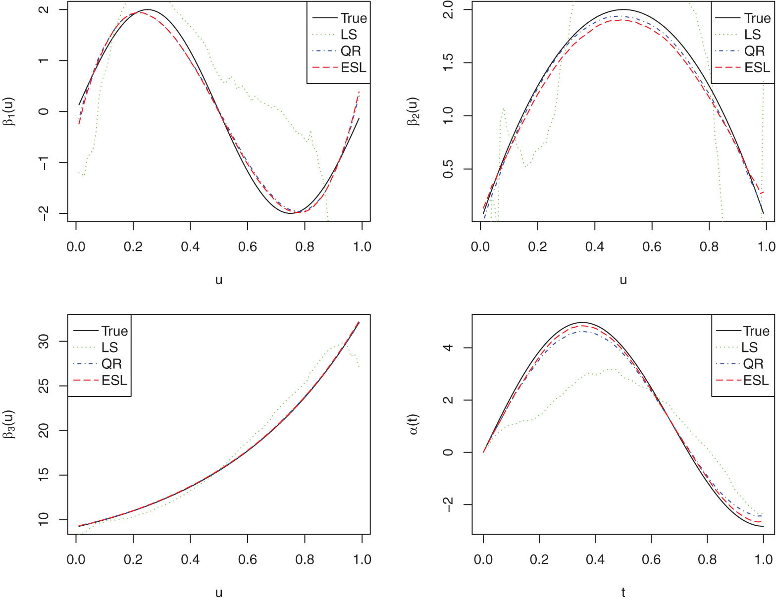
The estimated curves of functions
To further compare the efficiency of the LS, QR, and ESL estimation of the nonparametric functions
where
Mean values of the RT values
|
|
Method |
|
|
|
|---|---|---|---|---|
| 100 | LS | 1 | 1 | 1 |
| QR | 0.8919 | 1.1438 | 2.0084 | |
| ESL | 0.9515 | 1.1743 | 2.4272 | |
| 200 | LS | 1 | 1 | 1 |
| QR | 0.8646 | 1.1153 | 2.0176 | |
| ESL | 0.9245 | 1.1504 | 2.3424 | |
| 600 | LS | 1 | 1 | 1 |
| QR | 0.8821 | 1.1553 | 1.9079 | |
| ESL | 0.9435 | 1.2241 | 2.1859 |
From Table 4, we can see that the RTs of the ESL method are slightly smaller than 1 compared with the RTs of the QR method when the error is normally distributed, for the other two error distributions, the RTs of the ESL method are greater than 1, which indicates that our proposed estimation method can significantly improve the estimation efficiency.
6 A real data analysis
For illustration purposes, we apply the proposed methodology to analyze the spectral data. The data set contains 215 chopped meat samples, each data sample contains fat, protein, moisture contents, and spectral curve. The three contents are measured in percent and determined by analytic chemistry. The spectral curve consists of 100 wavelengths of absorbance spectrum records. Our main interest is to explore the relationship between fat content and other factors. In the subsequent analysis, we treat the fat content as the response variable
For a fair evaluation, the randomly selected 129 samples are used as training data to build the model, and the remaining 86 observations are left as the validation data for prediction purposes. The prediction performance is measured by the mean squared error proposed by [28], which is defined as
7 Concluding remarks
In this article, we provide a robust and efficient estimation approach for VCPFLRMs based on the ESL function. The varying coefficients are approximated by B-splines, and the slope function is estimated by the FPC basis. The theoretical properties of proposed estimators are established under some conditions. Furthermore, we develop a computation algorithm to solve the optimization problems and then introduce a data-driven procedure to select the tuning parameters. The outstanding feature of the newly proposed method is that it can achieve good performance for a wide class of errors by selecting an appropriate tuning parameter
Acknowledgements
The authors are grateful to the editor, the associate editor, and the referees, whose comments and suggestions have greatly helped improve this article.
-
Conflict of interest: The authors state no conflict of interest.
Appendix
In the proofs, we use
Proof of Theorem 1
Suppose
Let
This implies that there is a local minimum in the ball
where
Next, we consider
For
As for
one has
Moreover, by Taylor expansion, we have
where
Let
Then, invoking
Observe that
By Condition (C2) and the orthogonality of
and
Then, combining equations (A.2)–(A.4), we have
References
[1] J. Fan and W. Zhang, Statistical methods with varying coefficient models, Stat. Interface 1 (2008), 179–195, https://dx.doi.org/10.4310/SII.2008.v1.n1.a15. Search in Google Scholar
[2] L. Feng, C. Zou, Z. Wang, X. Wei, and B. Chen, Robust spline-based variable selection in varying coefficient model, Metrika 78 (2015), 85–118, https://doi.org/10.1007/s00184-014-0491-y. Search in Google Scholar
[3] C. Guo, H. Yang, and J. Lv, Robust variable selection in high-dimensional varying coefficient models based on weighted composite quantile regression, Statist. 58 (2017), 1009–1033, https://doi.org/10.1007/s00362-015-0736-5. Search in Google Scholar
[4] T. Hastie and R. Tibshirani, Varying-coefficient models, J. R. Stat. Soc. Ser. B. Methodol. 55 (1993), no. 4, 757–796, https://doi.org/10.1111/j.2517-6161.1993.tb01939.x. Search in Google Scholar
[5] J. Huang, C. Wu, and L. Zhou, Varying-coefficient models and basis function approximations for the analysis of repeated measurements, Biometrika 89 (2002), no. 1, 111–128, https://doi.org/10.1093/biomet/89.1.111. Search in Google Scholar
[6] H. Wang and Y. Xia, Shrinkage estimation of the varying coefficient model, J. Amer. Statist. Assoc. 104 (2009), no. 486, 747–757, https://doi.org/10.1198/jasa.2009.0138. Search in Google Scholar
[7] T. Cai and P. Hall, Prediction in functional linear regression, Ann. Statist. 34 (2006), no. 5, 2159–2179, https://doi.org/10.1214/009053606000000830. Search in Google Scholar
[8] T. Cai and M. Yuan, Minimax and adaptive prediction for functional linear regression, J. Amer. Statist. Assoc. 107 (2012), no. 499, 1201–1216, https://doi.org/10.1080/01621459.2012.716337. Search in Google Scholar
[9] H. Cardot, F. Ferraty, and P. Sarda, Spline estimators for the functional linear model, Statist. Sinica 13 (2003), no. 3, 571–591, http://www.jstor.org/stable/24307112. Search in Google Scholar
[10] P. Hall and J. Horowitz, Methodology and convergence rates for functional linear regression, Ann. Statist. 35 (2007), no. 1, 70–91, https://doi.org/10.1214/009053606000000957. Search in Google Scholar
[11] K. Kato, Estimation in functional linear quantile regression, Ann. Statist. 40 (2012), no. 6, 3108–3136, https://doi.org/10.1214/12-AOS1066. Search in Google Scholar
[12] J. Lei, Adaptive global testing for functional linear models, J. Amer. Statist. Assoc. 109 (2014), no. 506, 624–634, https://doi.org/10.1080/01621459.2013.856794. Search in Google Scholar
[13] F. Yao, H. Müller, and J. Wang, Functional linear regression analysis for longitudinal data, Ann. Statist. 33 (2005), no. 6, 2873–2903, https://doi.org/10.1214/009053605000000660. Search in Google Scholar
[14] Q. Peng, J. Zhou, and N. Tang, Varying coefficient partially functional linear regression models, Statist. Papers 57 (2016), 827–841, https://doi.org/10.1007/s00362-015-0681-3. Search in Google Scholar
[15] H. Shin, Partial functional linear regression, J. Statist. Plann. Inference 139 (2009), no. 10, 3405–3418, https://doi.org/10.1016/j.jspi.2009.03.001. Search in Google Scholar
[16] J. Zhou and M. Chen, Spline estimators for semi-functional linear model, Statist. Probab. Lett. 82 (2012), no. 3, 505–513, https://doi.org/10.1016/j.spl.2011.11.027. Search in Google Scholar
[17] S. Feng and L. Xue, Partially functional linear varying coefficient model, Statistics 50 (2016), no. 4, 717–732, https://doi.org/10.1080/02331888.2016.1138954. Search in Google Scholar
[18] X. Wang, Y. Jiang, M. Huang, and H. Zhang, Robust variable selection with exponential squared loss, J. Amer. Statist. Assoc. 108 (2013), no. 502, 632–643, https://doi.org/10.1080/01621459.2013.766613. Search in Google Scholar PubMed PubMed Central
[19] Y. Jiang, Q. Ji, and B. Xie, Robust estimation for the varying coefficient partially nonlinear models, J. Comput. Appl. Math. 326 (2017), 31–43, https://doi.org/10.1016/j.cam.2017.04.028. Search in Google Scholar
[20] Y. Song, L. Jian, and L. Lin, Robust exponential squared loss-based variable selection for high-dimensional single-index varying-coefficient model, J. Comput. Appl. Math. 308 (2016), 330–345, https://doi.org/10.1016/j.cam.2016.05.030. Search in Google Scholar
[21] P. Yu, Z. Zhu, and Z. Zhang, Robust exponential squared loss-based estimation in semi-functional linear regression models, Comput. Stat. 34 (2019), 503–525, https://doi.org/10.1007/s00180-018-0810-2. Search in Google Scholar
[22] J. Lv, H. Yang, and C. Guo, Robust smooth-threshold estimating equations for generalized varying-coefficient partially linear models based on exponential score function, J. Comput. Appl. Math. 280 (2015), 125–140, DOI: https://doi.org/10.1016/j.cam.2014.11.003. 10.1016/j.cam.2014.11.003Search in Google Scholar
[23] L. Horváth and P. Kokoszka, Inference for Functional Data with Applications, Springer, New York, 2012. 10.1007/978-1-4614-3655-3Search in Google Scholar
[24] P. Yu, J. Du, and Z. Zhang, Varying-coefficient partially functional linear quantile regression models, J. Korean Stat. Soc. 46 (2017), no. 3, 462–475, https://doi.org/10.1016/j.jkss.2017.02.001. Search in Google Scholar
[25] W. Yao, B. Lindsay, and R. Li, Local modal regression, J. Nonparametr. Stat. 24 (2012), no. 3, 647–663, https://doi.org/10.1080/10485252.2012.678848. Search in Google Scholar PubMed PubMed Central
[26] J. Fan and R. Li, Variable selection via nonconcave penalized likelihood and its oracle properties, J. Amer. Statist. Assoc. 96 (2001), no. 456, 1348–1360, https://doi.org/10.1198/016214501753382273. Search in Google Scholar
[27] H. Wang, R. Li, and C. Tsai, Tuning parameter selectors for the smoothly clipped absolute deviation method, Biometrika 94 (2007), no. 3, 553–568, https://doi.org/10.1093/biomet/asm053. Search in Google Scholar PubMed PubMed Central
[28] L. Huang, H. Wang, H. Cui, and S. Wang, Sieve M-estimator for a semi-functional linear model, Sci. China Math. 58 (2015), no. 11, 2421–2434, https://doi.org/10.1007/s11425-015-5040-2. Search in Google Scholar
[29] L. Schumaker, Spline Functions: Basic Theory, Wiley, New York, 1981. Search in Google Scholar
© 2022 Jun Sun and Wanrong Liu, published by De Gruyter
This work is licensed under the Creative Commons Attribution 4.0 International License.
Articles in the same Issue
- Regular Articles
- A random von Neumann theorem for uniformly distributed sequences of partitions
- Note on structural properties of graphs
- Mean-field formulation for mean-variance asset-liability management with cash flow under an uncertain exit time
- The family of random attractors for nonautonomous stochastic higher-order Kirchhoff equations with variable coefficients
- The intersection graph of graded submodules of a graded module
- Isoperimetric and Brunn-Minkowski inequalities for the (p, q)-mixed geominimal surface areas
- On second-order fuzzy discrete population model
- On certain functional equation in prime rings
- General complex Lp projection bodies and complex Lp mixed projection bodies
- Some results on the total proper k-connection number
- The stability with general decay rate of hybrid stochastic fractional differential equations driven by Lévy noise with impulsive effects
- Well posedness of magnetohydrodynamic equations in 3D mixed-norm Lebesgue space
- Strong convergence of a self-adaptive inertial Tseng's extragradient method for pseudomonotone variational inequalities and fixed point problems
- Generic uniqueness of saddle point for two-person zero-sum differential games
- Relational representations of algebraic lattices and their applications
- Explicit construction of mock modular forms from weakly holomorphic Hecke eigenforms
- The equivalent condition of G-asymptotic tracking property and G-Lipschitz tracking property
- Arithmetic convolution sums derived from eta quotients related to divisors of 6
- Dynamical behaviors of a k-order fuzzy difference equation
- The transfer ideal under the action of orthogonal group in modular case
- The multinomial convolution sum of a generalized divisor function
- Extensions of Gronwall-Bellman type integral inequalities with two independent variables
- Unicity of meromorphic functions concerning differences and small functions
- Solutions to problems about potentially Ks,t-bigraphic pair
- Monotonicity of solutions for fractional p-equations with a gradient term
- Data smoothing with applications to edge detection
- An ℋ-tensor-based criteria for testing the positive definiteness of multivariate homogeneous forms
- Characterizations of *-antiderivable mappings on operator algebras
- Initial-boundary value problem of fifth-order Korteweg-de Vries equation posed on half line with nonlinear boundary values
- On a more accurate half-discrete Hilbert-type inequality involving hyperbolic functions
- On split twisted inner derivation triple systems with no restrictions on their 0-root spaces
- Geometry of conformal η-Ricci solitons and conformal η-Ricci almost solitons on paracontact geometry
- Bifurcation and chaos in a discrete predator-prey system of Leslie type with Michaelis-Menten prey harvesting
- A posteriori error estimates of characteristic mixed finite elements for convection-diffusion control problems
- Dynamical analysis of a Lotka Volterra commensalism model with additive Allee effect
- An efficient finite element method based on dimension reduction scheme for a fourth-order Steklov eigenvalue problem
- Connectivity with respect to α-discrete closure operators
- Khasminskii-type theorem for a class of stochastic functional differential equations
- On some new Hermite-Hadamard and Ostrowski type inequalities for s-convex functions in (p, q)-calculus with applications
- New properties for the Ramanujan R-function
- Shooting method in the application of boundary value problems for differential equations with sign-changing weight function
- Ground state solution for some new Kirchhoff-type equations with Hartree-type nonlinearities and critical or supercritical growth
- Existence and uniqueness of solutions for the stochastic Volterra-Levin equation with variable delays
- Ambrosetti-Prodi-type results for a class of difference equations with nonlinearities indefinite in sign
- Research of cooperation strategy of government-enterprise digital transformation based on differential game
- Malmquist-type theorems on some complex differential-difference equations
- Disjoint diskcyclicity of weighted shifts
- Construction of special soliton solutions to the stochastic Riccati equation
- Remarks on the generalized interpolative contractions and some fixed-point theorems with application
- Analysis of a deteriorating system with delayed repair and unreliable repair equipment
- On the critical fractional Schrödinger-Kirchhoff-Poisson equations with electromagnetic fields
- The exact solutions of generalized Davey-Stewartson equations with arbitrary power nonlinearities using the dynamical system and the first integral methods
- Regularity of models associated with Markov jump processes
- Multiplicity solutions for a class of p-Laplacian fractional differential equations via variational methods
- Minimal period problem for second-order Hamiltonian systems with asymptotically linear nonlinearities
- Convergence rate of the modified Levenberg-Marquardt method under Hölderian local error bound
- Non-binary quantum codes from constacyclic codes over 𝔽q[u1, u2,…,uk]/⟨ui3 = ui, uiuj = ujui⟩
- On the general position number of two classes of graphs
- A posteriori regularization method for the two-dimensional inverse heat conduction problem
- Orbital stability and Zhukovskiǐ quasi-stability in impulsive dynamical systems
- Approximations related to the complete p-elliptic integrals
- A note on commutators of strongly singular Calderón-Zygmund operators
- Generalized Munn rings
- Double domination in maximal outerplanar graphs
- Existence and uniqueness of solutions to the norm minimum problem on digraphs
- On the p-integrable trajectories of the nonlinear control system described by the Urysohn-type integral equation
- Robust estimation for varying coefficient partially functional linear regression models based on exponential squared loss function
- Hessian equations of Krylov type on compact Hermitian manifolds
- Class fields generated by coordinates of elliptic curves
- The lattice of (2, 1)-congruences on a left restriction semigroup
- A numerical solution of problem for essentially loaded differential equations with an integro-multipoint condition
- On stochastic accelerated gradient with convergence rate
- Displacement structure of the DMP inverse
- Dependence of eigenvalues of Sturm-Liouville problems on time scales with eigenparameter-dependent boundary conditions
- Existence of positive solutions of discrete third-order three-point BVP with sign-changing Green's function
- Some new fixed point theorems for nonexpansive-type mappings in geodesic spaces
- Generalized 4-connectivity of hierarchical star networks
- Spectra and reticulation of semihoops
- Stein-Weiss inequality for local mixed radial-angular Morrey spaces
- Eigenvalues of transition weight matrix for a family of weighted networks
- A modified Tikhonov regularization for unknown source in space fractional diffusion equation
- Modular forms of half-integral weight on Γ0(4) with few nonvanishing coefficients modulo ℓ
- Some estimates for commutators of bilinear pseudo-differential operators
- Extension of isometries in real Hilbert spaces
- Existence of positive periodic solutions for first-order nonlinear differential equations with multiple time-varying delays
- B-Fredholm elements in primitive C*-algebras
- Unique solvability for an inverse problem of a nonlinear parabolic PDE with nonlocal integral overdetermination condition
- An algebraic semigroup method for discovering maximal frequent itemsets
- Class-preserving Coleman automorphisms of some classes of finite groups
- Exponential stability of traveling waves for a nonlocal dispersal SIR model with delay
- Existence and multiplicity of solutions for second-order Dirichlet problems with nonlinear impulses
- The transitivity of primary conjugacy in regular ω-semigroups
- Stability estimation of some Markov controlled processes
- On nonnil-coherent modules and nonnil-Noetherian modules
- N-Tuples of weighted noncommutative Orlicz space and some geometrical properties
- The dimension-free estimate for the truncated maximal operator
- A human error risk priority number calculation methodology using fuzzy and TOPSIS grey
- Compact mappings and s-mappings at subsets
- The structural properties of the Gompertz-two-parameter-Lindley distribution and associated inference
- A monotone iteration for a nonlinear Euler-Bernoulli beam equation with indefinite weight and Neumann boundary conditions
- Delta waves of the isentropic relativistic Euler system coupled with an advection equation for Chaplygin gas
- Multiplicity and minimality of periodic solutions to fourth-order super-quadratic difference systems
- On the reciprocal sum of the fourth power of Fibonacci numbers
- Averaging principle for two-time-scale stochastic differential equations with correlated noise
- Phragmén-Lindelöf alternative results and structural stability for Brinkman fluid in porous media in a semi-infinite cylinder
- Study on r-truncated degenerate Stirling numbers of the second kind
- On 7-valent symmetric graphs of order 2pq and 11-valent symmetric graphs of order 4pq
- Some new characterizations of finite p-nilpotent groups
- A Billingsley type theorem for Bowen topological entropy of nonautonomous dynamical systems
- F4 and PSp (8, ℂ)-Higgs pairs understood as fixed points of the moduli space of E6-Higgs bundles over a compact Riemann surface
- On modules related to McCoy modules
- On generalized extragradient implicit method for systems of variational inequalities with constraints of variational inclusion and fixed point problems
- Solvability for a nonlocal dispersal model governed by time and space integrals
- Finite groups whose maximal subgroups of even order are MSN-groups
- Symmetric results of a Hénon-type elliptic system with coupled linear part
- On the connection between Sp-almost periodic functions defined on time scales and ℝ
- On a class of Harada rings
- On regular subgroup functors of finite groups
- Fast iterative solutions of Riccati and Lyapunov equations
- Weak measure expansivity of C2 dynamics
- Admissible congruences on type B semigroups
- Generalized fractional Hermite-Hadamard type inclusions for co-ordinated convex interval-valued functions
- Inverse eigenvalue problems for rank one perturbations of the Sturm-Liouville operator
- Data transmission mechanism of vehicle networking based on fuzzy comprehensive evaluation
- Dual uniformities in function spaces over uniform continuity
- Review Article
- On Hahn-Banach theorem and some of its applications
- Rapid Communication
- Discussion of foundation of mathematics and quantum theory
- Special Issue on Boundary Value Problems and their Applications on Biosciences and Engineering (Part II)
- A study of minimax shrinkage estimators dominating the James-Stein estimator under the balanced loss function
- Representations by degenerate Daehee polynomials
- Multilevel MC method for weak approximation of stochastic differential equation with the exact coupling scheme
- Multiple periodic solutions for discrete boundary value problem involving the mean curvature operator
- Special Issue on Evolution Equations, Theory and Applications (Part II)
- Coupled measure of noncompactness and functional integral equations
- Existence results for neutral evolution equations with nonlocal conditions and delay via fractional operator
- Global weak solution of 3D-NSE with exponential damping
- Special Issue on Fractional Problems with Variable-Order or Variable Exponents (Part I)
- Ground state solutions of nonlinear Schrödinger equations involving the fractional p-Laplacian and potential wells
- A class of p1(x, ⋅) & p2(x, ⋅)-fractional Kirchhoff-type problem with variable s(x, ⋅)-order and without the Ambrosetti-Rabinowitz condition in ℝN
- Jensen-type inequalities for m-convex functions
- Special Issue on Problems, Methods and Applications of Nonlinear Analysis (Part III)
- The influence of the noise on the exact solutions of a Kuramoto-Sivashinsky equation
- Basic inequalities for statistical submanifolds in Golden-like statistical manifolds
- Global existence and blow up of the solution for nonlinear Klein-Gordon equation with variable coefficient nonlinear source term
- Hopf bifurcation and Turing instability in a diffusive predator-prey model with hunting cooperation
- Efficient fixed-point iteration for generalized nonexpansive mappings and its stability in Banach spaces