A posteriori error estimates of characteristic mixed finite elements for convection-diffusion control problems
-


Abstract
In this article, we consider fully discrete characteristic mixed finite elements for convection-diffusion optimal control problems. We use the characteristic line method to treat the hyperbolic part of the state equation as a directional derivative. The state and the co-state are discretized by the lowest order Raviart-Thomas mixed finite element spaces and the control is approximated by piecewise constant functions. Using some proper duality problems, we derive a posteriori error estimates for the scalar functions. Such estimates are not available in the literature. A numerical example is presented to validate the theoretical results.
1 Introduction
In the recent 30 years, optimal control problems (OCPs) have been extensively utilized in many aspects of modern life such as social, economic, scientific, and engineering numerical simulation [1]. Thus, they must be solved successfully with efficient numerical methods. Among these numerical methods, the finite element method (FEM) is a good choice for solving OCPs governed by partial differential equations (PDEs). There have been extensive studies on convergence or superconvergence of FEMs for OCPs, see [2,3,4, 5,6,7, 8,9]. A systematic introduction of FEM for PDE OCPs can be found in [10,11, 12,13].
Adaptive FEM has been investigated extensively. It has become one of the most popular methods in cientific computation and numerical modeling. It ensures a higher density of nodes in a certain area of the given domain, where the solution is more difficult to approximate, indicated by a posteriori error estimators. Hence, it is an important approach to boost the accuracy and efficiency of finite element discretization. There is a lot of work concentrating on the adaptivity of various OCPs. For example, [14,15, 16,17,18, 19,20].
In flow control problem or temperature control problem, their objective functional contains not only the state variable but also its gradient. At this moment, the accuracy of the gradient is important in the numerical discretization of the coupled state equations. The mixed finite element method (MFEM) is appropriate for the state equations in such cases since both the scalar variable and its flux variable can be approximated to the same accuracy, for example, [21,22,23, 24,25].
Recently, more and more attention has been paid to elliptic convection-diffusion OCPs [26,27,28]. Fu and Rui have studied a priori and a posteriori error estimates of characteristic finite element methods (CFEMs) for time-dependent convection-diffusion OCPs in [29] and [30], respectively. They also considered a priori error estimates of characteristic mixed finite element method (CMFEM) for time-dependent convection-diffusion OCPs in [31]. In [32], Sun and Ma investigated a nonoverlapping domain decomposition method combined with the characteristic method for OCPs governed by parabolic convection-diffusion equations.
In this work, we consider a posteriori error estimates of fully discrete CMFEM for OCPs governed by convection-diffusion equations. The characteristic approximation is applied to handle the convection term, and the lowest order RT mixed finite element spatial approximation is adopted to deal with the diffusion term. The OCPs that we are interested in are as follows:
where
Moreover, we assume that the constraint on the control is an obstacle such that
In this article, we adopt the standard notation
We denote by
The plan of this article is as follows. In Section 2, we shall construct a CMFEM approximation for the OCPs (1)–(5). In Section 3, we derive a posteriori
2 CMFEM approximation of convection-diffusion OCPs
In this section, we shall construct a CMFEM and backward Euler discretization approximation of convection-diffusion OCPs (1)–(5). To fix the idea, we shall take the state spaces
The Hilbert space
Now, we take account of the hyperbolic part of (2), namely
Then equation (2) is equivalent to the following form:
We recast (1)–(5) as the following weak form: find
It follows from [1] that the OCPs (6)–(9) have a unique solution
where
We now consider the time discretization. Let
Let
We denote by
Next, we use the MFEM for spatial discretization. Let
Then a fully discrete CMFEM approximation of (6)–(9) is to find
where
It follows from [31] that the control problem (17)–(20) has a unique solution
where
We denote by
since the flow is incompressible, i.e.,
For
For
For any function
Moreover, we let
Then the optimality conditions (21)–(27) satisfying
In the rest of the article, we shall use some intermediate variables. For any control function
Let
Let
where
We have the commuting diagram property
where and after,
Furthermore, the interpolation operator
3 A posteriori error estimates
In this section, we derive a posteriori error estimates of fully discrete CMFEM for parabolic convection-diffusion OCPs. In order to the following analysis, we divide the domain
It is easy to see that the partition of the above three subsets is dependent on
First, let us derive the a posteriori error estimates for the control
Theorem 3.1
Let
where
Proof
It follows from (19) that
We first estimate
It follows from Hölder’s inequality and Young’s inequality that
Furthermore, we have that
It yields that
Moreover, it is clear that
Now we turn to
Then from (10)–(15) and (37)–(42), we have
In order to estimate the error
and
Lemma 3.1
[36] Let
where
Lemma 3.2
[37] Let f and g be piecewise continuous nonnegative functions defined on
then
In the following two theorems, we shall estimate the error
Theorem 3.2
Let
where
Proof
From (31), we can obtain the following equality:
Let
Using (30), (43), Cauchy inequality, and Lemma 3.1, we have
Similarly, using Cauchy inequality, and Lemma 3.1, we derive
Finally, for
Theorem 3.3
Let
where
Proof
Similar to (61), using (34) and the definitions of
Let
First, using the same estimates as (63)–(66), we have
For
Finally, for
Therefore, the above estimates and the triangle inequality yield (68).□
Let
From (10)–(16) and (37)–(42), we derive the following error equations:
Theorem 3.4
There is a constant
Proof
Choosing
Then, using
Note that
then, using the assumption on
Integrating (86) in time and since
this implies (82).
Similarly, we can obtain
Using (88) and (82), we complete the proof of Theorem 3.4.□
Collecting Theorems 3.1–3.4, we can derive the following results:
Theorem 3.5
Let
where
4 Numerical experiments
In this section, we illustrate our theoretical results by a numerical example.
For a constrained optimization problem:
where
where
By applying (90) to the fully discretized problem (21)–(27), for an acceptable error
Algorithm 4.1. Projection gradient algorithm
Step 1. Initialize
Step 2. Solve the following equations:
Step 3. Calculate the iterative error:
Step 4. If
Algorithm 4.2. Adaptive projection gradient algorithm
Step 1. Solve the discretized optimization problem (21)–(27) with Algorithm 4.1 on the current mesh (the same mesh is used for the control, state, and co-state variables), obtain numerical solution
Step 2. Adjust the mesh by
Step 3. Calculate the iterative error:
Step 4. If
The following numerical example was solved with the C++ software package: AFEPack which is freely available. Let
Example 1. The data are as follows:
It is clear that the optimal control has a strong discontinuity along the diagonal
Some numerical results are shown in Table 1, where the numerical results based on uniform refined mesh and adaptively refined mesh are obtained by Algorithms 4.1 and 4.2, respectively. The errors
Numerical results based on uniform and adaptive meshes
| Mesh info | Uniform mesh | Adaptive mesh | ||||
|---|---|---|---|---|---|---|
|
|
|
|
|
|
|
|
| Nodes | 7,617 | 7,617 | 7,617 | 1,737 | 1,737 | 1,737 |
| Sides | 22,528 | 22,528 | 22,528 | 4,597 | 4,597 | 4,597 |
| Elements | 14,912 | 14,912 | 14,912 | 2,861 | 2,861 | 2,861 |
| Dofs | 14,912 | 14,912 | 14,912 | 2,861 | 2,861 | 2,861 |
|
|
|
|
|
|
|
|
We plot the profile of the exact solution
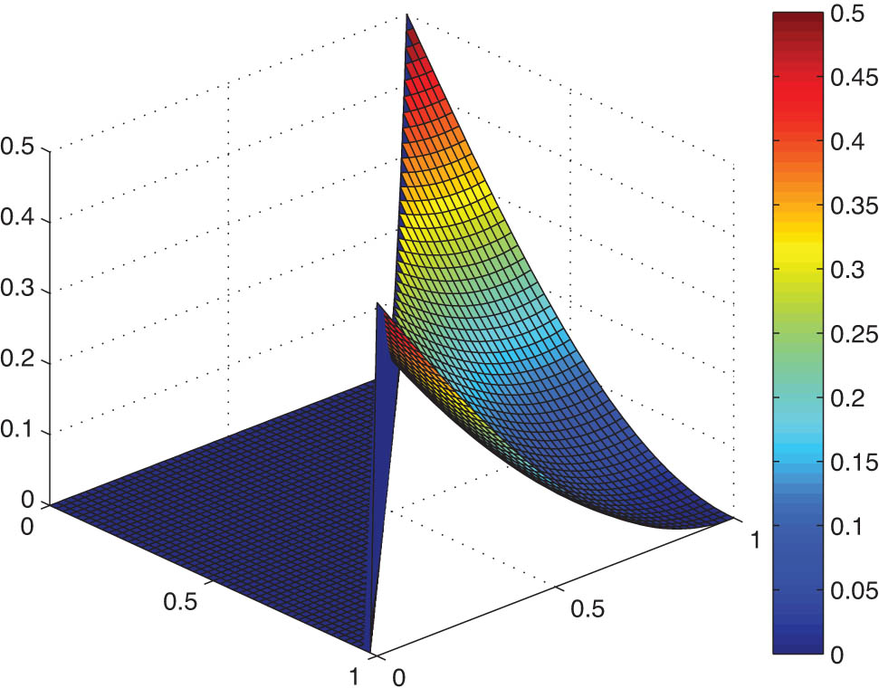
The exact solution
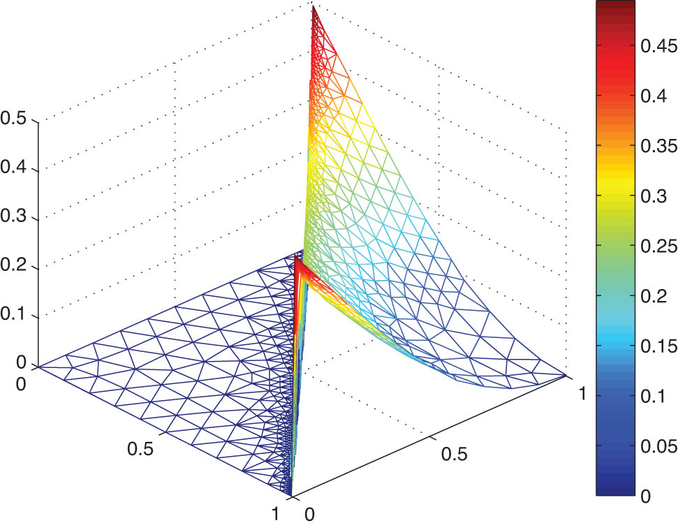
The numerical solution
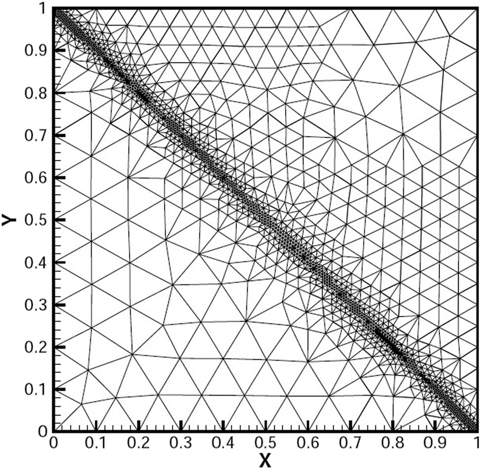
The adaptive mesh for
5 Conclusion
In this article, we consider a fully discrete CMFEM for parabolic convection-diffusion OCPs. We derive a posteriori
-
Funding information: Yuelong Tang is supported by the National Natural Science Foundation of China (11401201), the Natural Science Foundation of Hunan Province (2020JJ4323), the Scientific Research Project of Hunan Provincial Department of Education (20A211), and the construct program of applied characteristic discipline in Hunan University of Science and Engineering. Yuchun Hua is supported by the Scientific Research Project of Hunan Provincial Department of Education (20C0854) and the scientific research program in Hunan University of Science and Engineering (20XKY059).
-
Conflict of interest: The authors state no conflict of interest.
References
[1] J. Lions, Optimal Control of Systems Governed by Partial Differential Equations, Springer, Berlin, 1971. 10.1007/978-3-642-65024-6Search in Google Scholar
[2] L. Hou and J. Turner, Analysis and finite element approximation of an optimal control problem in electrochemistry with current density controls, Numer. Math. 71 (1995), 289–315. 10.1007/s002110050146Search in Google Scholar
[3] G. Knowles, Finite element approximation of parabolic time optimal control problems, SIAM J. Control Optim. 20 (1982), 414–427. 10.1137/0320032Search in Google Scholar
[4] R. Mcknight and W. Bosarge, The Ritz-Galerkin procedure for parabolic control problems, SIAM J. Control Optim. 11 (1973), 510–524. 10.1137/0311040Search in Google Scholar
[5] N. Arada, E. Casas, and F. Tröltzsch, Error estimates for the numerical approximation of a semilinear elliptic control problem, Comput. Optim. Appl. 23 (2002), 201–229. 10.1023/A:1020576801966Search in Google Scholar
[6] Y. Tang and Y. Chen, Superconvergence analysis of fully discrete finite element methods for semilinear parabolic optimal control problems, Front. Math. China 8 (2013), no. 2, 443–464. 10.1007/s11464-013-0239-4Search in Google Scholar
[7] Y. Tang and Y. Hua, Superconvergence analysis for parabolic optimal control problems, Calcolo 51 (2014), 381–392. 10.1007/s10092-013-0091-7Search in Google Scholar
[8] Y. Tang and Y. Hua, Superconvergence of splitting positive definite mixed finite element for parabolic optimal control problems, Appl. Anal. 97 (2018), no. 16, 2778–2793. 10.1080/00036811.2017.1392014Search in Google Scholar
[9] Y. Hua and Y. Tang, A splitting positive definite mixed finite element method for parabolic control problems with integral constraints, J. Nonlinear Funct. Anal. 35 (2021), 1–15. Search in Google Scholar
[10] W. Liu and N. Yan, Adaptative Finite Element Methods for Optimal Control Governed by PDEs, Scientific Press, Beijing, 2008. Search in Google Scholar
[11] Y. Chen and Z. Lu, High Efficient and Accuracy Numerical Methods for Optimal Control Problems, Science Press, Beijing, 2015. Search in Google Scholar
[12] P. Neittaanmaki and D. Tiba, Optimal Control of Nonlinear Parabolic Systems: Theory, Algorithms and Applications, Marcel Dekker INC., New York, 1994. Search in Google Scholar
[13] D. Tiba, Lectures on the Optimal Control of Elliptic Problems, University of Jyvaskyla Press, Jyvaskyla, 1995. Search in Google Scholar
[14] W. Liu, H. Ma, T. Tang, and N. Yan, A posteriori error estimates for discontinuous Galerkin time-stepping method for optimal control problems governed by parabolic equations, SIAM J. Numer. Anal. 42 (2004), 1032–1061. 10.1137/S0036142902397090Search in Google Scholar
[15] R. Becker, H. Kapp, and R. Rannacher, Adaptive finite element methods for optimal control of partial differential equations: Basic concept, SIAM J. Control Optim. 39 (2000), 113–132. 10.1137/S0363012999351097Search in Google Scholar
[16] H. Brunner and N. Yan, Finite element methods for optimal control problems governed by integral equations and integro-differential equations, Numer. Math. 101 (2005), 1–27. 10.1007/s00211-005-0608-3Search in Google Scholar
[17] W. Gong and N. Yan, A posteriori error estimate for boundary control problems governed by the parabolic partial differential equations, J. Comput. Math. 27 (2009), 68–88. Search in Google Scholar
[18] R. Hoppe, Y. Iliash, C. Iyyunni, and N. Sweilam, A posteriori error estimates for adaptive finite element discretizations of boundary control problems, J. Numer. Math. 14 (2006), 57–82. 10.1163/156939506776382139Search in Google Scholar
[19] W. Liu and N. Yan, A posteriori error estimates for optimal control problems governed by parabolic equations, Numer. Math. 93 (2003), 497–521. 10.1007/s002110100380Search in Google Scholar
[20] R. Li, W. Liu, H. Ma, and T. Tang, Adaptive finite element approximation of elliptic control problems, SIAM J. Control Optim. 41 (2002), 1321–1349. 10.1137/S0363012901389342Search in Google Scholar
[21] Y. Chen, Superconvergence of quadratic optimal control problems by triangular mixed finite elements, Inter. J. Numer. Meth. Eng. 75 (2008), 881–898. 10.1002/nme.2272Search in Google Scholar
[22] Y. Chen, Y. Huang, W. Liu, and N. Yan, Error estimates and superconvergence of mixed finite element methods for convex optimal control problems, J. Sci. Comput. 42 (2009), 382–403. 10.1007/s10915-009-9327-8Search in Google Scholar
[23] Y. Chen and W. Liu, A posteriori error estimates for mixed finite element solutions of convex optimal control problems, J. Comput. Appl. Math. 211 (2008), 76–89. 10.1016/j.cam.2006.11.015Search in Google Scholar
[24] Z. Lu and S. Zhang, Linfty-error estimates of rectangular mixed finite element methods for bilinear optimal control problem, Appl. Math. Comput. 300 (2017), 79–94. 10.1016/j.amc.2016.12.006Search in Google Scholar
[25] Y. Chen, Z. Lu, and Y. Huang, Superconvergence of triangular Raviart-Thomas mixed finite element methods for bilinear constrained optimal control problem, Comput. Math. Appl. 66 (2013), 1498–1513. 10.1016/j.camwa.2013.08.019Search in Google Scholar
[26] D. Gathungu and A. Borzi, A multigrid scheme for solving convection-diffusion-integral optimal control problems, Comput. Visual Sci. 22 (2019), 43–55. 10.1007/s00791-017-0285-7Search in Google Scholar
[27] M. Darehmiraki, A. Rezazadeh, A. Ahmadian, and S. Salahshour, An interpolation method for the optimal control problem governed by the elliptic convection-diffusion equation, Numer. Methods Partial Differential Equations 2020 (2020), 1–23, https://doi.org/10.1002/num.22625. Search in Google Scholar
[28] F. Samadi, A. Heydari, and S. Effati, A numerical method based on a bilinear pseudo-spectral method to solve the convection-diffusion optimal control problems, Inter. J. Comput. Math. 98 (2021), no. 1, 28–46. 10.1080/00207160.2020.1723563Search in Google Scholar
[29] H. Fu, A characteristic finite element method for optimal control problems governed by convection-diffusion equations, J. Comput. Appl. Math. 235 (2010), 825–836. 10.1016/j.cam.2010.07.010Search in Google Scholar
[30] H. Fu and H. Rui, Adaptive characteristic finite element approximation of convection-diffusion optimal control problems, Numer. Methods Partial Differential Equations 29 (2013), 979–998. 10.1002/num.21741Search in Google Scholar
[31] H. Fu and H. Rui, A characteristic-mixed finite element method for time-dependent convection-diffusion optimal control problem, Appl. Math. Comput. 218 (2011), 3430–3440. 10.1016/j.amc.2011.08.087Search in Google Scholar
[32] T. Sun and K. Ma, A non-overlapping DDM combined with the characteristic method for optimal control problems governed by convection-diffusion equations, Comput. Optim. Appl. 71 (2018), 273–306. 10.1007/s10589-018-0008-0Search in Google Scholar
[33] F. Brezzi and M. Fortin, Mixed and Hybrid Finite Element Methods, Springer-Verlag, Berlin, 1999. Search in Google Scholar
[34] I. Babuska and T. Strouboulis, The Finite Element Method and Its Reliability, Oxford University Press, Oxford, 2001. 10.1093/oso/9780198502760.001.0001Search in Google Scholar
[35] C. Carstensen, A posteriori error estimate for the mixed finite element method, Math. Comp. 66 (1997), 465–476. 10.1090/S0025-5718-97-00837-5Search in Google Scholar
[36] P. Houston and E. Suli, Adaptive Lagrange-Galerkin methods for unsteady convection-diffusion problems, Math. Comp. 70 (2000), 77–106. 10.1090/S0025-5718-00-01187-XSearch in Google Scholar
[37] V. Thomée, Galerkin Finite Element Methods for Parabolic Problems, Springer-Verlag, Berlin, 1997. 10.1007/978-3-662-03359-3Search in Google Scholar
[38] R. Li, W. Liu, and N. Yan, A posteriori error estimates of recovery type for distributed convex optimal control problems, J. Sci. Comput. 33 (2007), 155–182. 10.1007/s10915-007-9147-7Search in Google Scholar
© 2022 Yuelong Tang and Yuchun Hua, published by De Gruyter
This work is licensed under the Creative Commons Attribution 4.0 International License.
Articles in the same Issue
- Regular Articles
- A random von Neumann theorem for uniformly distributed sequences of partitions
- Note on structural properties of graphs
- Mean-field formulation for mean-variance asset-liability management with cash flow under an uncertain exit time
- The family of random attractors for nonautonomous stochastic higher-order Kirchhoff equations with variable coefficients
- The intersection graph of graded submodules of a graded module
- Isoperimetric and Brunn-Minkowski inequalities for the (p, q)-mixed geominimal surface areas
- On second-order fuzzy discrete population model
- On certain functional equation in prime rings
- General complex Lp projection bodies and complex Lp mixed projection bodies
- Some results on the total proper k-connection number
- The stability with general decay rate of hybrid stochastic fractional differential equations driven by Lévy noise with impulsive effects
- Well posedness of magnetohydrodynamic equations in 3D mixed-norm Lebesgue space
- Strong convergence of a self-adaptive inertial Tseng's extragradient method for pseudomonotone variational inequalities and fixed point problems
- Generic uniqueness of saddle point for two-person zero-sum differential games
- Relational representations of algebraic lattices and their applications
- Explicit construction of mock modular forms from weakly holomorphic Hecke eigenforms
- The equivalent condition of G-asymptotic tracking property and G-Lipschitz tracking property
- Arithmetic convolution sums derived from eta quotients related to divisors of 6
- Dynamical behaviors of a k-order fuzzy difference equation
- The transfer ideal under the action of orthogonal group in modular case
- The multinomial convolution sum of a generalized divisor function
- Extensions of Gronwall-Bellman type integral inequalities with two independent variables
- Unicity of meromorphic functions concerning differences and small functions
- Solutions to problems about potentially Ks,t-bigraphic pair
- Monotonicity of solutions for fractional p-equations with a gradient term
- Data smoothing with applications to edge detection
- An ℋ-tensor-based criteria for testing the positive definiteness of multivariate homogeneous forms
- Characterizations of *-antiderivable mappings on operator algebras
- Initial-boundary value problem of fifth-order Korteweg-de Vries equation posed on half line with nonlinear boundary values
- On a more accurate half-discrete Hilbert-type inequality involving hyperbolic functions
- On split twisted inner derivation triple systems with no restrictions on their 0-root spaces
- Geometry of conformal η-Ricci solitons and conformal η-Ricci almost solitons on paracontact geometry
- Bifurcation and chaos in a discrete predator-prey system of Leslie type with Michaelis-Menten prey harvesting
- A posteriori error estimates of characteristic mixed finite elements for convection-diffusion control problems
- Dynamical analysis of a Lotka Volterra commensalism model with additive Allee effect
- An efficient finite element method based on dimension reduction scheme for a fourth-order Steklov eigenvalue problem
- Connectivity with respect to α-discrete closure operators
- Khasminskii-type theorem for a class of stochastic functional differential equations
- On some new Hermite-Hadamard and Ostrowski type inequalities for s-convex functions in (p, q)-calculus with applications
- New properties for the Ramanujan R-function
- Shooting method in the application of boundary value problems for differential equations with sign-changing weight function
- Ground state solution for some new Kirchhoff-type equations with Hartree-type nonlinearities and critical or supercritical growth
- Existence and uniqueness of solutions for the stochastic Volterra-Levin equation with variable delays
- Ambrosetti-Prodi-type results for a class of difference equations with nonlinearities indefinite in sign
- Research of cooperation strategy of government-enterprise digital transformation based on differential game
- Malmquist-type theorems on some complex differential-difference equations
- Disjoint diskcyclicity of weighted shifts
- Construction of special soliton solutions to the stochastic Riccati equation
- Remarks on the generalized interpolative contractions and some fixed-point theorems with application
- Analysis of a deteriorating system with delayed repair and unreliable repair equipment
- On the critical fractional Schrödinger-Kirchhoff-Poisson equations with electromagnetic fields
- The exact solutions of generalized Davey-Stewartson equations with arbitrary power nonlinearities using the dynamical system and the first integral methods
- Regularity of models associated with Markov jump processes
- Multiplicity solutions for a class of p-Laplacian fractional differential equations via variational methods
- Minimal period problem for second-order Hamiltonian systems with asymptotically linear nonlinearities
- Convergence rate of the modified Levenberg-Marquardt method under Hölderian local error bound
- Non-binary quantum codes from constacyclic codes over 𝔽q[u1, u2,…,uk]/⟨ui3 = ui, uiuj = ujui⟩
- On the general position number of two classes of graphs
- A posteriori regularization method for the two-dimensional inverse heat conduction problem
- Orbital stability and Zhukovskiǐ quasi-stability in impulsive dynamical systems
- Approximations related to the complete p-elliptic integrals
- A note on commutators of strongly singular Calderón-Zygmund operators
- Generalized Munn rings
- Double domination in maximal outerplanar graphs
- Existence and uniqueness of solutions to the norm minimum problem on digraphs
- On the p-integrable trajectories of the nonlinear control system described by the Urysohn-type integral equation
- Robust estimation for varying coefficient partially functional linear regression models based on exponential squared loss function
- Hessian equations of Krylov type on compact Hermitian manifolds
- Class fields generated by coordinates of elliptic curves
- The lattice of (2, 1)-congruences on a left restriction semigroup
- A numerical solution of problem for essentially loaded differential equations with an integro-multipoint condition
- On stochastic accelerated gradient with convergence rate
- Displacement structure of the DMP inverse
- Dependence of eigenvalues of Sturm-Liouville problems on time scales with eigenparameter-dependent boundary conditions
- Existence of positive solutions of discrete third-order three-point BVP with sign-changing Green's function
- Some new fixed point theorems for nonexpansive-type mappings in geodesic spaces
- Generalized 4-connectivity of hierarchical star networks
- Spectra and reticulation of semihoops
- Stein-Weiss inequality for local mixed radial-angular Morrey spaces
- Eigenvalues of transition weight matrix for a family of weighted networks
- A modified Tikhonov regularization for unknown source in space fractional diffusion equation
- Modular forms of half-integral weight on Γ0(4) with few nonvanishing coefficients modulo ℓ
- Some estimates for commutators of bilinear pseudo-differential operators
- Extension of isometries in real Hilbert spaces
- Existence of positive periodic solutions for first-order nonlinear differential equations with multiple time-varying delays
- B-Fredholm elements in primitive C*-algebras
- Unique solvability for an inverse problem of a nonlinear parabolic PDE with nonlocal integral overdetermination condition
- An algebraic semigroup method for discovering maximal frequent itemsets
- Class-preserving Coleman automorphisms of some classes of finite groups
- Exponential stability of traveling waves for a nonlocal dispersal SIR model with delay
- Existence and multiplicity of solutions for second-order Dirichlet problems with nonlinear impulses
- The transitivity of primary conjugacy in regular ω-semigroups
- Stability estimation of some Markov controlled processes
- On nonnil-coherent modules and nonnil-Noetherian modules
- N-Tuples of weighted noncommutative Orlicz space and some geometrical properties
- The dimension-free estimate for the truncated maximal operator
- A human error risk priority number calculation methodology using fuzzy and TOPSIS grey
- Compact mappings and s-mappings at subsets
- The structural properties of the Gompertz-two-parameter-Lindley distribution and associated inference
- A monotone iteration for a nonlinear Euler-Bernoulli beam equation with indefinite weight and Neumann boundary conditions
- Delta waves of the isentropic relativistic Euler system coupled with an advection equation for Chaplygin gas
- Multiplicity and minimality of periodic solutions to fourth-order super-quadratic difference systems
- On the reciprocal sum of the fourth power of Fibonacci numbers
- Averaging principle for two-time-scale stochastic differential equations with correlated noise
- Phragmén-Lindelöf alternative results and structural stability for Brinkman fluid in porous media in a semi-infinite cylinder
- Study on r-truncated degenerate Stirling numbers of the second kind
- On 7-valent symmetric graphs of order 2pq and 11-valent symmetric graphs of order 4pq
- Some new characterizations of finite p-nilpotent groups
- A Billingsley type theorem for Bowen topological entropy of nonautonomous dynamical systems
- F4 and PSp (8, ℂ)-Higgs pairs understood as fixed points of the moduli space of E6-Higgs bundles over a compact Riemann surface
- On modules related to McCoy modules
- On generalized extragradient implicit method for systems of variational inequalities with constraints of variational inclusion and fixed point problems
- Solvability for a nonlocal dispersal model governed by time and space integrals
- Finite groups whose maximal subgroups of even order are MSN-groups
- Symmetric results of a Hénon-type elliptic system with coupled linear part
- On the connection between Sp-almost periodic functions defined on time scales and ℝ
- On a class of Harada rings
- On regular subgroup functors of finite groups
- Fast iterative solutions of Riccati and Lyapunov equations
- Weak measure expansivity of C2 dynamics
- Admissible congruences on type B semigroups
- Generalized fractional Hermite-Hadamard type inclusions for co-ordinated convex interval-valued functions
- Inverse eigenvalue problems for rank one perturbations of the Sturm-Liouville operator
- Data transmission mechanism of vehicle networking based on fuzzy comprehensive evaluation
- Dual uniformities in function spaces over uniform continuity
- Review Article
- On Hahn-Banach theorem and some of its applications
- Rapid Communication
- Discussion of foundation of mathematics and quantum theory
- Special Issue on Boundary Value Problems and their Applications on Biosciences and Engineering (Part II)
- A study of minimax shrinkage estimators dominating the James-Stein estimator under the balanced loss function
- Representations by degenerate Daehee polynomials
- Multilevel MC method for weak approximation of stochastic differential equation with the exact coupling scheme
- Multiple periodic solutions for discrete boundary value problem involving the mean curvature operator
- Special Issue on Evolution Equations, Theory and Applications (Part II)
- Coupled measure of noncompactness and functional integral equations
- Existence results for neutral evolution equations with nonlocal conditions and delay via fractional operator
- Global weak solution of 3D-NSE with exponential damping
- Special Issue on Fractional Problems with Variable-Order or Variable Exponents (Part I)
- Ground state solutions of nonlinear Schrödinger equations involving the fractional p-Laplacian and potential wells
- A class of p1(x, ⋅) & p2(x, ⋅)-fractional Kirchhoff-type problem with variable s(x, ⋅)-order and without the Ambrosetti-Rabinowitz condition in ℝN
- Jensen-type inequalities for m-convex functions
- Special Issue on Problems, Methods and Applications of Nonlinear Analysis (Part III)
- The influence of the noise on the exact solutions of a Kuramoto-Sivashinsky equation
- Basic inequalities for statistical submanifolds in Golden-like statistical manifolds
- Global existence and blow up of the solution for nonlinear Klein-Gordon equation with variable coefficient nonlinear source term
- Hopf bifurcation and Turing instability in a diffusive predator-prey model with hunting cooperation
- Efficient fixed-point iteration for generalized nonexpansive mappings and its stability in Banach spaces