Phragmén-Lindelöf alternative results and structural stability for Brinkman fluid in porous media in a semi-infinite cylinder
-
Yuanfei Li
 and
Xuejiao Chen
and
Xuejiao Chen

Abstract
This article investigates the spatial behavior of the solutions of the Brinkman equations in a semi-infinite cylinder. We no longer require the solutions to satisfy any a priori assumptions at infinity. Using the energy estimation method and the differential inequality technology, the differential inequality about the solutions is derived. By solving this differential inequality, it is proved that the solutions grow polynomially or decay exponentially with spatial variables. In the case of decay, the structural stability of Brinkman fluid is also proved.
1 Introduction
The Brinkman equations are often used to describe flow in a porous medium, which have been discussed in the books of Nield and Bejan [1], Straughan [2], and Hewitt [3]. Many scholars in the literature have paid attention to the spatial attenuation of Brinkman equations on a semi-infinite cylinder. Payne and Song [4] considered the fluid in porous media controlled by Brinkman equations. The Saint-Venant-type decay of the solutions on a semi-infinite cylinder is obtained. For more works on fluid equations, one can see [5,6, 7,8,9, 10,11]. These articles need to assume that the solutions satisfy certain a priori assumptions at the infinity of the cylinder.
However, the classical Phragmén-Lindelöf alternative theorem does not need such a priori assumption, but proves that the solutions either decay exponentially or increase exponentially with the distance from the finite end of the cylinder. In the past few decades, the Phragmén-Lindelöf alternative research has received a lot of attention (see [12,13,14, 15,16,17]). The above articles mainly focus on linear problems.
In this article, we suppose that a porous medium occupies the interior of a semi-infinite cylindrical pipe of arbitrary cross-section and generators parallel to the
where
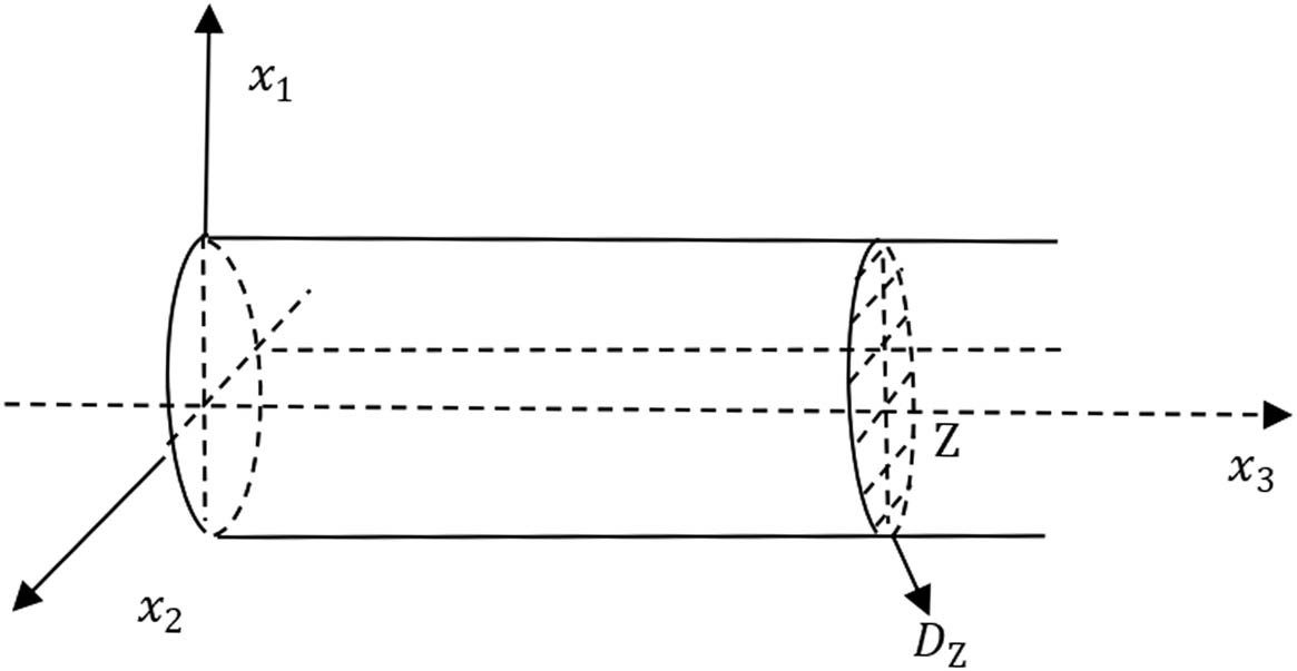
Cylindrical pipe.
The Brinkman equations we consider in this article can be written as follows:
where
We use commas for derivation, repeated English subscripts for summation from 1 to 3, and repeated Greek subscripts for summation from 1 to 2, e.g.,
Equations (1.1)–(1.3) also satisfy the following initial-boundary conditions:
where
We also introduce the following notations:
where
This article studies the Phragmén-Lindelöf-type alternative theorem of equations (1.1)–(1.7) on
2 Preliminary
Here are some lemmas that will be often used.
Lemma 2.1
[4] If
where
where
Lemma 2.2
[30] There exists a positive constant
Lemma 2.3
[31] If g is a continuously differentiable function on D and
and a positive constant C depending only on the geometry of D such that
To obtain the Phragmén-Lindelöf-type alternative result of the solutions to (1.1)–(1.3), we define
where
In (2.2)–(2.4),
Second, differentiating equation (1.1) with respect to
Therefore, we have
By the divergence theorem, we have from (2.6)
We have, from (2.7) and (2.3),
Similar to (2.5), we have
Combining (2.2), (2.3), and (2.4), we have
Combining (2.5), (2.8), and (2.9), we have
From (2.11), we have
We have the following lemma.
Lemma 2.4
For the function
where
Proof
Using the Hölder inequality and the Young inequality, we have
Inserting (2.14) into (2.15) and choosing
and
Next, we will bound
This shows that the area mean value of
Therefore, using (1.1), we have
Using the Hölder inequality, the Young inequality, and Lemmas 2.1 and 2.3, we have
Inserting (2.19)–(2.22) into (2.18) and noting (2.16), we have
where we have used the condition
For
Using the Hölder inequality and the Young inequality, we have
Inserting (2.25)–(2.28) into (2.24), we have
Using the Hölder inequality and the Young inequality, we have
Combining (2.30)–(2.33), we have
Using the Hölder inequality, the Young inequality, and Lemma 2.2, we have
Inserting (2.23), (2.29), (2.34), and (2.35) into (2.10), we can obtain Lemma 2.4.□
3 Main result
Based on Lemma 4, we can obtain the following theorem.
Theorem 3.1
Let
holds or
holds, where
Proof
We consider (2.1) for two cases.
Case I.
From (2.11), we know that
Using the Young inequality, we have
Inserting (3.4) into (3.3), we have
where
From (3.5), it follows that
So, we have
Integrating (3.6) from
We discard the second and third terms at the left end of (3.7). In the first term of (3.7), we use the following inequality:
to have
Therefore, we have
On the other hand, we integrate (2.12) from
Combining (3.8) and (3.9), we can obtain (3.1).
Case II.
Using the Young inequality again, we have
Inserting (3.11) into (3.10), we have
where
So, we have
Integrating (3.13) from 0 to
Dropping the first term on the left of (3.14), we have
Therefore, we obtain
where
Squaring (3.15), we have
So, we have
4 Continuous dependence result
In this section, we derive the continuous dependence on the Brinkman coefficient
Lemma 4.1
(See [32]) Let
and
Suppose that
then
Next, we derive the continuous dependence result.
We multiply (4.2) with
from which it follows that
Using the Schwarz inequality and (3.2), we obtain
Obviously,
Using the Schwarz inequality and Lemma 4.1, we obtain
Inserting (4.12)–(4.15) into (4.11), we have
Using the Schwarz inequality, we obtain
Inserting (4.9), (4.10), and (4.16)–(4.18) into (4.8), we have
Now, we multiply (4.4) with
from which it follows that
Using the Schwarz inequality, we obtain
Using Lemma 2.2, we have
Let
we have
Inserting (4.21)–(4.24) into (4.20), we have
If we define
then we have
Combining (4.19) and (4.25) and choosing
where
In view of (3.2), we have
Therefore,
Inserting (4.30) and (4.31) into (4.28), we have
where
If
If
If
To obtain the main result, we have to derive the upper bound for
Therefore, we only need to derive the bound for
On the other hand, combining (4.8) and (4.20) and using the initial-boundary conditions (4.5)–(4.7), we obtain
Since
Therefore, we have
Inserting (4.40) into (4.37), we have
where
Theorem 4.1
Let
If
If
5 Conclusion
In this article, we define the Brinkman equations (1.1)–(1.3) in a semi-infinite cylinder and the Phragmén-Lindelöf alternative result and the continuous dependence result on
Li et al. [17,33] studied the selectivity of the wave equations in the region
-
Funding information: This work is supported by the Key projects of universities in Guangdong Province (Natural Science) (2019KZDXM042) and the Research team project of Guangzhou Huashang College(2021HSKT01).
-
Author contributions: All authors have accepted responsibility for the entire content of this manuscript and approved its submission.
-
Conflict of interest: The authors state that there is no conflict of interest.
-
Data availability statement: This article focuses on theoretical analysis, not involving experiments and data.
References
[1] D. A. Nield and A. Bejan, Convection in Porous Media, Springer-Verlag, New York, 1992. 10.1007/978-1-4757-2175-1Search in Google Scholar
[2] B. Straughan, Mathematical aspects of penetrative convection, Pitman Res. Notes Math. Vol. 288, Longman, Harlow, 1993. Search in Google Scholar
[3] D. R. Hewitt, Vigorous convection in porous media, Proc. R. Soc. A: Math. Phys. Eng. Sci. 476 (2020), no. 2239, 20200111, https://doi.org/10.1098/rspa.2020.0111. Search in Google Scholar PubMed PubMed Central
[4] L. E. Payne and J. C. Song, Spatial decay estimates for the Brinkman and Darcy flows in a semi-infinite cylinder, Contin. Mech. Thermodyn. 9 (1997), 175–190, https://doi.org/10.1007/s001610050064. Search in Google Scholar
[5] Y. F. Li, Y. Liu, S. Luo, and C. Lin, Decay Estimates for the Brinkman-Forchheimer equations in a semi-infinite pipe, ZAMM Z. Angew. Math. Mech. 92 (2012), no. 2, 160–176, https://doi.org/10.1002/zamm.201000202. Search in Google Scholar
[6] Y. F. Li, Y. Liu, and C. Lin, Decay estimates for homogeneous Boussinesq equations in a semi-infinite pipe, Nonlinear Anal. 74 (2011), no. 13, 4399–4417, https://doi.org/10.1016/j.na.2011.03.062. Search in Google Scholar
[7] Y. F. Li and C. H. Lin, Spatial decay for solutions to 2-D Boussinesq system with variable thermal diffusivity, Acta Appl. Math. 154 (2018), 111–130, https://doi.org/10.1007/s10440-017-0136-z. Search in Google Scholar
[8] R. J. Knops and R. Quintanilla, Spatial decay in transient heat conduction for general elongated regions, Quart. Appl. Math. 76 (2018), 611–625, https://doi.org/10.1090/qam/1497. Search in Google Scholar
[9] C. H. Lin and L. E. Payne, Spatial decay bounds in the channel flow of an incompressible viscous fluid, Math. Models Methods Appl. Sci. 14 (2004), no. 6, 795–818, https://doi.org/10.1142/S0218202504003453. Search in Google Scholar
[10] C. H. Lin and L. E. Payne, Spatial decay bounds in time dependent pipe flow of an incompressible viscous fluid, SIAM J. Appl. Math. 65 (2005), 458–475, https://doi.org/10.1137/040606326. Search in Google Scholar
[11] Y. Liu, Y. F. Li, Y. Lin, and Z. Yao, Spatial decay bounds for the channel flow of the Boussinesq equations, J. Math. Anal. Appl. 381 (2011), 87–109, https://doi.org/10.1016/j.jmaa.2011.02.066. Search in Google Scholar
[12] J. C. Song, Phragmén-Lindelöf and continuous dependence type results in a Stokes flow, Appl. Math. Mech. (English Ed.) 31 (2010), no. 7, 875–882, https://doi.org/10.1007/s10483-010-1321-z. Search in Google Scholar
[13] R. Quintanilla, Some remarks on the fast spatial growth/decay in exterior regions, Z. Angew. Math. Phys. 70 (2019), 83, https://doi.org/10.1007/s00033-019-1127-x. Search in Google Scholar
[14] M. C Leseduartea and R. Quintanilla, Phragmén-Lindelöf of alternative for the Laplace equation with dynamic boundary conditions, J. Appl. Anal. Comput. 7 (2017), no. 4, 1323–1335, https://doi.org/10.11948/2017081. Search in Google Scholar
[15] Y Liu and C. H. Lin, Phragmén-Lindelöf-type alternative results for the stokes flow equation, Math. Inequal. Appl. 9 (2006), no. 4, 671–694, https://doi.org/10.7153/mia-09-60. Search in Google Scholar
[16] L. E. Payne and J. C. Song, Phragmén-Lindelöf and continuous dependence type results in generalized heat conduction, Z. Angew. Math. Phys. 47 (1996), 527–538, https://doi.org/10.1007/BF00914869. Search in Google Scholar
[17] J. Jiménez-Garrido, J. Sanz, and G. Schindl, A Phragmén-Lindelöf Theorem via proximate orders, and the propagation of asymptotics, J. Geom. Anal. 30 (2020), 3458–483, https://doi.org/10.1007/s12220-019-00203-5. Search in Google Scholar PubMed PubMed Central
[18] M. W. Hirsch and S. Smale, Differential Equations, Dynamical Systems, and Linear Algebra, Academic Press, New York, 1974. Search in Google Scholar
[19] Y. F. Li and P. Zeng, Continuous dependence on the heat source of 2D large-scale primitive equations in oceanic dynamics, Symmetry 13 (2021), no. 10, 1961, https://doi.org/10.3390/sym13101961. Search in Google Scholar
[20] Y. Liu, X. L. Qin, J. C. Shi, and W. J. Zhi, Structural stability of the Boussinesq fluid interfacing with a Darcy fluid in a bounded region in R2, Appl. Math. Comput. 411 (2021), 126488, https://doi.org/10.1016/j.amc.2021.126488. Search in Google Scholar
[21] Y. Liu, Y. F. Li, and J. C. Shi, Estimates for the linear viscoelastic damped wave equation on the Heisenberg group, J. Differential Equations 285 (2021), 663–685, https://doi.org/10.1016/j.jde.2021.03.026. Search in Google Scholar
[22] Y. Liu, S. Z. Xiao, and Y. W. Lin, Continuous dependence for the Brinkman-Forchheimer fluid interfacing with a Darcy fluid in a bounded domain, Math. Comput. Simulation 150 (2018), 66–82, https://doi.org/10.1016/j.matcom.2018.02.009. Search in Google Scholar
[23] Y. F. Li, X. J. Chen, and J. C. Shi, Structural stability in resonant penetrative convection in a Brinkman-Forchheimer fluid interfacing with a Darcy fluid, Appl. Math. Optim. 84 (2021), no. 1, 979–999, https://doi.org/10.1007/s00245-021-09791-7. Search in Google Scholar
[24] W. H. Chen, Cauchy problem for thermoelastic plate equations with different damping mechanisms, Commun. Math. Sci. 18 (2020), no. 2, 429–457, https://doi.org/10.4310/CMS.2020.v18.n2.a7. Search in Google Scholar
[25] Y. F. Li, S. Z. Xiao, and P. Zeng, The applications of some basic mathematical inequalities on the convergence of the primitive equations of moist atmosphere, J. Math. Inequal. 15 (2021), no. 1, 293–304, https://doi.org/10.7153/jmi-2021-15-22. Search in Google Scholar
[26] M. Ciarletta, B. Straughan, and V. Tibullo, Structural stability for a thermal convection model with temperature-dependent solubility, Nonlinear Anal. Real World Appl. 22 (2015), 34–43, https://doi.org/10.1016/j.nonrwa.2014.07.012 Search in Google Scholar
[27] N. L. Scott and B. Straughan, Continuous dependence on the reaction terms in porous convection with surface reactions, Quart. Appl. Math. 71 (2013), no. 3, 501–508, https://www.jstor.org/stable/43645925. Search in Google Scholar
[28] B. Straughan, Continuous dependence on the heat source in resonant porous penetrative convection, Stud. Appl. Math. 127 (2011), 302–314, https://doi.org/10.1111/j.1467-9590.2011.00521.x. Search in Google Scholar
[29] F. Franchi and B. Straughan, Continuous dependence and decay for the Forchheimer equations, Proc. R. Soc. A: Math. Phys. Eng. Sci. 459 (2003), no. 2040, 3195–3202, https://doi.org/10.1098/rspa.2003.1169. Search in Google Scholar
[30] Y. F. Li, S. Z. Xiao, and X. J. Chen, Spatial alternative and stability of-type III Thermoelastic equations, Adv. Appl. Math. Mech. 42 (2021), no.4, 431–440, https://doi.org/10.21656/1000-0887.410270. Search in Google Scholar
[31] I. Babuska and A. K Aziz, Survey lectures on the mathematical foundations of the finite element method, In: A. K. Aziz (eds), The Mathematical Foundations of the Finite Element Method with Applications to Partial Differential Equations, Academic Press, New York, 1972, pp. 5–359, https://doi.org/10.1016/C2013-0-10319-4. Search in Google Scholar
[32] O. A. Ladyzhenskaya and V. A. Solonnikov, Some problems of vector analysis and generalized formulations of boundary-value problems for the Navier-Stokes equations, J. Sov. Math. 10 (1978), 257–86, https://doi.org/10.1007/BF01566606. Search in Google Scholar
[33] Y. F. Li, J. C. Shi, H. S. Zhu, and S. Q. Huang, Fast growth or decay estimates of thermoelastic equations in an external domain, Acta Math. Sci. Ser. A (Chinese Ed.) 41 (2021), no. 4, 1042–1052, http://caod.oriprobe.com/articles/61851590/Fast_Growth_or_Decay_Estimates_of_Thermoelastic_Eq.htm. Search in Google Scholar
© 2022 the author(s), published by De Gruyter
This work is licensed under the Creative Commons Attribution 4.0 International License.
Articles in the same Issue
- Regular Articles
- A random von Neumann theorem for uniformly distributed sequences of partitions
- Note on structural properties of graphs
- Mean-field formulation for mean-variance asset-liability management with cash flow under an uncertain exit time
- The family of random attractors for nonautonomous stochastic higher-order Kirchhoff equations with variable coefficients
- The intersection graph of graded submodules of a graded module
- Isoperimetric and Brunn-Minkowski inequalities for the (p, q)-mixed geominimal surface areas
- On second-order fuzzy discrete population model
- On certain functional equation in prime rings
- General complex Lp projection bodies and complex Lp mixed projection bodies
- Some results on the total proper k-connection number
- The stability with general decay rate of hybrid stochastic fractional differential equations driven by Lévy noise with impulsive effects
- Well posedness of magnetohydrodynamic equations in 3D mixed-norm Lebesgue space
- Strong convergence of a self-adaptive inertial Tseng's extragradient method for pseudomonotone variational inequalities and fixed point problems
- Generic uniqueness of saddle point for two-person zero-sum differential games
- Relational representations of algebraic lattices and their applications
- Explicit construction of mock modular forms from weakly holomorphic Hecke eigenforms
- The equivalent condition of G-asymptotic tracking property and G-Lipschitz tracking property
- Arithmetic convolution sums derived from eta quotients related to divisors of 6
- Dynamical behaviors of a k-order fuzzy difference equation
- The transfer ideal under the action of orthogonal group in modular case
- The multinomial convolution sum of a generalized divisor function
- Extensions of Gronwall-Bellman type integral inequalities with two independent variables
- Unicity of meromorphic functions concerning differences and small functions
- Solutions to problems about potentially Ks,t-bigraphic pair
- Monotonicity of solutions for fractional p-equations with a gradient term
- Data smoothing with applications to edge detection
- An ℋ-tensor-based criteria for testing the positive definiteness of multivariate homogeneous forms
- Characterizations of *-antiderivable mappings on operator algebras
- Initial-boundary value problem of fifth-order Korteweg-de Vries equation posed on half line with nonlinear boundary values
- On a more accurate half-discrete Hilbert-type inequality involving hyperbolic functions
- On split twisted inner derivation triple systems with no restrictions on their 0-root spaces
- Geometry of conformal η-Ricci solitons and conformal η-Ricci almost solitons on paracontact geometry
- Bifurcation and chaos in a discrete predator-prey system of Leslie type with Michaelis-Menten prey harvesting
- A posteriori error estimates of characteristic mixed finite elements for convection-diffusion control problems
- Dynamical analysis of a Lotka Volterra commensalism model with additive Allee effect
- An efficient finite element method based on dimension reduction scheme for a fourth-order Steklov eigenvalue problem
- Connectivity with respect to α-discrete closure operators
- Khasminskii-type theorem for a class of stochastic functional differential equations
- On some new Hermite-Hadamard and Ostrowski type inequalities for s-convex functions in (p, q)-calculus with applications
- New properties for the Ramanujan R-function
- Shooting method in the application of boundary value problems for differential equations with sign-changing weight function
- Ground state solution for some new Kirchhoff-type equations with Hartree-type nonlinearities and critical or supercritical growth
- Existence and uniqueness of solutions for the stochastic Volterra-Levin equation with variable delays
- Ambrosetti-Prodi-type results for a class of difference equations with nonlinearities indefinite in sign
- Research of cooperation strategy of government-enterprise digital transformation based on differential game
- Malmquist-type theorems on some complex differential-difference equations
- Disjoint diskcyclicity of weighted shifts
- Construction of special soliton solutions to the stochastic Riccati equation
- Remarks on the generalized interpolative contractions and some fixed-point theorems with application
- Analysis of a deteriorating system with delayed repair and unreliable repair equipment
- On the critical fractional Schrödinger-Kirchhoff-Poisson equations with electromagnetic fields
- The exact solutions of generalized Davey-Stewartson equations with arbitrary power nonlinearities using the dynamical system and the first integral methods
- Regularity of models associated with Markov jump processes
- Multiplicity solutions for a class of p-Laplacian fractional differential equations via variational methods
- Minimal period problem for second-order Hamiltonian systems with asymptotically linear nonlinearities
- Convergence rate of the modified Levenberg-Marquardt method under Hölderian local error bound
- Non-binary quantum codes from constacyclic codes over 𝔽q[u1, u2,…,uk]/⟨ui3 = ui, uiuj = ujui⟩
- On the general position number of two classes of graphs
- A posteriori regularization method for the two-dimensional inverse heat conduction problem
- Orbital stability and Zhukovskiǐ quasi-stability in impulsive dynamical systems
- Approximations related to the complete p-elliptic integrals
- A note on commutators of strongly singular Calderón-Zygmund operators
- Generalized Munn rings
- Double domination in maximal outerplanar graphs
- Existence and uniqueness of solutions to the norm minimum problem on digraphs
- On the p-integrable trajectories of the nonlinear control system described by the Urysohn-type integral equation
- Robust estimation for varying coefficient partially functional linear regression models based on exponential squared loss function
- Hessian equations of Krylov type on compact Hermitian manifolds
- Class fields generated by coordinates of elliptic curves
- The lattice of (2, 1)-congruences on a left restriction semigroup
- A numerical solution of problem for essentially loaded differential equations with an integro-multipoint condition
- On stochastic accelerated gradient with convergence rate
- Displacement structure of the DMP inverse
- Dependence of eigenvalues of Sturm-Liouville problems on time scales with eigenparameter-dependent boundary conditions
- Existence of positive solutions of discrete third-order three-point BVP with sign-changing Green's function
- Some new fixed point theorems for nonexpansive-type mappings in geodesic spaces
- Generalized 4-connectivity of hierarchical star networks
- Spectra and reticulation of semihoops
- Stein-Weiss inequality for local mixed radial-angular Morrey spaces
- Eigenvalues of transition weight matrix for a family of weighted networks
- A modified Tikhonov regularization for unknown source in space fractional diffusion equation
- Modular forms of half-integral weight on Γ0(4) with few nonvanishing coefficients modulo ℓ
- Some estimates for commutators of bilinear pseudo-differential operators
- Extension of isometries in real Hilbert spaces
- Existence of positive periodic solutions for first-order nonlinear differential equations with multiple time-varying delays
- B-Fredholm elements in primitive C*-algebras
- Unique solvability for an inverse problem of a nonlinear parabolic PDE with nonlocal integral overdetermination condition
- An algebraic semigroup method for discovering maximal frequent itemsets
- Class-preserving Coleman automorphisms of some classes of finite groups
- Exponential stability of traveling waves for a nonlocal dispersal SIR model with delay
- Existence and multiplicity of solutions for second-order Dirichlet problems with nonlinear impulses
- The transitivity of primary conjugacy in regular ω-semigroups
- Stability estimation of some Markov controlled processes
- On nonnil-coherent modules and nonnil-Noetherian modules
- N-Tuples of weighted noncommutative Orlicz space and some geometrical properties
- The dimension-free estimate for the truncated maximal operator
- A human error risk priority number calculation methodology using fuzzy and TOPSIS grey
- Compact mappings and s-mappings at subsets
- The structural properties of the Gompertz-two-parameter-Lindley distribution and associated inference
- A monotone iteration for a nonlinear Euler-Bernoulli beam equation with indefinite weight and Neumann boundary conditions
- Delta waves of the isentropic relativistic Euler system coupled with an advection equation for Chaplygin gas
- Multiplicity and minimality of periodic solutions to fourth-order super-quadratic difference systems
- On the reciprocal sum of the fourth power of Fibonacci numbers
- Averaging principle for two-time-scale stochastic differential equations with correlated noise
- Phragmén-Lindelöf alternative results and structural stability for Brinkman fluid in porous media in a semi-infinite cylinder
- Study on r-truncated degenerate Stirling numbers of the second kind
- On 7-valent symmetric graphs of order 2pq and 11-valent symmetric graphs of order 4pq
- Some new characterizations of finite p-nilpotent groups
- A Billingsley type theorem for Bowen topological entropy of nonautonomous dynamical systems
- F4 and PSp (8, ℂ)-Higgs pairs understood as fixed points of the moduli space of E6-Higgs bundles over a compact Riemann surface
- On modules related to McCoy modules
- On generalized extragradient implicit method for systems of variational inequalities with constraints of variational inclusion and fixed point problems
- Solvability for a nonlocal dispersal model governed by time and space integrals
- Finite groups whose maximal subgroups of even order are MSN-groups
- Symmetric results of a Hénon-type elliptic system with coupled linear part
- On the connection between Sp-almost periodic functions defined on time scales and ℝ
- On a class of Harada rings
- On regular subgroup functors of finite groups
- Fast iterative solutions of Riccati and Lyapunov equations
- Weak measure expansivity of C2 dynamics
- Admissible congruences on type B semigroups
- Generalized fractional Hermite-Hadamard type inclusions for co-ordinated convex interval-valued functions
- Inverse eigenvalue problems for rank one perturbations of the Sturm-Liouville operator
- Data transmission mechanism of vehicle networking based on fuzzy comprehensive evaluation
- Dual uniformities in function spaces over uniform continuity
- Review Article
- On Hahn-Banach theorem and some of its applications
- Rapid Communication
- Discussion of foundation of mathematics and quantum theory
- Special Issue on Boundary Value Problems and their Applications on Biosciences and Engineering (Part II)
- A study of minimax shrinkage estimators dominating the James-Stein estimator under the balanced loss function
- Representations by degenerate Daehee polynomials
- Multilevel MC method for weak approximation of stochastic differential equation with the exact coupling scheme
- Multiple periodic solutions for discrete boundary value problem involving the mean curvature operator
- Special Issue on Evolution Equations, Theory and Applications (Part II)
- Coupled measure of noncompactness and functional integral equations
- Existence results for neutral evolution equations with nonlocal conditions and delay via fractional operator
- Global weak solution of 3D-NSE with exponential damping
- Special Issue on Fractional Problems with Variable-Order or Variable Exponents (Part I)
- Ground state solutions of nonlinear Schrödinger equations involving the fractional p-Laplacian and potential wells
- A class of p1(x, ⋅) & p2(x, ⋅)-fractional Kirchhoff-type problem with variable s(x, ⋅)-order and without the Ambrosetti-Rabinowitz condition in ℝN
- Jensen-type inequalities for m-convex functions
- Special Issue on Problems, Methods and Applications of Nonlinear Analysis (Part III)
- The influence of the noise on the exact solutions of a Kuramoto-Sivashinsky equation
- Basic inequalities for statistical submanifolds in Golden-like statistical manifolds
- Global existence and blow up of the solution for nonlinear Klein-Gordon equation with variable coefficient nonlinear source term
- Hopf bifurcation and Turing instability in a diffusive predator-prey model with hunting cooperation
- Efficient fixed-point iteration for generalized nonexpansive mappings and its stability in Banach spaces