Eigenvalues of transition weight matrix for a family of weighted networks
-
Jing Su
 and
Bing Yao
and
Bing Yao

Abstract
In this article, we design a family of scale-free networks and study its random target access time and weighted spanning trees through the eigenvalues of transition weight matrix. First, we build a type of fractal network with a weight factor
1 Introduction
In the research related to complex networks, in addition to the topological properties, it is also necessary to describe their dynamic processes. Random walk is one of the powerful research tools that can describe various dynamical behaviors in complex systems, such as remote sensing image segmentation [1], epidemic spreading [2], community detecting [3], cell sampling [4], just to name but a few. Random walks have been studied for many decades on both regular lattices and networks with a variety of structures [5]. For undirected weighted networks, the weight matrices of several classes of local random walk dynamics have been extensively studied, including normal random walks, biased random walks and preferential navigation, random walks in the context of digital image processing and maximum entropy random walks, and non-local random walks, including applications in the context of human mobility [6].
In the research methods of random walks, the random target access time [7], mean first passage time [8], mixing time, and other indicators [9] can be used to measure the efficiency of propagation [10,11]. The random target access time is a manifestation of the global characteristics of the network; it refers to the average of mean first passage time from one node to another node over all target nodes according to the stationary state; it is formulated as the sum of reciprocals of every nonzero eigenvalue of the normalized Laplacian matrix for the researched network. For example, some related studies on biased random walks of non-fractal and fractal structure [12].
The eigenvalues and eigenvectors of the transition matrix play a very vital role [13], as they are closely related to determining the aforementioned measures. There has been some research related to the eigenvalues of transition matrices on common networks in this work, such as Sierpinski gaskets and extended T-fractals, polymer networks, and it is worth emphasizing that these studies are based on networks without weight [14,15,16]. However, the weight of the network has important research significance in biological neural network, railway and air transportation [17,18]; therefore, finding the relationship between random walks and weight factor on different weighted networks is meaningful. Zhang et al. [19] studied the spectra of a weighted scale-free network and proved that random target access time
The main research content of this article is arranged as follows. In the next section, we propose a graphic operation called the weighted edge multi-division operation and give the generation algorithm about a family of weighted networks. In Section 3, we find all eigenvalues of the transition weight matrix and determine their multiplicities. Then, we deduce all the eigenvalues of the normalized Laplacian matrix of our networks, and then derive the closed-form expressions for random target access time and enumerate the weighted spanning trees in Section 4. In Section 5, we summarize the work of this article.
2 Design-weighted network models
Many phenomena can be reduced to graphs for research [22,23,24], so we are about to show the corresponding model of a family of weighted scale-free networks. But, before that, we define a graphic operation called the weighted edge multi-division operation and obtain our weighted networks through the recursion of this graphic operation.
Weighted edge multi-division operation: For a given edge
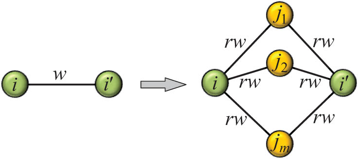
A weighted edge multi-division operation.
With the preparation of the weighted edge multi-division operation, the weighted scale-free networks are constructed in an iterative way as depicted. Let

Illustration for two networks
The iterative growth of the network allows us to precisely analyze its topological characteristics, such as the order and the size, the sum of weights of all edges, and so on. At each time step
The network size
Let symbol
The networks studied in this article display some representative topological characteristics observed in different real-life systems. They obey a significant power-law degree distribution with exponent
Let
then by considering the initial condition
For an edge
where
3 Eigenvalues and their multiplicities of transition weight matrix
In this section, we determine all eigenvalues and multiplicities of transition weight matrix in our networks, according to the relationship between the eigenvalues of the transition weight matrix of two consecutive generations.
3.1 Relationship between eigenvalues
Let
which shows that matrix
For
Let
Given two old nodes
For each element
We know that
For an old node
Comparing equations (13) and (8) corresponding to any old node
furthermore, the solution of
The above result shows that for an eigenvalue
3.2 Multiplicities of eigenvalues
On the basis of the eigenvalues obtained above, we can determine their corresponding multiplicity for matrix
For small networks, we can calculate their eigenvalues and corresponding multiplicities directly, for instance, the set of eigenvalues of
We can observe the fact that in addition to the eigenvalues
In general, we usually use
For the set of all nodes in
where the fact that
Because the matrix
where the first
from which we obtain
In addition, we have
Therefore, we obtain
The total number of eigenvalue 0 and its descendants in
For eigenvalues
Apparently, eigenvalues
which proves that we have found all the eigenvalues, and the corresponding multiplicities of the matrix
4 Applications of eigenvalues
The eigenvalues of the normalized Laplacian matrix of
4.1 Random target access time
We set
The quantity
Equation (27) implies that the random target access time
The normalized Laplacian matrix of
Theorem 1
For
when
Proof
According to equation (15) and
We suppose that
It is easy to obtain the following result due to equation (29):
In order to facilitate calculations, we divide the set
Hence, we still need to evaluate
which indicates that
Combining the above results in equations (30) and (32), the relationship between
Furthermore, using the initial condition
Finally, for large weighted fractal networks, that is
Equation (35) implies that in the large
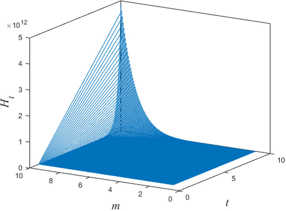
Random target access time
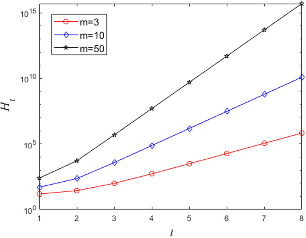
When
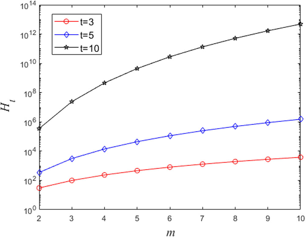
When
4.2 Weighted counting of spanning trees
The spanning tree of a connect network
Different from using the electrical networks theory to obtain the closed-form formula for the spanning tree enumeration [30,31] and calculating the weighted spanning trees through the special structure of the networks [32], in this subsection, we count
Theorem 2
For
Proof
We first need to determine the three terms in equation (36). For the sum term in the denominator, we have
Consider the two product terms in the numerator of equation (36), let
Based on the results of the eigenvalues obtained above, the following equation holds:
Then, multiplying equations (38) by (39) results in
For the simple case of
Inserting the results of two equations (37) and (41) into equation (36), we can obtain the following expression of
The result of equation (42) is consistent with the result of direct enumeration, which verifies that our calculation for the eigenvalues of the transition weight matrix of the weighted network
5 Conclusion
There are many documents that have verified that the weights of some networks have a serious impact on the random target access time. Unlike the existing weighted networks, we have found a family of weighted networks whose random target access time is not controlled by its weight factor, and these networks have been proven to exhibit the remarkable scale-free properties observed in various real-life complex systems. We have listed all eigenvalues for the transition weight matrix of
-
Funding information: This research was supported by the National Key Research and Development Plan under Grant No. 2019YFA0706401 and the National Natural Science Foundation of China under Grant Nos. 61872166 and 61662066, the Technological Innovation Guidance Program of Gansu Province: Soft Science Special Project (21CX1ZA285), and the Northwest China Financial Research Center Project of Lanzhou University of Finance and Economics (JYYZ201905).
-
Author contributions: B.Y. and J.S. created and conceptualized the idea. J.S. wrote the original draft. X.W. and M.Z. reviewed and edited the draft. All authors have accepted responsibility for the entire content of this manuscript and approved its submission. The authors applied the SDC approach for the sequence of authors.
-
Conflict of interest: The authors state no conflict of interest.
-
Data availability statement: Data sharing is not applicable to this article as no datasets were generated or analyzed during this study.
References
[1] X. D. Zhao, R. Tao, X. J. Kang, and W. Li, Hierarchical-biased random walk for urban remote sensing image segmentation, IEEE J. Sel. Top. Appl. Earth Obs. Remote Sens. 12 (2019), no. 5, 1–13, https://doi.org/10.1109/JSTARS.2019.2905352. Search in Google Scholar
[2] M. Bestehorn, A. P. Riascos, T. M. Michelitsch, and B. A. Collet, A Markovian random walk model of epidemic spreading, Continuum Mech. Thermodyn. 33 (2021), no. 10, 1207–1221, https://doi.org/10.1007/s00161-021-00970-z. Search in Google Scholar PubMed PubMed Central
[3] B. F. Hu, H. Wang, and Y. J. Zheng, Sign prediction and community detection in directed signed networks based on random walk theory, Int. J. Emb. Syst. 11 (2019), no. 2, 200, https://doi.org/10.1504/IJES.2019.10019713. Search in Google Scholar
[4] H. Zhang, H. Q. Zhu, and X. F. Ling, Polar coordinate sampling-based segmentation of overlapping cervical cells using attention U-Net and random walk, Neurocomputing 383 (2020), no. 3, 212–223, DOI: https://doi.org/10.1016/j.neucom.2019.12.036. 10.1016/j.neucom.2019.12.036Search in Google Scholar
[5] N. Masuda, M. A. Porter, and R. Lambiotte, Random walks and diffusion on networks, Phys. Rep. 716–717 (2017), 1–58, https://doi.org/10.1016/j.physrep.2017.07.007. Search in Google Scholar
[6] A. P. Riascos and J. L. Mateos, Random walks on weighted networks: a survey of local and non-local dynamics, J. Complex Netw. 9 (2021), 1–39, https://doi.org/10.1093/comnet/cnab032. Search in Google Scholar
[7] M. Levene and G. Loizou, Kemeny’s constant and the random surfer, Amer. Math. Monthly. 109 (2002), no. 8, 741–745, https://doi.org/10.1080/00029890.2002.11919905. Search in Google Scholar
[8] Z. Z. Zhang, A. Julaiti, B. Y. Hou, H. J. Zhang, and G. R. Chen, Mean first-passage time for random walks on undirected network, Eur. Phys. J. B. 84 (2011), no. 4, 691–697, https://doi.org/10.1140/epjb/e2011-20834-1. Search in Google Scholar
[9] E. I. Milovanovi, M. M. Mateji, and I. Z. Milovanovi, On the normalized Laplacian spectral radius, Laplacian incidence energy and Kemeny’s constant, Linear Algebra Appl. 582 (2019), no. 1, 181–196, DOI: https://doi.org/10.1016/j.laa.2019.08.004. 10.1016/j.laa.2019.08.004Search in Google Scholar
[10] P. C. Xie, Z. Z. Zhang, and F. Comellas, On the spectrum of the normalized Laplacian of iterated triangulations of graphs, Appl. Math. Comput. 273 (2016), no. 15, 1123–1129, https://doi.org/10.1016/j.amc.2015.09.057. Search in Google Scholar
[11] Y. F. Chen, M. F. Dai, X. Q. Wang, Y. Sun, and W. Y. Su, Spectral analysis for weighted iterated triangulations of graphs, Fractals 26 (2018), no. 1, 1850017, https://doi.org/10.1142/S0218348X18500172. Search in Google Scholar
[12] L. Gao, J. Peng, C. Tang, and A. P. Riascos, Trapping efficiency of random walks in weighted scale-free trees, J. Stat. Mech. Theory Exp. 2021 (2021), 063405, https://doi.org/10.1088/1742-5468/ac02cb. Search in Google Scholar
[13] M. Liu, Z. Xiong, Y. Ma, P. Zhang, J. Wu, and X. Qi, DPRank centrality: Finding important vertices based on random walks with a new defined transition matrix, Future Gener. Comput. Syst. 83 (2017), 376–389, DOI: https://doi.org/10.1016/j.future.2017.10.036. 10.1016/j.future.2017.10.036Search in Google Scholar
[14] N. Bajorin, T. Chen, A. Dagan, C. Emmons, M. Hussein, M. Khalil, et al., Vibration modes of 3n-gaskets and other fractals, J. Phys. A Math. Theor. 41 (2008), no. 1, 015101, https://doi.org/10.1088/1751-8113/41/1/015101. Search in Google Scholar
[15] A. Julaiti, B. Wu, and Z. Z. Zhang, Eigenvalues of normalized Laplacian matrices of fractal trees and dendrimers: Analytical results and applications, J. Chem. Phys. 138 (2013), no. 20, 204116–204116, https://doi.org/10.1063/1.4807589. Search in Google Scholar PubMed
[16] M. F. Dai, X. Q. Wang, Y. Q. Sun, Y. Sun, and W. Su, Eigentime identities for random walks on a family of treelike networks and polymer networks, Phys. A. 484 (2017), no. 15, 132–140, https://doi.org/10.1016/j.physa.2017.04.172. Search in Google Scholar
[17] A. Irmanova, I. Dolzhikova, and A. P. James, Self tuning stochastic weighted neural networks, IEEE Int. Symp. Circuits Syst. 2020 (2020), 1–5, https://doi.org/10.1109/ISCAS45731.2020.9180809. Search in Google Scholar
[18] A. D. Bona, D. Marcelo, K. O. Fonseca, and R. Luders, A reduced model for complex network analysis of public transportation systems, Phys. A. 567 (2021), 125715, https://doi.org/10.1016/j.physa.2020.125715. Search in Google Scholar
[19] Z. Z. Zhang, X. Y. Guo, and Y. H. Yi, Spectra of weighted scale-free networks, Sci. Rep. 5 (2015), no. 1, 17469, https://doi.org/10.1038/srep17469. Search in Google Scholar PubMed PubMed Central
[20] M. F. Dai, J. Y. Liu, J. W. Chang, D. L. Tang, T. T. Ju, Y. Sun, et al., Eigentime identity of the weighted scale-free triangulation networks for weight-dependent walk, Phys. A. 513 (2019), 202–209, https://doi.org/10.1016/j.physa.2018.08.172. Search in Google Scholar
[21] J. H. Zou, M. F. Dai, X. Q. Wang, H. L. Tang, D. He, Y. Sun, et al., Eigenvalues of transition weight matrix and eigentime identity of weighted network with two hub nodes, Canad. J. Phys. 96 (2017), no. 3, 255–261, DOI: https://doi.org/10.1139/cjp-2017-0274. 10.1139/cjp-2017-0274Search in Google Scholar
[22] E. Q. Zhu, F. Jiang, C. J. Liu, and J. Xu, Partition independent set and reduction-based approach for partition coloring problem, IEEE Trans. Cybern. 52 (2022), no. 6, 1–10, https://doi.org/10.1109/TCYB.2020.3025819. Search in Google Scholar PubMed
[23] C. J. Liu, A note on domination number in maximal outerplanar graphs, Discrete Appl. Math. 293 (2021), no. 1, 90–94, https://doi.org/10.1016/j.dam.2021.01.021. Search in Google Scholar
[24] C. J. Liu, E. Q. Zhu, Y. K. Zhang, Q. Zhang, and X. P. Wei, Characterization, verification and generation of strategies in games with resource constraints, Automatica 140 (2022), 110254, DOI: https://doi.org/10.1016/j.automatica.2022.110254. 10.1016/j.automatica.2022.110254Search in Google Scholar
[25] Z. Z. Zhang, S. G. Zhou, and T. Zou, Self-similarity, small-world, scale-free scaling, disassortativity, and robustness in hierarchical lattices, Eur. Phys. J. B. 56 (2007), no. 3, 259–271, https://doi.org/10.1140/epjb/e2007-00107-6. Search in Google Scholar
[26] H. D. Rozenfeld, S. Havlin, and D. Ben-Avraham, Fractal and transfractal recursive scale-free nets, New J. Phys. 9 (2007), 175, https://doi.org/10.1088/1367-2630/9/6/175. Search in Google Scholar
[27] A. Julaiti, B. Wu, and Z. Z. Zhang, Eigenvalues of normalized Laplacian matrices of fractal trees and dendrimers: Analytical results and applications, J. Chem. Phys. 138 (2013), no. 20, 204116–204116, https://doi.org/10.1063/1.4807589. Search in Google Scholar PubMed
[28] J. G. Kemeny, J. L. Snell, J. G. Kemeny, H. Mirkill, J. L. Snell, G. L. Thompson, et al., Finite Markov chains, Amer. Math. Monthly. 31 (1961), no. 67, 2789587, https://doi.org/10.2307/2309264. Search in Google Scholar
[29] Z. Z. Zhang, S. Q. Wu, M. Y. Li, and F. Comellas, The number and degree distribution of spanning trees in the Tower of Hanoi graph, Theoret. Comput. Sci. 609 (2016), no. 2, 443–455, https://doi.org/10.1016/j.tcs.2015.10.032. Search in Google Scholar
[30] W. G. Sun, S. Wang, and J. Y. Zhang, Counting spanning trees in prism and anti-prism graphs, Appl. Anal. Comput. 6 (2016), no. 1, 65–75, https://doi.org/10.11948/2016006. Search in Google Scholar
[31] Y. L. Shang, On the number of spanning trees, the Laplacian eigenvalues, and the Laplacian Estrada index of subdivided-line graphs, Open Math. 14 (2016), no. 1, 641–648, https://doi.org/10.1515/math-2016-0055. Search in Google Scholar
[32] F. Ma and B. Yao, The number of spanning trees of a class of self-similar fractal models, Inform. Process. Lett. 136 (2018), 64–69, https://doi.org/10.1016/j.ipl.2018.04.004. Search in Google Scholar
© 2022 Jing Su et al., published by De Gruyter
This work is licensed under the Creative Commons Attribution 4.0 International License.
Articles in the same Issue
- Regular Articles
- A random von Neumann theorem for uniformly distributed sequences of partitions
- Note on structural properties of graphs
- Mean-field formulation for mean-variance asset-liability management with cash flow under an uncertain exit time
- The family of random attractors for nonautonomous stochastic higher-order Kirchhoff equations with variable coefficients
- The intersection graph of graded submodules of a graded module
- Isoperimetric and Brunn-Minkowski inequalities for the (p, q)-mixed geominimal surface areas
- On second-order fuzzy discrete population model
- On certain functional equation in prime rings
- General complex Lp projection bodies and complex Lp mixed projection bodies
- Some results on the total proper k-connection number
- The stability with general decay rate of hybrid stochastic fractional differential equations driven by Lévy noise with impulsive effects
- Well posedness of magnetohydrodynamic equations in 3D mixed-norm Lebesgue space
- Strong convergence of a self-adaptive inertial Tseng's extragradient method for pseudomonotone variational inequalities and fixed point problems
- Generic uniqueness of saddle point for two-person zero-sum differential games
- Relational representations of algebraic lattices and their applications
- Explicit construction of mock modular forms from weakly holomorphic Hecke eigenforms
- The equivalent condition of G-asymptotic tracking property and G-Lipschitz tracking property
- Arithmetic convolution sums derived from eta quotients related to divisors of 6
- Dynamical behaviors of a k-order fuzzy difference equation
- The transfer ideal under the action of orthogonal group in modular case
- The multinomial convolution sum of a generalized divisor function
- Extensions of Gronwall-Bellman type integral inequalities with two independent variables
- Unicity of meromorphic functions concerning differences and small functions
- Solutions to problems about potentially Ks,t-bigraphic pair
- Monotonicity of solutions for fractional p-equations with a gradient term
- Data smoothing with applications to edge detection
- An ℋ-tensor-based criteria for testing the positive definiteness of multivariate homogeneous forms
- Characterizations of *-antiderivable mappings on operator algebras
- Initial-boundary value problem of fifth-order Korteweg-de Vries equation posed on half line with nonlinear boundary values
- On a more accurate half-discrete Hilbert-type inequality involving hyperbolic functions
- On split twisted inner derivation triple systems with no restrictions on their 0-root spaces
- Geometry of conformal η-Ricci solitons and conformal η-Ricci almost solitons on paracontact geometry
- Bifurcation and chaos in a discrete predator-prey system of Leslie type with Michaelis-Menten prey harvesting
- A posteriori error estimates of characteristic mixed finite elements for convection-diffusion control problems
- Dynamical analysis of a Lotka Volterra commensalism model with additive Allee effect
- An efficient finite element method based on dimension reduction scheme for a fourth-order Steklov eigenvalue problem
- Connectivity with respect to α-discrete closure operators
- Khasminskii-type theorem for a class of stochastic functional differential equations
- On some new Hermite-Hadamard and Ostrowski type inequalities for s-convex functions in (p, q)-calculus with applications
- New properties for the Ramanujan R-function
- Shooting method in the application of boundary value problems for differential equations with sign-changing weight function
- Ground state solution for some new Kirchhoff-type equations with Hartree-type nonlinearities and critical or supercritical growth
- Existence and uniqueness of solutions for the stochastic Volterra-Levin equation with variable delays
- Ambrosetti-Prodi-type results for a class of difference equations with nonlinearities indefinite in sign
- Research of cooperation strategy of government-enterprise digital transformation based on differential game
- Malmquist-type theorems on some complex differential-difference equations
- Disjoint diskcyclicity of weighted shifts
- Construction of special soliton solutions to the stochastic Riccati equation
- Remarks on the generalized interpolative contractions and some fixed-point theorems with application
- Analysis of a deteriorating system with delayed repair and unreliable repair equipment
- On the critical fractional Schrödinger-Kirchhoff-Poisson equations with electromagnetic fields
- The exact solutions of generalized Davey-Stewartson equations with arbitrary power nonlinearities using the dynamical system and the first integral methods
- Regularity of models associated with Markov jump processes
- Multiplicity solutions for a class of p-Laplacian fractional differential equations via variational methods
- Minimal period problem for second-order Hamiltonian systems with asymptotically linear nonlinearities
- Convergence rate of the modified Levenberg-Marquardt method under Hölderian local error bound
- Non-binary quantum codes from constacyclic codes over 𝔽q[u1, u2,…,uk]/⟨ui3 = ui, uiuj = ujui⟩
- On the general position number of two classes of graphs
- A posteriori regularization method for the two-dimensional inverse heat conduction problem
- Orbital stability and Zhukovskiǐ quasi-stability in impulsive dynamical systems
- Approximations related to the complete p-elliptic integrals
- A note on commutators of strongly singular Calderón-Zygmund operators
- Generalized Munn rings
- Double domination in maximal outerplanar graphs
- Existence and uniqueness of solutions to the norm minimum problem on digraphs
- On the p-integrable trajectories of the nonlinear control system described by the Urysohn-type integral equation
- Robust estimation for varying coefficient partially functional linear regression models based on exponential squared loss function
- Hessian equations of Krylov type on compact Hermitian manifolds
- Class fields generated by coordinates of elliptic curves
- The lattice of (2, 1)-congruences on a left restriction semigroup
- A numerical solution of problem for essentially loaded differential equations with an integro-multipoint condition
- On stochastic accelerated gradient with convergence rate
- Displacement structure of the DMP inverse
- Dependence of eigenvalues of Sturm-Liouville problems on time scales with eigenparameter-dependent boundary conditions
- Existence of positive solutions of discrete third-order three-point BVP with sign-changing Green's function
- Some new fixed point theorems for nonexpansive-type mappings in geodesic spaces
- Generalized 4-connectivity of hierarchical star networks
- Spectra and reticulation of semihoops
- Stein-Weiss inequality for local mixed radial-angular Morrey spaces
- Eigenvalues of transition weight matrix for a family of weighted networks
- A modified Tikhonov regularization for unknown source in space fractional diffusion equation
- Modular forms of half-integral weight on Γ0(4) with few nonvanishing coefficients modulo ℓ
- Some estimates for commutators of bilinear pseudo-differential operators
- Extension of isometries in real Hilbert spaces
- Existence of positive periodic solutions for first-order nonlinear differential equations with multiple time-varying delays
- B-Fredholm elements in primitive C*-algebras
- Unique solvability for an inverse problem of a nonlinear parabolic PDE with nonlocal integral overdetermination condition
- An algebraic semigroup method for discovering maximal frequent itemsets
- Class-preserving Coleman automorphisms of some classes of finite groups
- Exponential stability of traveling waves for a nonlocal dispersal SIR model with delay
- Existence and multiplicity of solutions for second-order Dirichlet problems with nonlinear impulses
- The transitivity of primary conjugacy in regular ω-semigroups
- Stability estimation of some Markov controlled processes
- On nonnil-coherent modules and nonnil-Noetherian modules
- N-Tuples of weighted noncommutative Orlicz space and some geometrical properties
- The dimension-free estimate for the truncated maximal operator
- A human error risk priority number calculation methodology using fuzzy and TOPSIS grey
- Compact mappings and s-mappings at subsets
- The structural properties of the Gompertz-two-parameter-Lindley distribution and associated inference
- A monotone iteration for a nonlinear Euler-Bernoulli beam equation with indefinite weight and Neumann boundary conditions
- Delta waves of the isentropic relativistic Euler system coupled with an advection equation for Chaplygin gas
- Multiplicity and minimality of periodic solutions to fourth-order super-quadratic difference systems
- On the reciprocal sum of the fourth power of Fibonacci numbers
- Averaging principle for two-time-scale stochastic differential equations with correlated noise
- Phragmén-Lindelöf alternative results and structural stability for Brinkman fluid in porous media in a semi-infinite cylinder
- Study on r-truncated degenerate Stirling numbers of the second kind
- On 7-valent symmetric graphs of order 2pq and 11-valent symmetric graphs of order 4pq
- Some new characterizations of finite p-nilpotent groups
- A Billingsley type theorem for Bowen topological entropy of nonautonomous dynamical systems
- F4 and PSp (8, ℂ)-Higgs pairs understood as fixed points of the moduli space of E6-Higgs bundles over a compact Riemann surface
- On modules related to McCoy modules
- On generalized extragradient implicit method for systems of variational inequalities with constraints of variational inclusion and fixed point problems
- Solvability for a nonlocal dispersal model governed by time and space integrals
- Finite groups whose maximal subgroups of even order are MSN-groups
- Symmetric results of a Hénon-type elliptic system with coupled linear part
- On the connection between Sp-almost periodic functions defined on time scales and ℝ
- On a class of Harada rings
- On regular subgroup functors of finite groups
- Fast iterative solutions of Riccati and Lyapunov equations
- Weak measure expansivity of C2 dynamics
- Admissible congruences on type B semigroups
- Generalized fractional Hermite-Hadamard type inclusions for co-ordinated convex interval-valued functions
- Inverse eigenvalue problems for rank one perturbations of the Sturm-Liouville operator
- Data transmission mechanism of vehicle networking based on fuzzy comprehensive evaluation
- Dual uniformities in function spaces over uniform continuity
- Review Article
- On Hahn-Banach theorem and some of its applications
- Rapid Communication
- Discussion of foundation of mathematics and quantum theory
- Special Issue on Boundary Value Problems and their Applications on Biosciences and Engineering (Part II)
- A study of minimax shrinkage estimators dominating the James-Stein estimator under the balanced loss function
- Representations by degenerate Daehee polynomials
- Multilevel MC method for weak approximation of stochastic differential equation with the exact coupling scheme
- Multiple periodic solutions for discrete boundary value problem involving the mean curvature operator
- Special Issue on Evolution Equations, Theory and Applications (Part II)
- Coupled measure of noncompactness and functional integral equations
- Existence results for neutral evolution equations with nonlocal conditions and delay via fractional operator
- Global weak solution of 3D-NSE with exponential damping
- Special Issue on Fractional Problems with Variable-Order or Variable Exponents (Part I)
- Ground state solutions of nonlinear Schrödinger equations involving the fractional p-Laplacian and potential wells
- A class of p1(x, ⋅) & p2(x, ⋅)-fractional Kirchhoff-type problem with variable s(x, ⋅)-order and without the Ambrosetti-Rabinowitz condition in ℝN
- Jensen-type inequalities for m-convex functions
- Special Issue on Problems, Methods and Applications of Nonlinear Analysis (Part III)
- The influence of the noise on the exact solutions of a Kuramoto-Sivashinsky equation
- Basic inequalities for statistical submanifolds in Golden-like statistical manifolds
- Global existence and blow up of the solution for nonlinear Klein-Gordon equation with variable coefficient nonlinear source term
- Hopf bifurcation and Turing instability in a diffusive predator-prey model with hunting cooperation
- Efficient fixed-point iteration for generalized nonexpansive mappings and its stability in Banach spaces