Mathematical model for conversion of groundwater flow from confined to unconfined aquifers with power law processes

Makosha Ishmaeline Charlotte Morakaladi; Abdon Atangana

doi:10.1515/geo-2022-0446

Article Open Access

Mathematical model for conversion of groundwater flow from confined to unconfined aquifers with power law processes

Makosha Ishmaeline Charlotte Morakaladi and Abdon Atangana

Published/Copyright: March 15, 2023

Published by

Become an author with De Gruyter Brill

Submit Manuscript Author Information

From the journal Open Geosciences Volume 15 Issue 1

Abstract

In this work, we propose a mathematical model to depict the conversion of groundwater flow from confined to unconfined aquifers. The conversion problem occurs due to the heavy pumping of confined aquifers over time, which later leads to the depletion of an aquifer system. The phenomenon is an interesting one, hence several models have been developed and used to capture the process. However, one can point out that the model has limitations of its own, as it cannot capture the effect of fractures that exist in the aquitard. Therefore, we suggest a mathematical model where the classical differential operator that is based on the rate of change is substituted by a non-conventional one including the differential operator that can represent processes following the power law to capture the memory effect. Moreover, we revise the properties of the aquitard to evaluate and capture the behaviors of flow during the process in a different aquitard setting. Numerical analysis was performed on the new mathematical models and numerical solutions were obtained, as well as simulations for various fractional order values.

Keywords: confined aquifer; unconfined aquifer; aquitard; differential operator; rate of change; power law

1 Introduction

An aquitard is found to be a distinctive hydrogeological system that has low permeability to store sufficient groundwater supply but can store a significant amount of groundwater supply [1,2]. These formations are often ignored as sources of groundwater supply as they are assumed to be homogeneous and cover a large area to an extent where they are mischaracterized to restrict flow from one aquifer to another [2,3]. An aquitard can store and transmit groundwater to an aquifer in various ways including through fractures and pumping [4]. The amount of groundwater storage depends on the density of the fractures [5].

Modeling groundwater movement within geological formations seems to be a challenging issue since one cannot see how the flow occurs within the aquifer. Mathematical models were developed to depict physical problems such as the conversion of flow, it can, however, be pointed out that some heterogeneities of a geological formation are not considered. Complexities in nature exist such as the flow of water taking place in a fracture, which is now considered in mathematical models. It is known that the distribution of fractures controls the flow distribution and propagation within naturally fractured reservoirs [6]. The existence of fractures in a formation at various degrees creates a level of uncertainty and heterogeneity in the construction of a mathematical model [7].

Mathematical models have been suggested in the past to model the conversion of flow and have been used by many researchers over the years [8,9,10,11,12,13]. The models were developed to capture the conversion based on one type of aquitard setting and used differential and integral operators based on the concept of rate of change. Even though these operators have been utilized successfully in many disciplines, researchers discovered that they could only be used to represent classical mechanical problems with no memory [14]. As a result, there was a pressing urge to develop novel mathematical techniques that could be utilized to portray non-conventional behavior, as several problems remained unsolvable. In particular, the movement of groundwater within a geological formation with a fracture network is governed by the power law process [15,16,17,18,19]. It has been taken into account in several studies due to its capacity to describe moving objects in a single medium and its long-range memory [20].

A study done by Xiao et al. [21] proved that the existing numerical solutions that were developed for transient confined to unconfined flow have insufficient analyses of the dissimilarities in hydraulic properties found between the confined and unconfined areas. The analytical solution developed by Moench and Prickett [13] does not consider differences in transmissivity and the recently developed analytical solution by Hu and Chen [22] neglects differences in diffusivity [23]. In this study, we evaluate the differences in the aquitard settings of the existing model and the suggested model that comprises fractures for the transfer of flow during the conversion process.

Recently it has been studied by Tateishi et al. [23] how fractional operators can modify the behavior of waiting time distribution. In this study, we introduce a fractional operator that will capture the transfer of flow in the aquitard when water passes through fractures and evaluate the waiting time distribution yields of the suggested model as compared to the previously suggested models. The fractional operator is essential in diffusion as it displays the inherent regularities in a system’s features and is widely considered to model nature and its complexities. Due to its significance in modeling complex situations, we apply the Caputo fractional derivative [24] to the classical confined-to-unconfined flow equation to develop a new model.

2 Background of the existing model for confined and unconfined aquifers

Given that the aquifer is confined, homogeneous, and infinite, the Theis solution [25] for the confined flow is developed using a numerical solution with the associated initial and boundary of a two-dimensional liquid flow propagating radially from or to an origin. This is an analytical method for confined transient flow in an abstraction well using a connection between the conduction of heat and transitory groundwater flow [26], and is expressed as follows:

(1) ∂ 2 h ∂ r 2 + 1 r ∂ h ∂ r = S T ∂ h ∂ t ,

where h = hydraulic head, r = radial distance from the well, S = storage coefficient, T = transmissivity, and t = time since pumping started.

Due to the non-linearity of unconfined aquifers, Boulton [27] expanded Theis’ transient confined theory to incorporate the influence of water table in those aquifers, given as follows:

(2) S / T ∂ h ∂ t = ∂ h r ∂ r + ∂ 2 h ∂ r 2 − α S y ∫ 0 t ∂ h ∂ τ exp [ − α ( t − τ ) ] d τ ,

where S _y = specific yield of the unconfined aquifer, α = the empirical constant, a reciprocal of the delay index in minutes − 1 , and e − α ( t − τ ) = delay index.

In this study, the confined to unconfined flow model is represented by a system of equations. equation (1) represents the flow in a confined aquifer, which was proposed by Theis and the equation (2) is an integrodifferential partial differential equation that represents the flow in an unconfined aquifer suggested by Boulton. Therefore, the confined to unconfined flow is represented by the following systems of equations, respectively:

(3) S c T ∂ h ∂ t = 1 r ∂ h ∂ r + ∂ 2 h ∂ r 2 , h ≥ B S T ∂ h ∂ t = 1 r ∂ h ∂ r + ∂ 2 h ∂ r 2 − α S y ∫ 0 t ∂ h ∂ τ exp [ − α ( t − τ ) d τ ] , 0 < h ≤ B .

The aforementioned delay is unmistakably a representation of fractional differential operators with an exponential decay law process, which take fading memory or decay behaviors into account. However, it is important to note that many processes, which will be covered in more detail in the following sections, can be seen.

3 Conceptual model

Many researchers have pointed out that fractional derivatives that are developed upon the power law, t − α , are powerful mathematical tools used to accurately detail flow in elastic media [28,29]. The power law has successfully been used to model what happens in nature together with its complexities; therefore, the power law is strongly preferred in diffusion problems to reveal regularities that occur in a system [30]. Fractional differential operators have been used over the past years to simulate real-world physical problems that often lead to a waiting time distribution that is guided by the power law [31]. A typical property of the power law is that it shows a scale-invariance, this can be described as a characteristic of laws or objects that cannot transform even when the scale of length or other variables are multiplied by a common factor, thereby showing universality [32,33,34,35]. The mean square displacement (MSD) in this case is practical as it can develop a model that can depict flow in a closed system. This property can estimate the evolution of a particle’s position with respect to time and can reveal whether a particle’s spreading is mostly caused by advection or diffusion [36].

The power law function can be used with great success to model the complex nature of the real world, hence for this study we use this powerful mathematical tool to simulate the conversion of flow. Due to the presence of fractures, we use the differential operator that is based upon the power law kernel and has MSD properties. The aquitard of the model consists of some fractures, which correspond to the power law and will be captured using a fractional derivative operator depicting the fading memory process. The conceptual model depicts groundwater flow from a confining layer to an unconfined unit to the surface of the earth, by seeping through a natural formation such as fractures through an aquitard. We assume that there is a passage within the geological formation where the crossover takes place, for this study, the passage is referred to as a geological formation known as an aquitard. The aquitard in the model is a fractured crystalline rock that lies adjacent to the aquifer. The crystalline rock in the model is an intrusive rock known as granite that consists of a few fractures. Granite is an igneous rock that is very hard and dense, granular crystalline igneous rock that is commonly comprised of quartz, feldspar, and mica [37]. The formation has a lower hydraulic conductivity which can store water but can slowly transmit water as it partially restricts flow. The presence of fractures provides a flow path for water to seep and percolate deep underneath to form a groundwater aquifer. Granite is composed of crystals formed by the chilling of magma with a certain silica content and is frequently detected below within the earth’s crust [38,39,40]. This magma moves to a location where it cools slowly and solidifies without reaching the earth’s surface and forms interlocking crystals [41]. Granite generally has the property that as the magma cools, the crystals get bigger, and as they cool more quickly, the crystals become smaller [42,43]. The fractures in the formation in the conceptual model were developed due to the extreme variation in weather conditions that cause shrinkage. The network of fractures provides a low-permeable conduit that feeds water to the pumping well.

The conceptual model presented is compared with the existing model, the Moench and Prickett model [13] (Figure 1), where the following assumptions are similar: consider a confined aquifer that covers a wider area horizontally with a horizontal initial piezometric head, h . The confined layer is completely penetrated by a pumping well and discharges at a constant rate, Q . The pumping well in the aquifer generates the transient flow. When the groundwater level falls below the upper border of the confined aquifer, the piezometric surface continues to fall below the overlying aquitard, forming an unconfined zone in the region of the well. With continuous pumping, the hydraulic head in the pumping well, h , drops below the top of the confined aquifer, 0 < h ≤ B , where B is the confined unit’s thickness. An area with a radial distance less than the spacing of the transient confined to an unconfined point from the abstraction well immediately becomes unconfined, where r is the radial distance from the pumping well [12,44].

$Figure 1 Schematic illustration of confined to unconfined flow toward a completely penetrated well passing through an overlying aquitard (fractured granite) in a confined aquifer [44].$

Figure 1

Schematic illustration of confined to unconfined flow toward a completely penetrated well passing through an overlying aquitard (fractured granite) in a confined aquifer [44].

4 The power law kernel

Some mathematical functions have characteristics that are similar to those found in nature. According to one of these, the power law function, a change in one variable with respect to another will cause a change in the other quantity that is commensurate to that change. The differentiation and integration topics used this power law function as a kernel.

(4) K ( α , t ) = t − α Γ ( 1 − α ) .

The power law as a function of time and alpha is graphically depicted in Figure 2.

Figure 2

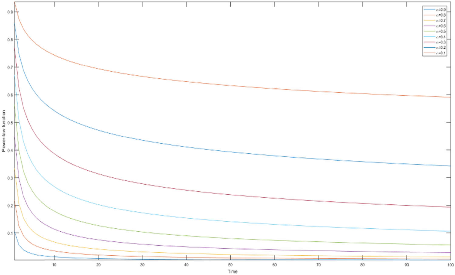
Numerical representation of the power law function for different orders.

Power law is scale invariant, as can be seen from the preceding graphic, which is completely consistent with the arguments made by several published materials. The Laplace transform of this function is given as follows:

(5) L t − α Γ ( 1 − α ) = s α − 1 .

The Bode diagram and the phase diagram can then be examined to determine which process this expression might result in when used to signal analysis (Figures 3 and 4).

Figure 3

Bode and phase diagram for the Laplace transform of power law.

Figure 4

Bode and phase diagram for power law.

The power law is scale invariant even in Laplace space, as demonstrated by the accompanying Bode diagrams and phases diagrams. However, the long-tailed power law property can be included in the flow of a single fracture in the context of geohydrology. A feature that can be used to illustrate flow through an aquitard, where an aquifer changes from being confined to unconfined with a single fracture. In the context of fractional calculus, a differential operator based on the power law was introduced, which will be presented below.

The Riemann–Liouville (R–L) fractional derivative is a local operator with a singular memory kernel that is developed upon using the power law kernel [45]. The definition of the R–L fractional derivative is as follows:

(6) D x α ( f ( x ) ) = d n d x n D x − ( n − α ) ( f ( x ) ) = d n d x n I x n − α ( f ( x ) ) ,

(7) D b α ( f ( x ) ) = d n d x n D b − ( n − α ) ( f ( x ) ) = d n d x n I b n − α ( f ( x ) ) ,

where α is a fractional order, however, a base point.

The Caputo derivative [24] is given as follows:

(8) D x α 0 C ( f ( x ) ) = 1 Γ ( n − α ) ∫ 0 x ( x − t ) n − α − 1 d n f ( t ) d t n d t , n − 1 < α ≤ n .

where Γ ( . ) is the Euler gamma function. Caputo also proposed another fractional derivative that is developed upon the power law in 1967 [24].

5 Waiting time distribution

The waiting time is considered in many complex situations in numerous fields of science and engineering. The analysis of waiting times till the actual event happens is a crucial statistical problem studied by researchers in these disciplines. Pareto or gamma distributions are two common models that have been established for the waiting and non-waiting times, respectively [46]. Gamma distributions are characterized by short tails for the waiting time to be kept short and heavy tails for the non-waiting time to be kept long in Pareto distributions [47]. There are many uses for the waiting time distribution; however, it is important to note that there is no unique formula for computing this distribution [48]. Most applications have waiting times that follow a power law behavior [49,50]. The waiting times for examination or between examinations that are higher than the specified threshold is heavy-tailed for a particular usage. When the waiting times have probability tails with variable lengths that approximate a power law, the mean and variance of the waiting times can both be infinite [51]. Over the years, this principle has been applied to characterize diffusion processes with success, and the analytical form of the distribution of waiting times is given as

ω ( t ) ,

where this is known as the “sojourn times” in a case where a diffusing particle temporarily stays at a specific place or velocity. Recently developed more efficient algorithms for power law waiting time distributions have made it easier to study such physical problems with power law random walks and to assess the empirical data.

In terms of the fractional operator of the R–L, the waiting time distribution is given as follows:

ω ( t ) = 1 τ c t α − 1 E α , α − 1 τ c t α ,

where E _α,_α (.) represents the generalized Mittag-Leffler function that has an asymptotic behavior that is expressed by a power law ω ( t ) ∼ 1 / t α − 1 for t → ∞ [23]. Figure 5 presents the waiting time distribution for different values of fractional orders.

$Figure 5 Graphical representation of waiting time for different values of fractional order.$

Figure 5

Graphical representation of waiting time for different values of fractional order.

For comparison sake, we also present the waiting time distribution for the exponential decay kernel used in equation (3). The formula for the waiting time distribution in the case of exponential function is given as follows:

ω ( t ) = 1 τ c exp − 1 τ c t ,

which is a special case of the generalized Mittag-Leffler function when the fractional order is 1. Figure 6 presents the graphical representation of the waiting time distribution associated with the exponential function.

Figure 6

Waiting time distribution for exponential kernel.

In this work, we, therefore, modify the existing equation with the following:

(9) D t α 0 C h ( r , t ) = T S c 1 r ∂ h ( r , t ) ∂ r + ∂ 2 h ( r , t ) ∂ r 2 , h > B ∂ h ( r , t ) ∂ r = T S 1 r ∂ h ∂ r + ∂ 2 h ∂ r 2 − a S y Γ ( 1 − α ) ∫ t 0 ∂ h ( r , τ ) ∂ τ ( t − τ ) − α d τ , h < B .

In the above, the decay process with exponential kernel is replaced by the decay process with the power law kernel.

6 Numerical analysis of confined to unconfined aquifer flow by applying the Caputo fractional operator

In this subsection, the Caputo fractional derivative is used on the classical system of equations that represent the confined to unconfined flow. The discretization of the Caputo fractional derivative is as follows:

(10) D t α 0 C h ( t ) = 1 Γ ( 1 − α ) ∫ 0 t h ′ ( τ ) ( t − τ ) − α d τ .

At t = t n + 1 , employing the numerical approximation of the first derivative, equation (10) gives:

(11) D t n + 1 α 0 C h ( t ) = 1 Γ ( 1 − α ) ∫ 0 t n + 1 h ′ ( τ ) ( t n + 1 − τ ) − α d τ ,

(12) D t n + 1 α 0 C h ( t ) = 1 Γ ( 1 − α ) ∑ j = 0 n h ( t j + 1 ) − h ( t j ) ∆ t ∫ t j t j + 1 ( t n + 1 − τ ) − α d τ ,

(13) D t n + 1 α 0 C h ( t ) = 1 Γ ( 1 − α ) ∑ j = 0 n h ( t j + 1 ) − h ( t j ) ∆ t ∫ t j t j + 1 ( t n + 1 − τ ) − α d τ .

Integrating

(14) D t n + 1 α 0 C h ( t ) = 1 Γ ( 1 − α ) ∑ j = 0 n h ( t j + 1 ) − h ( t j ) ∆ t ∫ t n + 1 − t j t n + 1 − t j + 1 ( y ) − α ( − d y ) ,

(15) D t n + 1 α 0 C h ( t ) = 1 Γ ( 1 − α ) ∑ j = 0 n h ( t j + 1 ) − h ( t j ) ∆ t ( t n + 1 − t j ) 1 − α 1 − α − ( t n + 1 − t j + 1 ) 1 − α 1 − α .

Finally, we obtain

(16) D t n + 1 α 0 C h ( t ) = ( ∆ t ) − α Γ ( 2 − α ) ∑ j = 0 n ( h ( t j + 1 ) − h ( t j ) ) { ( n + 1 − j ) 1 − α − ( n − j ) 1 − α } .

This completes the discretization of the Caputo fractional derivative, which can be found in some already published materials for the sake of geo-hydrologist. Also, the above will be used below for a straightforward method.

6.1 Numerical solution for the model with a straightforward method

Considering the unconfined aquifer equation and replacing the power law kernel in the equation solution gives the following:

(17) S T ∂ h ( r , t ) ∂ t = 1 r ∂ h ( r , t ) ∂ r + ∂ 2 h ( r , t ) ∂ r 2 − α S y ∫ 0 t ∂ h ( r , τ ) ∂ τ ( t − τ ) − α Γ ( 1 − α ) d τ .

Using the numerical approximation equation (16), while taking into consideration the model under review for unconfined aquifers which is given by

(18) S T ∂ h ( r , t ) ∂ t = 1 r ∂ h ( r , t ) ∂ t + ∂ 2 h ( r , t ) ∂ r 2 − α S y ∫ 0 t h ′ ( r , τ ) [ ( t − τ ) ] d τ .

Thereby, the following numerical solution is derived:

(19) S T h ( r i , t j + 1 ) − h ( r i , t j ) ∆ t = 1 r i h i + 1 n − h i − 1 n 2 ∆ r + h i + 1 n − 2 h i n + h i − 1 n ∆ r 2 − ( ∆ t ) − α Γ ( 2 − α ) α S y ∑ j = 0 n h ( r i , t j + 1 ) − h ( r i , t j ) { ( n + 1 − j ) 1 − α − ( n − j ) 1 − α } ,

which gives the numerical solution of the unconfined aquifer of the system analyzed using the Caputo fractional derivative. For the confined part, we have

(20) ( ∆ t ) − α Γ ( 2 − α ) ∑ j = 0 n ( h ( r i , t j + 1 ) − h ( r i , t j ) ) { ( n + 1 − j ) 1 − α − ( n − j ) 1 − α } = 1 r i h i + 1 n − h i − 1 n 2 ∆ r + h i + 1 n − 2 h i n + h i − 1 n ∆ r 2 .

6.2 Numerical solution of the confined aquifer by using Lagrange polynomial

The Lagrange polynomial is used to numerically solve the equation with the Caputo fractional derivative. In the study of numerical analysis, the Lagrange polynomials are generally applied for polynomial interpolation [52], which is the interpolation of a certain set of data by the polynomial of the smallest degree that passes through the points of the dataset. Interpolation is defined as a technique for approximating the value of the dependent variable corresponding to a value of the independent variable falling among its two extreme values based on the supplied values of the independent and dependent variables [53].

(21) S T D t α 0 c h ( r , t ) = ∂ h ( r , t ) r ∂ r + ∂ 2 h ( r , t ) ∂ r 2 ,

(22) D t α 0 c h ( r , t ) = T S ∂ h ( r , t ) r ∂ r + ∂ 2 h ( r , t ) ∂ r 2 ,

(23) T S ∂ h ( r , t ) r ∂ r + ∂ 2 h ( r , t ) ∂ r 2 = f ( r , t , h ( r , t ) ) ,

(24) h ( r , t ) − h ( r , 0 ) = 1 Γ ( α ) ∫ 0 t f ( r , τ , h ( r , τ ) ) ( t − τ ) α − 1 d τ .

Considering ( r i , t n + 1 )

(25) h ( r i , t n + 1 ) − h ( r i , 0 ) = 1 Γ ( α ) ∫ 0 t n + 1 f ( r i , τ , h ( r i , τ ) ) ( t n + 1 − τ ) α − 1 d τ .

Now

(26) h i n + 1 − h i 0 = 1 Γ ( α ) ∑ j = 0 n ∫ t j t j + 1 f ( r i , τ , h ( r i , τ ) ) ( t n + 1 − τ ) α − 1 d τ .

Approximating f ( r i , τ , h ( r i , τ ) ) = P j ( τ ) at ( t j − 1 , t j + 1 )

(27) P j ( τ ) = τ − t j − 1 t j − t j − 1 f ( r i , τ , h i j ) + τ − t j t j − 1 − t j f ( r i , τ , h i j − 1 ) .

Thus

(28) h i n + 1 − h i 0 = 1 Γ ( α ) ∑ j = 0 n ∫ t j t j + 1 τ − t j − 1 ∆ t f ( r i , τ , h i j ) + τ − t j ∆ t f ( r i , τ , h i j − 1 ) ( t n + 1 − τ ) α − 1 d τ .

Therefore, using the integral, the following is obtained:

(29) h i n + 1 − h i 0 = ∑ j = 0 n ( ∆ t ) α Γ ( α + 2 ) f ( r i , t j , h i j ) { ( n + 1 − j ) α ( n − j + 2 + α ) − ( n − j ) α ( n − j + 2 + 2 α ) } − ( ∆ t ) α Γ ( α + 2 ) f ( r i , t j − 1 , h i j − 1 ) { ( n + 1 − j ) α + 1 − ( n − j ) α ( n − j + 1 + α ) } ,

where

(30) f ( r i , t j , h i j ) = T S 1 r i h i + 1 j − h i − 1 j 2 ∆ r + h i + 1 j − 2 h i j + h i − 1 j ( ∆ r ) 2 ,

(31) f ( r i , t j − 1 , h i j − 1 ) = T S 1 r i h i + 1 j − 1 − h i − 1 j − 1 2 ∆ r + h i + 1 j − 1 − 2 h i j − 1 + h i − 1 j − 1 ( ∆ r ) 2 .

Using the numerical approximation equation (29) and recalling the model under investigation for confined aquifers given as follows:

(32) S T D t α 0 c h ( r , t ) = ∂ h ( r , t ) r ∂ r + ∂ 2 h ( r , t ) ∂ r 2 ,

we obtain the following numerical solution:

(33) h i n + 1 − h i 0 = ∑ j = 0 n ( ∆ t ) α Γ ( α + 2 ) T S 1 r i h i + 1 j − h i − 1 j 2 ∆ r + h i + 1 j − 2 h i j + h i − 1 j ( ∆ r ) 2 { ( n − j + 1 ) α ( n − j + 2 + α ) − ( n − j + 2 + 2 α ) ( n − j ) α } − ( ∆ t ) α Γ ( α + 2 ) T S 1 r i h i + 1 j − 1 − h i − 1 j − 1 2 ∆ r + h i + 1 j − 1 − 2 h i j − 1 + h i − 1 j − 1 ( ∆ r ) 2 { ( n − j + 1 ) α + 1 − ( n − j ) α ( n − j + 1 + α ) } ,

which is the numerical solution of the governing confined aquifer equation obtained using Caputo fractional derivative using the Lagrange Polynomial method.

7 Numerical method with piecewise interpolation and Newton polynomial

Many scholars have turned their focus to numerical analysis since the concept of linear interpolation was first presented years ago. Some of the key proposed techniques are the Euler method, Gaussian elimination, Lagrange interpolation polynomial, or Newton’s method [54]. In academics, there are several numerical methods for solving ordinary differential equations, especially nonlinear cases. The well-known Adams–Bashforth method, which is based on the renowned Lagrange interpolation polynomial, is possibly one of the most well-known strategies. Nevertheless, as shown in several published works, the Lagrange polynomial is not as efficient as the Newton polynomial method. As a result, the new numerical method developed by Atangana and Araz [55] is proposed in this subsection. This method, known as piecewise modeling and based on Newton’s interpolation polynomial, can solve fractional and fractal-fractional differential equations. Alternatively, the following numerical schemes can be used to derive the solution to the system.

We consider first a general partial differential equation.

(34) D t α 0 C u ( x , t ) = f ( x , t , u ( x , t ) ) , u ( x , 0 ) = g ( x ) , u ( 0 , t ) = l ( t ) .

We assume that the function f ( x , t , u ( x , t ) ) is two times differentiable with respect to the variable t and n times differentiable with respect to the variable x .

We assume that 0 < x < L and 0 < t < T and

we consider that ∆ x = x i + 1 − x i and ∆ t = t j + 1 − t j .

We fixed x = x i and have

(35) D t α 0 C u ( x i , t ) = f ( x i , t , u ( x i , t ) )

Then applying the R–L integral on both sides, we obtain

(36) u ( x i , t ) = u ( x i , 0 ) + 1 Γ ( α ) ∫ 0 t ( t − τ ) α − 1 f ( x i , τ , u ( x i , τ ) ) d τ .

At t n + 1 = t , we have

(37) u ( x i , t n + 1 ) = u ( x i , 0 ) + 1 Γ ( α ) ∑ j = 0 n ∫ t j t j + 1 ( t n + 1 − τ ) α − 1 × f ( x i , τ , u ( x i , τ ) ) d τ .

Approximating the function f ( x i , τ , u ( x i , τ ) ) by the piecewise interpolation polynomial, one yields the following:

(38) u ( x i , t n + 1 ) = u ( x i , 0 ) + ( ∆ t ) α Γ ( α + 2 ) ∑ j = 0 n ɤ j , n + 1 α f ( x i , t j , u ( x i , t j ) ) + ɤ n + 1 , n + 1 f ( x i , t n + 1 , u p ( x i , t n + 1 ) ) ,

where the coefficients were given follows:

(39) ɤ j , n + 1 α = n α + 1 − ( n − α ) ( n + 1 ) α , j = 0 , ( n − j + 2 ) α + 1 − 2 ( n − j + 1 ) α + 1 − ( n − j ) α + 1 , if 1 ≤ j ≤ n , 1 , if j = n + 1 ,

where

(40) u n + 1 p = u ( x i , 0 ) + 1 Γ ( α ) ∫ 0 t n + 1 ( t n + 1 − τ ) α − 1 f ( x i , τ , u ( x i , τ ) ) d τ ,

(41) = u ( x i , 0 ) + 1 Γ ( α ) ∑ j = 0 n ∫ 0 t n + 1 ( t n + 1 − τ ) α − 1 f ( x i , τ , u ( x i , τ ) ) d τ ,

(42) = u ( x i , 0 ) + ( ∆ t ) α Γ ( α + 1 ) ∑ j = 0 n f ( x i , t j , u ( x i , t j ) ) × { ( n − j + 1 ) α − ( n − j ) α } ,

(43) u n + 1 p = u i 0 + ( ∆ t ) α Γ ( α + 1 ) ∑ j = 0 n f ( x i , t j , u ( x i , t j ) ) { ( n − j + 1 ) α − ( n − j ) α } ,

(44) ɤ n + 1 , n + 1 = 1 .

Or the function can be approximated using the Newton polynomial interpolation to obtain:

(45) u ( x i , t n + 1 ) − u ( x i , 0 ) = ( ∆ t ) α Γ ( α + 1 ) ∑ j = 2 n f ( x i , t j − 2 , u ( x i , t j − 2 ) ) { ( n − j + 1 ) α − ( n − 1 ) α } + ( ∆ t ) α Γ ( α + 2 ) ∑ j = 2 n [ f ( x i , t j − 1 , u ( x i , t j − 1 ) ) − f ( x i , t j − 2 , u ( x i , t j − 2 ) ) ] { ( n − j + 1 ) α ( n − j + 3 + 2 α ) − ( n − j ) α ( n − j + 3 + 3 α ) } + ( ∆ t ) α 2 Γ ( α + 3 ) ∑ j = 2 n ( f ( x i , t j , u ( x i , t j ) ) − 2 f ( x i , t j − 1 , u ( x i , t j − 1 ) ) + f ( x i , t j − 2 , u ( x i , t j − 2 ) ) ) { ( n − j + 1 ) α ( 2 ( n − j ) 2 + ( 3 α + 10 ) ( n − j ) + ( 2 α 2 + 9 α + 12 ) ) − ( n − j ) α ( 2 ( n − j ) 2 + ( 5 α + 10 ) ( n − j ) + ( 6 α 2 + 18 α + 12 ) ) } .

We apply these techniques to our equations. For the confined part, we have the following:

(46) D t α 0 C h ( r , t ) = T S c 1 r ∂ h ( r , t ) ∂ r + ∂ 2 h ( r , t ) ∂ r 2 , h < B , ∂ h ( r , t ) ∂ r = T S 1 r ∂ h ∂ r + ∂ 2 h ∂ r 2 − a S y Γ ( 1 − α ) ∫ t 0 ∂ h ( r , τ ) ∂ τ ( t − τ ) − α d τ , h < B ,

(47) D t α 0 C h ( r , t ) = F 1 ( r , t , h ( r , t ) ) , if h > B , ∂ h ( r , t ) ∂ r = F 2 ( r , t , h ( r , t ) ) , if h < B ,

(48) h ( r , t ) − h ( r , 0 ) = 1 Γ ( α ) ∫ 0 t F 1 ( r , τ , h ( r , τ ) ) ( t − τ ) α − 1 d τ , if h > B h ( r , t ) − h ( r , 0 ) = ∫ 0 t F 2 ( r , τ , h ( r , τ ) ) d τ , if h < B

Applying the suggested routine yields the following:

(49) h ( r i , t n + 1 ) = h ( r i , 0 ) + ( ∆ t ) α Γ ( α + 1 ) ∑ j = 2 n T S c 1 r i h ( r i + 1 , t j − 2 ) − h ( r i − 1 , t j − 2 ) 2 ∆ r + h ( r i + 1 , t j − 2 ) − 2 h ( r i , t j − 2 ) + h ( r i − 1 , t j − 2 ) ∆ r 2 + ( ∆ t ) α Γ ( α + 2 ) ∑ j = 2 n T S c 1 r i h ( r i + 1 , t j − 1 ) − h ( r i − 1 , t j − 1 ) 2 ∆ r + h ( r i + 1 , t j − 1 ) − 2 h ( r i , t j − 1 ) + h ( r i − 1 , t j − 1 ) ∆ r 2 − T S c 1 r i h ( r i + 1 , t j − 2 ) − h ( r i − 1 , t j − 2 ) 2 ∆ r + h ( r i + 1 , t j − 2 ) − 2 h ( r i , t j − 2 ) + h ( r i − 1 , t j − 2 ) ∆ r 2 + ( ∆ t ) α 2 Γ ( α + 3 ) ∑ j = 2 n T S c 1 r i h ( r i + 1 , t j ) − h ( r i − 1 , t j ) 2 ∆ r + h ( r i + 1 , t j ) − 2 h ( r i , t j ) + h ( r i − 1 , t j ) ∆ r 2 − 2 1 r i h ( r i + 1 , t j − 1 ) − h ( r i − 1 , t j − 1 ) 2 ∆ r + h ( r i + 1 , t j − 1 ) − 2 h ( r i , t j − 1 ) + h ( r i − 1 , t j − 1 ) ∆ r 2 + 1 r i h ( r i + 1 , t j − 2 ) − h ( r i + 1 , t j − 2 ) 2 ∆ r + h ( r i + 1 , t j − 2 ) − 2 h ( r i , t j − 2 ) + h ( r i − 1 , t j − 2 ) ∆ r 2 × { ( n − j + 1 ) α ( 2 ( n − j ) 2 + ( 3 α + 10 ) ( n − j ) + ( 2 α 2 + 9 α + 12 ) ) − ( n − j ) α ( 2 ( n − j ) 2 + ( 5 α + 10 ) ( n − j ) + ( 6 α 2 + 18 α + 12 ) ) } , if h > B .

But when h < B , we have the following:

(50) h ( r i , t n + 1 ) = h ( r i , t n ) + 3 2 ∆ t F 2 ( r i , t n , h ( r i , t n ) ) − ∆ t 2 F 2 ( r i , t n − 1 , h ( r i , t n − 1 ) ) ,

where

(51) F ( r i , t n , h ( r i , t n ) ) = 1 r i h ( r i + 1 , t n ) − h ( r i − 1 , t n ) 2 ∆ r + h ( r i + 1 , t n ) − 2 h ( r i , t n ) + h ( r i − 1 , t n ) ∆ r 2 − a S y Γ ( 1 − α ) ∫ 0 t n + 1 ∂ h ( r i , τ ) ∂ r ( t n + 1 − τ ) α − 1 d τ .

But

(52) ∫ 0 t n + 1 ∂ h ( r i , τ ) ∂ r ( t n + 1 − τ ) α − 1 d τ = ∑ j = 1 n h ( r i , t j + 1 ) − h ( r i , t j − 1 ) ∆ t 1 − α ( n + 1 − j ) α α − ( n − j ) α α .

Therefore,

(53) F ( r i , t n − 1 , h ( r i , t n ) ) = 1 r i h ( r i + 1 , t n ) − h ( r i − 1 , t n ) 2 ∆ r + h ( r i + 1 , t n ) − 2 h ( r i , t n ) + h ( r i − 1 , t n ) ∆ r 2 − a S y Γ ( α + 1 ) ∆ t α − 1 ∑ j = 1 n ( h ( r i , t j + 1 ) − h ( r i , t j − 1 ) ) ( ( n + 1 − j ) α − ( n − j ) α ) ,

(54) F ( r i , t n − 1 , h ( r i , t n − 1 ) ) = h ( r i + 1 , t n − 1 ) − h ( r i − 1 , t n − 1 ) 2 ∆ r + h ( r i + 1 , t n − 1 ) − 2 h ( r i , t n − 1 ) + h ( r i − 1 , t n − 1 ) ∆ r 2 − a S y Γ ( α + 1 ) ∆ t α − 1 ∑ j = 1 n − 1 h ( r i , t j + 1 ) − h ( r i , t j ) ∆ t × { ( n − j ) α − ( n − j − 1 ) α } .

Replacing we obtain

(55) h ( r i , t n + 1 ) = h ( r i , t n ) + 3 2 ∆ t 1 r i h ( r i + 1 , t n ) − h ( r i − 1 , t n ) 2 ∆ r + h ( r i + 1 , t n ) − 2 h ( r i , t n ) + h ( r i − 1 , t n ) ∆ r 2 − a S y Γ ( α + 1 ) ∆ t α − 1 ∑ j = 1 n ( h ( r i , t j + 1 ) − h ( r i , t j − 1 ) ) ( ( n + 1 − j ) α − ( n − j ) α ) − ∆ t 2 h ( r i + 1 , t n − 1 ) − h ( r i − 1 , t n − 1 ) 2 ∆ r + h ( r i + 1 , t n − 1 ) − 2 h ( r i , t n − 1 ) + h ( r i − 1 , t n − 1 ) ∆ r 2 − a S y Γ ( α + 1 ) ∆ t α − 1 ∑ j = 0 n − 1 h ( r i , t j + 1 ) − h ( r i , t j ) ∆ t { ( n − j ) α − ( n − j − 1 ) α } .

The above recursive formula can now be used to generate numerical simulations. Results about the stability and convergence are not the subject of this study.

8 Numerical simulations

The numerical simulations are presented in Figures 7 and 8. To obtain these figures, the following theoretical parameters were used, r = 0.01 which is the radial distance from the well, the transmissivity T = 1,000 , the storativity of the confined aquifer S c = 0.009 , the storativity of the unconfined aquifer S y = 0.0009 , the thickness of the aquifer B = 30 , the time steps size d t = 0 . 00000001 and the space step size d r = 0.1 . These figures were obtained for different values of fractional orders.

$Figure 7 Numerical solutions for the confined to unconfined flow employing the power law kernel with mu = 0.45. The value mu represents in the rest of the paper the fractional order alpha.$

Figure 7

Numerical solutions for the confined to unconfined flow employing the power law kernel with mu = 0.45. The value mu represents in the rest of the paper the fractional order alpha.

Figure 8

Numerical solutions for the confined to unconfined flow employing the power law kernel with mu = 0.95.

The model where the passage from confined to unconfined takes place was made up of the power law process. The part representing this type of behavior was constructed using the well-known Caputo derivative. The obtained figures show an indication of long-tailed behaviors for the confined part, whereas for the unconfined part, there is a crossover behavior from fast to slow decline in water level.

9 Conclusion

The presence of fractures in any geological formation raises an element of uncertainties and heterogeneity when trying to construct a mathematical model. The existing analytical solution that captures the conversion of flow from confined to unconfined aquifers is developed upon the classical differential operator that uses the concept of rate of change. Moreover, the solution is based upon one aquitard setting. Although this differential operator has been used over the years to model the conversion of flow, one can point out that the flow of water in fractures is a complex problem in nature that follows a power law behavior. In this study, we substituted the time derivative on the existing analytical solution of the conversion of flow with a fractional differential operator that is developed upon the power law kernel. This will help to depict complex problems that produces a long-range behavior of flow in fractures and give detail of flow from property, another produces an MSD property to depict the conversion process.

Funding information: There is no funding for this work.
Author contributions: Both authors contributed equally to this article.
Conflict of interest: Both authors declare there is no conflict of interest for this article.

References

[1] Şen Z. Practical and applied hydrogeology. Amsterdam, The Netherlands: Elsevier; 2014.Search in Google Scholar

[2] Virgilio D-MA, Ana Paula G-G, Noemí B-JM, José Efraín R-B, del Carmen B-NL, Guadalupe C-LF. The domestic Turkey (Meleagris Gallopavo) in Mexico. Adv Agric Hortic Entomol. 2021;2021(1). 10.37722/aahae.202111.Search in Google Scholar

[3] Cherry JA, Parker BL, Bradbury KR, Eaton TT, Gotkowitz MG, Hart DJ, et al. Role of Aquitards in the Protection of Aquifers from Contamination: A “State of the Science” Report; 2004.Search in Google Scholar

[4] Alley WM, Healy RW, LaBaugh JW, Reilly TE. Flow and storage in groundwater systems. Science. 1979;296(2002):1985–90. 10.1126/science.1067123.Search in Google Scholar PubMed

[5] Maurice L, Bloomfield J. Stygobitic invertebrates in groundwater – A review from a hydrogeological perspective. Freshwater Rev. 2012;5:51–71. 10.1608/FRJ-5.1.443.Search in Google Scholar

[6] Zhang X, Jeffrey RG, Thiercelin M. Mechanics of fluid-driven fracture growth in naturally fractured reservoirs with simple network geometries. J Geophys Res. 2009;114:B12406. 10.1029/2009JB006548.Search in Google Scholar

[7] Allwright A, Atangana A. Fractal advection-dispersion equation for groundwater transport in fractured aquifers with self-similarities. Eur Phys J Plus. 2018;133:1–20. 10.1140/epjp/i2018-11885-3.Search in Google Scholar

[8] Hu L-T, Chen C-X. Analytical methods for transient flow to a well in a confined-unconfined aquifer. Ground Water. 2008;46:642–6. 10.1111/j.1745-6584.2008.00436.x.Search in Google Scholar PubMed

[9] Chong-Xi C, Li-Tang H, Xu-Sheng W. Analysis of steady ground water flow toward wells in a confined-unconfined aquifer. Ground Water. 2006;44:609–12. 10.1111/j.1745-6584.2006.00170.x.Search in Google Scholar PubMed

[10] Elango K, Swaminathan K. A finite-element model for concurrent confined-unconfined zones in an aquifer. J Hydrol. 1980;46:289–99. 10.1016/0022-1694(80)90082-7.Search in Google Scholar

[11] Rushton KR, Wedderburn LA. Aquifers changing between the confined and unconfined state. Ground Water. 1971;9:30–9. 10.1111/j.1745-6584.1971.tb03565.x.Search in Google Scholar

[12] Wang XS, Zhan H. A new solution of transient confined-unconfined flow driven by a pumping well. Adv Water Resour. 2009;32:1213–22. 10.1016/j.advwatres.2009.04.004.Search in Google Scholar

[13] Moench AF, Prickett TA. Radial flow in an infinite aquifer undergoing conversion from artesian to water table conditions. Water Resour Res. 1972;8:494–9. 10.1029/WR008i002p00494.Search in Google Scholar

[14] Atangana A, Gómez-Aguilar JF. A new derivative with normal distribution kernel: Theory, methods and applications. Phys. A. 2017;476:1–14. 10.1016/j.physa.2017.02.016.Search in Google Scholar

[15] Bonnet E, Bour O, Odling NE, Davy P, Main I, Cowie P, et al. Scaling of fracture systems in geological media. Rev Geophysics. 2001;39:347–83. 10.1029/1999RG000074.Search in Google Scholar

[16] Hooker JN, Laubach SE, Marrett R. A universal power-law scaling exponent for fracture apertures in sandstones. Geol Soc Am Bull. 2014;126:1340–62. 10.1130/B30945.1.Search in Google Scholar

[17] Bogdanov II, Mourzenko Vv, Thovert J-F, Adler PM. Effective permeability of fractured porous media with power-law distribution of fracture sizes. Phys Rev E. 2007;76:036309. 10.1103/PhysRevE.76.036309.Search in Google Scholar PubMed

[18] Berkowitz B, Bour O, Davy P, Odling N. Scaling of fracture connectivity in geological formations. Geophys Res Lett. 2000;27:2061–4. 10.1029/1999GL011241.Search in Google Scholar

[19] Atangana A, Goufo EFD. Some misinterpretations and lack of understanding in differential operators with no singular kernels. Open Phys. 2020;18:594–612. 10.1515/phys-2020-0158.Search in Google Scholar

[20] Ghoshdastidar D, Dukkipati A. On power-law kernels, corresponding reproducing kernel Hilbert space and applications. Proc AAAI Conf Artif Intell. 2013;27:365–71. 10.1609/aaai.v27i1.8555.Search in Google Scholar

[21] Xiao L, Ye M, Xu Y. A new solution for confined-unconfined flow toward a fully penetrating well in a confined aquifer. Groundwater. 2018;56:959–68. 10.1111/gwat.12642.Search in Google Scholar PubMed

[22] Hu L-T, Chen C-X. Analytical methods for transient flow to a well in a confined-unconfined aquifer. Ground Water. 2008;46:642–6. 10.1111/j.1745-6584.2008.00436.x.Search in Google Scholar PubMed

[23] Tateishi AA, Ribeiro Hv, Lenzi EK. The role of fractional time-derivative operators on anomalous diffusion. Front Phys. 2017;5. 10.3389/fphy.2017.00052.Search in Google Scholar

[24] Caputo M. Linear models of dissipation whose Q is almost frequency independent–II. Geophys J Int. 1967;13:529–39. 10.1111/j.1365-246X.1967.tb02303.x.Search in Google Scholar

[25] Theis Cv. The relation between the lowering of the Piezometric surface and the rate and duration of discharge of a well using ground-water storage. Trans Am Geophys Union. 1935;16:519. 10.1029/TR016i002p00519.Search in Google Scholar

[26] Mishra PK, Kuhlman KL. Unconfined aquifer flow theory: From dupuit to present. In: Mishra P, Kuhlman K, editors. Advances in Hydrogeology. 2013. New York, NY: Springer; 2013. p. 185–202.10.1007/978-1-4614-6479-2_9Search in Google Scholar

[27] Boulton NS. The drawdown of the water-table under non-steady conditions near a pumped well in an unconfined formation. Proc Inst Civ Eng. 1954;3:564–79. 10.1680/ipeds.1954.12586.Search in Google Scholar

[28] Alqahtani RT. Atangana-Baleanu derivative with fractional order applied to the model of groundwater within an unconfined aquifer. J Nonlinear Sci Appl. 2016;9:3647–54. www.tjnsa.com.10.22436/jnsa.009.06.17Search in Google Scholar

[29] Failla G, Zingales M. Advanced materials modelling via fractional calculus: Challenges and perspectives. Philos Trans R Soc A: Math Phys Eng Sci. 2020;378:20200050. 10.1098/rsta.2020.0050.Search in Google Scholar PubMed PubMed Central

[30] Yang X-J, Srivastava H, Torres D, Debbouche A. General fractional-order anomalous diffusion with non-singular power-law kernel. Therm Sci. 2017;21:1–9. 10.2298/TSCI170610193Y.Search in Google Scholar

[31] Jain S. Numerical analysis for the fractional diffusion and fractional Buckmaster equation by the two-step Laplace Adam-Bashforth method. Eur Phys J Plus. 2018;133:19. 10.1140/epjp/i2018-11854-x.Search in Google Scholar

[32] Bonyah E, Atangana A, Esadany AA. Erratum: A fractional model for predator-prey with omnivore (Chaos (2019) 29 (013136) doi: 10.1063/1.5079512), Chaos. 2020:30. 10.1063/5.0009657.Search in Google Scholar PubMed

[33] Hristov J. Response functions in linear viscoelastic constitutive equations and related fractional operators. Math Model Nat Phenom. 2019;14:305. 10.1051/mmnp/2018067.Search in Google Scholar

[34] Saad KM, Atangana A, Baleanu D. New fractional derivatives with non-singular kernel applied to the Burgers equation. Chaos: An Interdiscip J Nonlinear Sci. 2018;28:063109. 10.1063/1.5026284.Search in Google Scholar PubMed

[35] Atangana A, Gómez-Aguilar JF. Decolonisation of fractional calculus rules: Breaking commutativity and associativity to capture more natural phenomena. Eur Phys J Plus. 2018;133:166. 10.1140/epjp/i2018-12021-3.Search in Google Scholar

[36] Sene N, Abdelmalek K. Analysis of the fractional diffusion equations described by Atangana-Baleanu-Caputo fractional derivative. Chaos Solitons Fractals. 2019;127:158–64. 10.1016/j.chaos.2019.06.036.Search in Google Scholar

[37] Jacob J-B, Moyen J-F. Granite and Related Rocks. Encyclopedia of Geology. London, UK: Elsevier; 2021. p. 170–83. 10.1016/B978-0-12-409548-9.12501-1.Search in Google Scholar

[38] Lee C-TA, Morton DM. High silica granites: Terminal porosity and crystal settling in shallow magma chambers. Earth Planet Sci Lett. 2015;409:23–31. 10.1016/j.epsl.2014.10.040.Search in Google Scholar

[39] Lu T-Y, He Z-Y, Klemd R. Identifying crystal accumulation and melt extraction during formation of high-silica granite. Geology. 2022;50:216–21. 10.1130/G49434.1.Search in Google Scholar

[40] Chen C, Ding X, Li R, Zhang W, Ouyang D, Yang L, et al. Crystal fractionation of granitic magma during its non-transport processes: A physics-based perspective. Sci China Earth Sci. 2018;61:190–204. 10.1007/s11430-016-9120-y.Search in Google Scholar

[41] Philpotts AR, Ague JJ. Principles of igneous and metamorphic petrology. United Kingdom: Cambridge University Press; 2022.10.1017/9781108631419Search in Google Scholar

[42] Rogers N. The Composition and Origin of Magmas. The Encyclopedia of Volcanoes. United Kingdom: Elsevier; 2015. p. 93–112. 10.1016/B978-0-12-385938-9.00004-3.Search in Google Scholar

[43] Marsh BD. On the crystallinity, probability of occurrence, and rheology of lava and magma. Contrib Mineral Petrol. 1981;78:85–98.10.1007/BF00371146Search in Google Scholar

[44] Xiao L, Guo G, Chen L, Gan F, Xu Y. Theory of transient confined-unconfined flow in a confined aquifer considering delayed responses of water table. J Hydrol. 2022;608:127644. 10.1016/j.jhydrol.2022.127644.Search in Google Scholar

[45] Liouville J, Mémoire sur quelques questions de géométrie et de mécanique, et sur un nouveau genre de calcul pour résoudre ces questions; 1832.Search in Google Scholar

[46] Nadarajah S, Kotz S. On the convolution of Pareto and gamma distributions. Comput Netw. 2007;51:3650–4. 10.1016/j.comnet.2007.03.003.Search in Google Scholar

[47] Nadarajah S. The waiting time distribution. Comput Ind Eng. 2007;53:693–9. 10.1016/j.cie.2007.06.004.Search in Google Scholar

[48] Gernert R, Emary C, Klapp SHL. Waiting time distribution for continuous stochastic systems. Phys Rev E Stat Nonlinear Soft Matter Phys. 2014;90(6):062115. 10.1103/PhysRevE.90.062115.Search in Google Scholar PubMed

[49] Hou Y, Jiang J, Wu J. The form of waiting time distributions of continuous time random walk in dead-end pores. Geofluids. 2018;2018:1–6. 10.1155/2018/8329406.Search in Google Scholar

[50] Berkowitz B, Cortis A, Dentz M, Scher H. Modeling non-Fickian transport in geological formations as a continuous time random walk. Rev Geophysics. 2006;44:RG2003. 10.1029/2005RG000178.Search in Google Scholar

[51] Meerschaert MM, Stoev SA. Extremal limit theorems for observations separated by random power law waiting times. J Stat Plan Inference. 2009;139:2175–88. 10.1016/j.jspi.2008.10.005.Search in Google Scholar

[52] Toufik M, Atangana A. New numerical approximation of fractional derivative with non-local and non-singular kernel: Application to chaotic models. Eur Phys J Plus. 2017;132:444. 10.1140/epjp/i2017-11717-0.Search in Google Scholar

[53] Chakrabarty D. E-ISSN: 2278-179X Journal of Environmental Science, Computer Science and Engineering & Technology. An International Peer Review E-3 Journal of Sciences and Technology Available online at www.jecet.org Section C: Engineering & Technology Research Article 405 JECET; 2016. www.jecet.org.Search in Google Scholar

[54] Atangana A, İğret Araz S. New Numerical scheme with Newton polynomial: Theory, methods, and applications. London: Academic Press, Elsevier; 2021.Search in Google Scholar

[55] A Atangana, S İğret Araz, New concept in calculus: Piecewise differential and integral operators. Chaos Solitons Fractals. 145 (2021) 110638. 10.1016/j.chaos.2020.110638.Search in Google Scholar

Received: 2022-09-01

Revised: 2022-11-08

Accepted: 2022-11-29

Published Online: 2023-03-15

This work is licensed under the Creative Commons Attribution 4.0 International License.

Articles in the same Issue

https://doi.org/10.1515/geo-2022-0446

Keywords for this article

confined aquifer; unconfined aquifer; aquitard; differential operator; rate of change; power law

Creative Commons

BY 4.0