Involutory biquandles and singular knots and links
-
Khaled Bataineh
 and
Hadeel Ghaith
and
Hadeel Ghaith

Abstract
We define a new algebraic structure for singular knots and links. It extends the notion of a bikei (or involutory biquandle) from regular knots and links to singular knots and links. We call this structure a singbikei. This structure results from the generalized Reidemeister moves representing singular isotopy. We give several examples on singbikei and we use singbikei to distinguish several singular knots and links.
1 Introduction
Singular knots and links are viewed diagrammatically as knots and links with some of the crossings being 4-valent rigid vertices. The theory of Vassiliev Invariants of knots and links shed the light on studying singular knots and links as a larger space that involves usual knots and links as a subspace. See [1, 2, 3]. Since then, many knot and link invariants have been generalized to singular knots and links. For example see [4, 5, 6, 7, 8].
Kei and quandles are algebraic structures, which were constructed to describe knots and links via generators and relations resulting from the arcs and the crossings of a knot or link diagram, and respecting the invariance of these diagrams under the Reidemeister moves. See [9, 10, 11, 12, 13, 14, 15, 16, 17].
Kei and quandles for singular knots were constructed in [18, 19], respectively. This paper introduces a new algebraic structure that generalizes involutory biquandles to singular knots. We call this structure singbikei. We give a plethora of non-trivial natural algebraic objects in examples that satisfy the axioms of this new algebraic structure. As a byproduct of this structure, we show how to apply the theory for distinguishing singular knots by giving several examples.
This paper is organized as follow. In Section 2 we give the basic concepts and terminology for kei and bikei. We also define singular knots and links and their isotopy invariance. In Section 3 we introduce the structure of a bikei for singular knots and links and we give several examples on this new structure with some related results. In Section 4 we give some examples of singular knots and links and distinguish them using several singular bikei colorings.
2 Basic concepts and terminology
Most of the basic concepts and terminology in this research can be found in [8].
We begin this section with the definition of a kei, and after the definition we will see how the axioms of a kei result from the three Reidemeister moves. The coloring of a regular crossing is drawn as in the following figure.
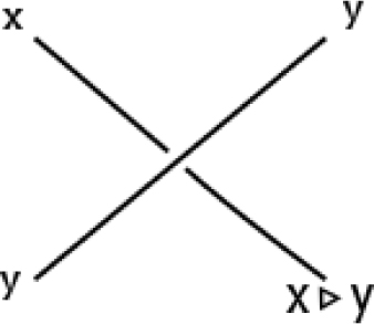
The coloring of a regular crossing with one operation
Definition 2.1
A kei (involutory quandle) is a setXwith a binary operation ▹ : X × X → Xsatifying the following three axioms:
x ▹ x = x, for allx ∈ X.
(x ▹ y)▹ y = x, for allx, y ∈ X.
(x ▹ y)▹ z = (x ▹ z) ▹ (y ▹ z), for allx, y, z ∈ X.
The three axioms of a kei result from the invariance of the three Reidemeister moves as in the following figures.

The coloring of Reidemeister moves
Now, instead of one operation at a crossing, two operations are defined, and instead of coloring the arcs from the top, the arcs are colored from left to right, so we get:
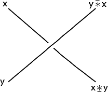
The coloring of a regular crossing with two operations
Next we give the definition of a bikei. After this we will see how the axioms of a bikei result from the three Reidemeister moves.
Definition 2.2
A bikei (involutory biquandle) is a setXwith two binary operations*, * : X × X → Xsuch that for allx, y, z ∈ X, we have
The axioms of a bikei result from the invariance of the three Reidemeister moves as in figures 4, 6 and 7.

Reidemeister move RI for bikei
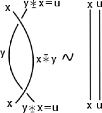
Reidemeister move RII for bikei
Rotated coloring crossing

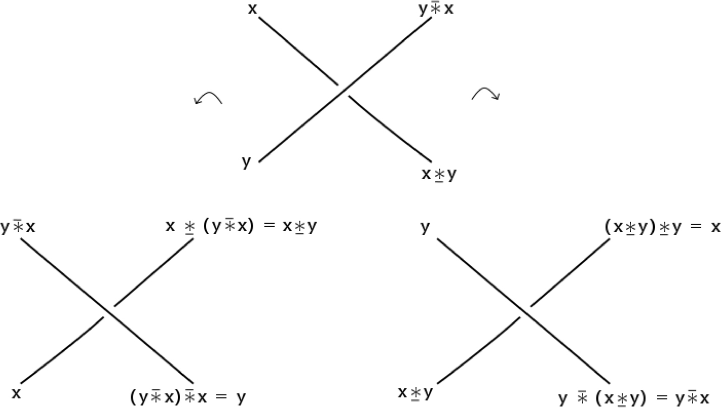
Reidemeister move RIII for bikei
The Reidemeister move RIII gives us what is called the exchange laws:
The Reidemeister move RII means that the over crossing and under crossing operations do not depend on which way the crossing is rotated.
Let X and Y be bikei with operations *X, *X and *Y, *Y respectively. Then a map f : X ⟶ Y is a bikei homomorphism if for all x, x′ ∈ X we have
A bikei isomorphism is a bijective bikei homomorphism, and two bikei are isomorphic if there is a bikei isomorphism between them.
Remark 2.3
Every Kei is a bikei with the operationsx*y = x ▹ yandx*y = x.
Typical examples of bikei include the following :
A non-empty set X with operation x*y = x*y = σ(x), where σ is any involution from X to X, is a bikei. It is called a constant action bikei.
Let Λ = Z[t, s]/(t2 − 1, s2 − 1, (s − t)(1 − s)), then any Λ - module X with x*y = tx + (s − t)y, and x*y = sx, is called an Alexander bikei.
A group X = G with x*y = yx−1y and x*y = x is a bikei. It is called the core bikei of the group G.
A singular link in S3 is the image of a smooth immersion of n circles in S3 that has finitely many double points, called singular points.
Two singular knots K1 and K2 are isotopy equivalent if we can get one of them from the other by a finite sequence of the generalized Reidemeister moves RI, RII, RIII, RIVa, RIVb and RV in the following figure.

Generalized Reidemeister moves RI, RII, RIII, RIVa, RIVb and RV
3 Construction of singbikei
We will define the notion of a singbikei and give some examples and use them to construct an invariant of singular knots and links. The invariant is the set of colorings of a given singular knot or link by a singbikei. We draw the colorings of the regular and singular crossings as in the following figure.
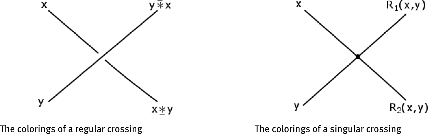
Since our singular crossings are unoriented, we need the operations to be symmetric in the sense that if we rotate the crossing in the right diagram of the above figure by 90, 180 or 270 degrees, the operations should stay the same in order for colorings to be well-defined. Therefore we get the following three axioms:
We have 5 generalized Reidemeister moves; I, II, III are for regular crossings; IV, V are for singular crossings. Next we show how the generalized Reidemeister moves induce relations considering the colorings of the singular crossings.
The following definition is coming from the generalized Reidemeister moves and the axioms are justified from the figures [9-11].

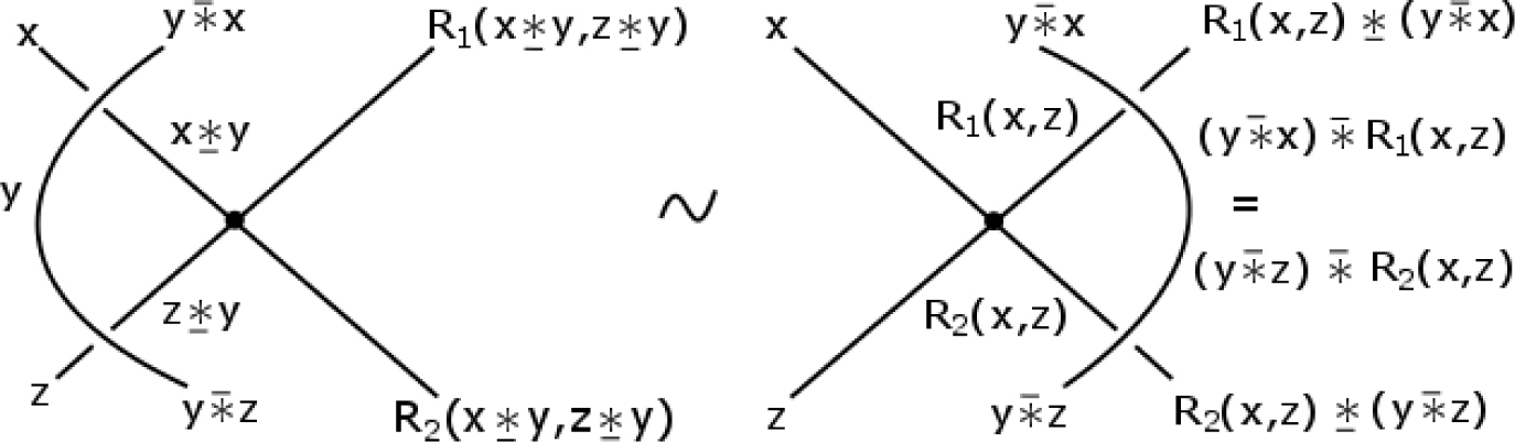
Reidemeister move RIVa
Reidemeister move RIVb
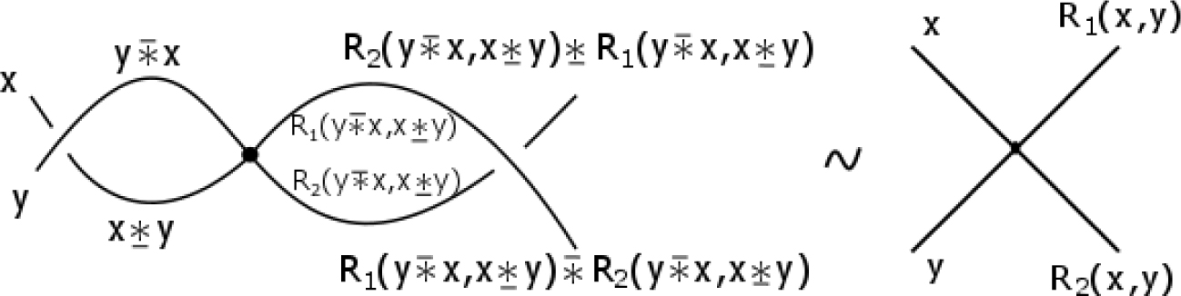
Reidemeister move RV
Definition 3.1
Let (X, *, *) be a bikei. LetR1andR2be two maps fromX × Xto X. Then (X, *, *, R1, R2) is called a singbikei if, in addition to the three axioms 3.1, 3.2 and 3.3, the following axioms are satisfied
The following straightforward lemma makes the set of colorings of a singular knot or link by a singbikei an invariant of singular knots and links.
Lemma 3.2
The set of colorings of a singular knot by a singbikei does not change by the Reidemeister moves RI, RII, RIII, RIVa, RIVb and RV.
Example 3.3
It is known that every kei is a bikei with the operationsx*y = x ▹ yandx*y = x. ThenXis a bikei with these operations so (X, *,*,R1, R2) is a singbikei ifR1, R2 : X × X ⟶ Xsatisfy the following equations:
Example 3.4
LetXbe a set andσ : X ⟶ Xbe any involution onX, (i.e any map such thatσ2 = IdX) withx*y = x*y = σ(x).
LetR1, R2 : X × X ⟶ Xbe two maps, then (X, *, *, R1, R2) is a singbikei ifR1andR2satisfy the following equations:
Proposition 3.5
Let X = Znandσ : Zn ⟶ Znbe given by one of the following rules
or
or
thenσis an involution.
Proof
If σ is given by σ (x)= (n − 1)x + d, then
If σ is given by σ (x)= x, then
If σ is given by
This completes the proof. □
Sometimes these are the only linear (i.e functions of the form f(x)= ax + b) involutions σ on Zn and sometimes Zn has other linear involutions. For example if X = Z8, in addition to the previous solutions,
are also linear involutions in Z8.
Lemma 3.6
Ifnis prime, then the only linear formulas for an involutionσonZnare:
Proof
The general linear formula of σ is σ (x)= cx + d, where c, d ∈ Zn.
Since σ is an involution, we have
Since c2 = 1 in Zn and n is prime, we have
So, we have two cases:
If c = n − 1, then
Therefore σ (x)= (n − 1)x + d, where d ∈ Zn.
If c = 1, then
If d = 0, then σ (x)= x.
If
So σ must be σ (x)= (n − 1)x + d, d ∈ Zn or σ (x) = x.
Theorem 3.7
LetX = Znandσ : Zn ⟶ Znbe an involution andx*y = x*y = σ(x). ThenR1, R2 : Zn × Zn ⟶ Zngiven below make (Zn, *, *, R1, R2) a singbikei.
Ifσ (x) = (n − 1)x + d, d ∈ Znthen
R1(x, y) = (n − 1)y + cwhen (n − 2)d = (n − 2)c and
R2(x, y)= (n − 1)x + c.
Ifσ (x) = x, then
R1(x, y)= (n − 1)y + cand
R2(x, y) = (n − 1)x + c.
Ifσ (x) =
R1(x, y) = (n − 1)y + cwhen
R2(x, y) = (n − 1)x + c.
Proof
We show that R1 and R2 satisfy all the equations in Example 3.4,
If σ (x)= (n − 1)x + d, where d ∈ Zn, then
Let I = σ(R2(σ(y), σ(x)).
Let H = σ(R1(σ(y), σ(x)).
If σ(x) = x, then
If σ(x) = x +
So (Zn,*, *, R1, R2) is a singbikei. □
Example 3.8
As examples on the last theorem, we give
let X = Z10, with
then (Z10,*, *, R1, R2) is a singbikei.
let X = Z8, with
then (Z8, *, *, R1, R2) is a singbikei.
Example 3.9
LetΛ = Z[t, s]/(t2–1 , s2–1, (s–t)(1–s)) be the quotient of the ring of two-variable polynomials with integer coefficients such that s2 = t2 = 1 by the ideal generated by (s–t)(1–s). LetR1, R2 : X × X ⟶ Xbe two maps. Then anyΛ - module X with x*y = tx + (s–t)y, and x*y = sx, is a singbikei ifR1andR2satisfy the following equations:
We call such a singbikei an Alexander singbikeis. For example,
Z10 with x*y = 9x + 2y and x*y = x, R1(x, y) = 8x + 3y and R2(x, y) = 7x + 4y satisfy all the equations in Example 3.9. So (Z10, * ,*, R1,R2) is an Alexander singbikei.
Z13 with x*y = 12x + 2y and x*y = x, R1(x, y) = 9x + 5y and R2(x, y) = 8x + 6y satisfy all the equations in Example 3.9. So (Z13, * ,*, R1,R2) is an Alexander singbikei.
Example 3.10
Let X = G be a group withx*y = yx−1y andx*y = x.
LetR1 , R2 : X × X ⟶ X be two maps, then (X, *, *, R1, R2) is a singbikei ifR1andR2satisfy the following equations:
Proposition 3.11
The following maps
with the condition
are solutions for the system inExample 3.10.
Proof
We show that R1 and R2 satisfy the equations in Example 3.10.
This completes the proof. □
Remark 3.12
From the proposition above, note that:
If n = 1 , thenR1(x, y) = xy–1x andR2(x, y) = x with the condition (yx–1)2 = 1 is a solution forExample 3.10.
If n = 2 , thenR1(x, y) = xy–1xy–1x andR2(x, y) = xy–1x with the condition (yx–1)5 = 1 is a solution forExample 3.10.
4 Applications
In this section we use singbikei and coloring invariants to distinguish singular knots and links.
Example 4.1
Consider the two singular knots in the graph below.
(a) Let X = G be a group generated by (yx–1)2 = 1 with x*y = yx–1y and x*y = x, R1(x, y) = xy–1x andR2 (x, y) = x.
In Figure 12(a), the relations at the crossings give
The singular knots in Example 4.1(a).
Thus the set of colorings is {(x, y, z) ∈ G × G × G : x = y = z}.
In Figure 12(b), the relations at the crossings give
Thus the set of colorings is {(x, y, z) ∈ G × G × G : x = y = z}.
The solution set is the same for both of the sets of colorings above. Therefore, this coloring invariant fails to distinguish these two singular knots.
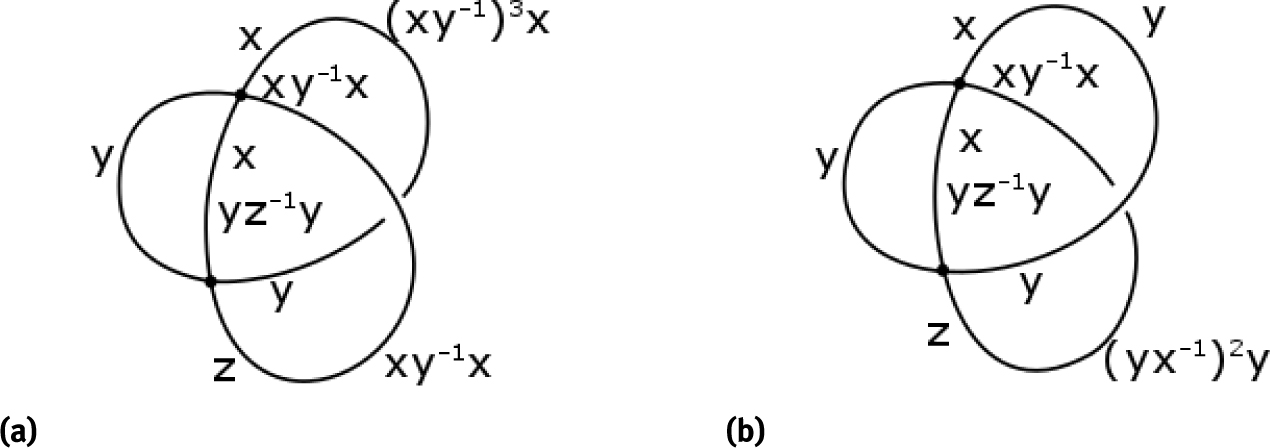
(b) Let X = G be a group generated by (yx–1)5 = 1 with x*y = yx–1y and x*y = x, R1(x, y) = (xy–1)2x and R2 (x, y) = xy–1x.
In Figure 13(a), the relations at the crossings give
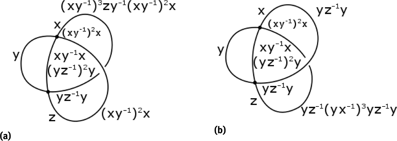
The singular knots in Example 4.1(b).
Thus the set of colorings is {(x, y, z) ∈ G × G × G: 1 = (xy–1)3, (xy–1)2 = (yz–1)2}.
In Figure 13(b), the relations at the crossings give
Thus the set of colorings is {(x, y, z) ∈ G × G × G: xy–1 = yz–1}.
One can always choose a group G such that these two coloring sets are distinct.
Example 4.2
Consider the two singular links in the graph below, let X = G be a group generated by (yx–1)5 = 1 with x*y = yx–1y and x*y = x, R1(x, y) = (xy–1)2x andR2 (x, y) = xy–1x.
In Figure 14(a), the relations at the crossings give

The singular links in Example 4.2.
Thus the set of colorings is {(x, y, z) ∈ G × G × G : x = y = z}.
In Figure 14(b), the relations at the crossings give
Thus the set of colorings is {(x, y, z) ∈ G × G × G : x = y, 1 = (yz–1)3}.
One can always choose a group G such that these two coloring sets are distinct.
Example 4.3
Consider the two singular links in the graph below. Each of them has one singular crossing followed by (n + 1) regular crossings, let X = G be a group generated by (yx–1)5 = 1 with x*y = yx–1y and x*y = x, R1(x, y) = (xy–1)2x andR2 (x, y) = xy–1x.
In Figure 15(a), the relations at the crossings give
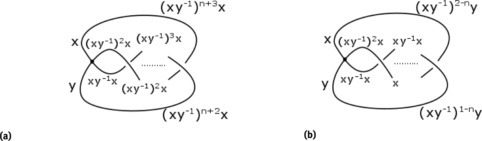
The singular links in Example 4.3.
Thus the set of colorings is {(x, y) ∈ G × G : 1 = (xy–1)n+3}.
In Figure 15(b), the relations at the crossings give
Thus the set of colorings is {(x, y) ∈ G × G : 1 = (xy–1)1–n}.
One can always choose a group G such that these two coloring sets are distinct.
Example 4.4
Consider the two singular knots in the graph below, let X = G be a group generated by (yx–1)5 = 1 with x*y = yx–1y and x*y = x, R1(x, y) = (xy–1)2x andR2 (x, y) = xy–1x.
In Figure 16(a), the relations at the crossings give
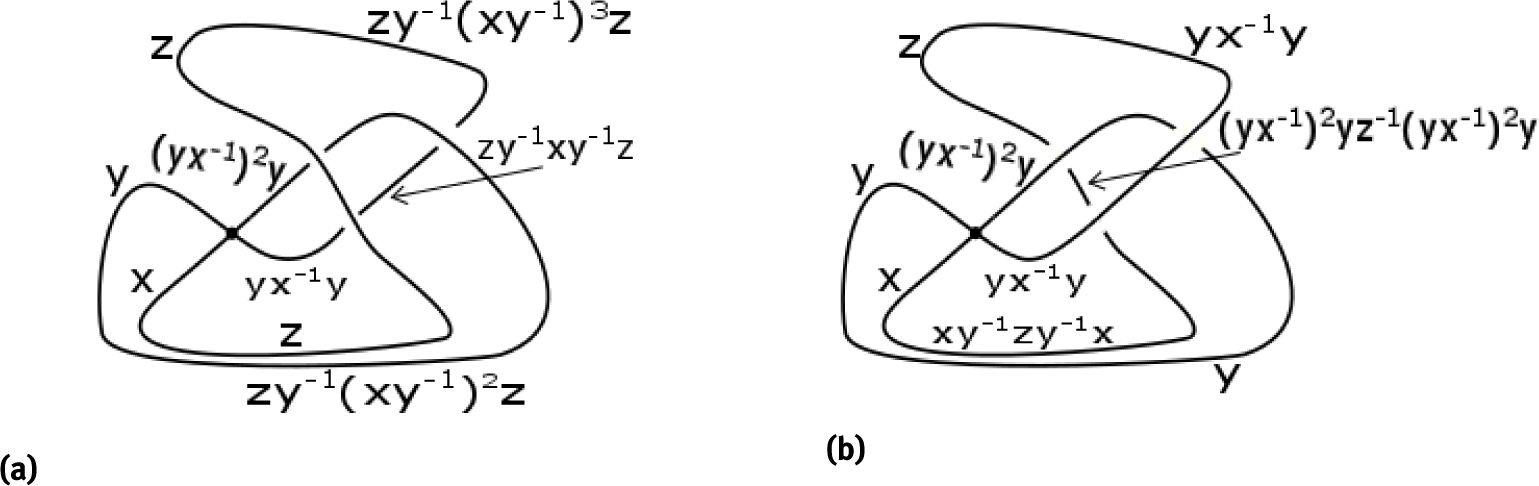
The singular knots in Example 4.4.
Thus the set of colorings is {(x, y, z) ∈ G × G × G : x = z, 1 = (xy–1)4}.
In Figure 16(b), the relations at the crossings give
Thus the set of colorings is {(x, y, z) ∈ G × G × G : z = yx–1y}.
Therefore, this coloring invariant distinguishes these two singular knots.
Example 4.5
Consider the two singular knots in the graph below, let X = G be a group generated by (yx–1)5 = 1 with x*y = yx–1y and x*y = x, R1(x, y) = (xy–1)2x andR2(x, y) = xy–1x.
In Figure 17(a), the relations at the crossings give
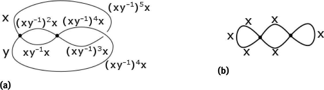
The singular knots in Example 4.5.
Thus the set of colorings is G × G.
In Figure 17(b), the set of colorings is G. Therefore, this coloring invariant distinguishes these two singular knots.
Acknowledgement
The second author would like to thank her masters thesis advisor, the first author, for his guidance and big efforts to accomplish this work.
References
[1] Birman JS., New points of view in knot theory, Bulletin of the American Mathematical Society, 1993, 28, 253-87.10.1090/S0273-0979-1993-00389-6Search in Google Scholar
[2] Birman JS., Lin XS., Knot polynomials and Vassiliev’s invariants, Inventiones mathematicae, 1993, 111, 225-70.10.1007/BF01231287Search in Google Scholar
[3] Vassiliev VA., Cohomology of knot spaces, Theory of singularities and its applications, 1990, 1, 23-69.10.1090/advsov/001/03Search in Google Scholar
[4] Bataineh K., Elhamdadi M., Hajij M., The colored Jones polynomial of singular knots, New York J. Math., 2016, 22, 1439-56.Search in Google Scholar
[5] Fiedler T., The Jones and Alexander polynomials for singular links, Journal of Knot Theory and Its Ramifications, 2010, 19, 859-66.10.1142/S0218216510008236Search in Google Scholar
[6] Kauffman LH., Invariants of graphs in three-space, Transactions of the American Mathematical Society, 1989, 311, 697-710.10.1090/S0002-9947-1989-0946218-0Search in Google Scholar
[7] Juyumaya J., Lambropoulou S., An invariant for singular knots, Journal of Knot Theory and Its Ramifications, 2009, 18, 825-40.10.1142/S0218216509007324Search in Google Scholar
[8] Kauffman LH., Vogel P., Link polynomials and a graphical calculus, Journal of Knot Theory and Its Ramifications, 1992, 1, 59-104.10.1142/S0218216592000069Search in Google Scholar
[9] Carter JS., Silver DS., Williams SG., Elhamdadi M., Saito M., Virtual knot invariants from group biquandles and their cocycles, Journal of Knot Theory and Its Ramifications, 2009, 18, 957-72.10.1142/S0218216509007269Search in Google Scholar
[10] Clark WE., Elhamdadi M., Saito M., Yeatman T., Quandle colorings of knots and applications, Journal of knot theory and its ramifications, 2014, 23, 1450035.10.1142/S0218216514500357Search in Google Scholar PubMed PubMed Central
[11] Elhamdadi M., Nelson S., Quandles, American Mathematical Soc., 2015, 47.10.1090/stml/074Search in Google Scholar
[12] Henrich A., Nelson S., Semiquandles and flat virtual knots, Pacific journal of mathematics, 2010, 248, 155-70.10.2140/pjm.2010.248.155Search in Google Scholar
[13] Chien J., Nelson S., Virtual Links with Finite Medial Bikei, arXiv preprint arXiv:1704.00812, 2017.10.1016/j.jsc.2018.04.015Search in Google Scholar
[14] Nelson S., Rivera P., Bikei invariants and gauss diagrams for virtual knotted surfaces, Journal of Knot Theory and Its Ramifications, 2016, 25, 1640008.10.1142/S0218216516400083Search in Google Scholar
[15] Joyce D., A classifying invariant of knots, the knot quandle, Journal of Pure and Applied Algebra, 1982, 23, 37-65.10.1016/0022-4049(82)90077-9Search in Google Scholar
[16] Przytycki J., 3-coloring and other elementary invariants of knots, Banach Center Publications, 1998, 42, 275-95.10.4064/-42-1-275-295Search in Google Scholar
[17] Wada M., Group invariants of links, Topology, 1992, 31, 399-406.10.1016/0040-9383(92)90029-HSearch in Google Scholar
[18] Churchill IR., Elhamdadi M., Hajij M., Nelson S., Singular knots and involutive quandles, Journal of Knot Theory and Its Ramifications, 2017, 26, 1750099.10.1142/S0218216517500997Search in Google Scholar
[19] Bataineh K., Elhamdadi M., Hajij M., Youmans W., Generating sets of Reidemeister moves of oriented singular links and quandles, arXiv preprint arXiv:1702.01150, 2017.10.1142/S0218216518500645Search in Google Scholar
© 2018 Bataineh and Ghaith, published by De Gruyter
This work is licensed under the Creative Commons Attribution-NonCommercial-NoDerivatives 4.0 License.
Articles in the same Issue
- Regular Articles
- Algebraic proofs for shallow water bi–Hamiltonian systems for three cocycle of the semi-direct product of Kac–Moody and Virasoro Lie algebras
- On a viscous two-fluid channel flow including evaporation
- Generation of pseudo-random numbers with the use of inverse chaotic transformation
- Singular Cauchy problem for the general Euler-Poisson-Darboux equation
- Ternary and n-ary f-distributive structures
- On the fine Simpson moduli spaces of 1-dimensional sheaves supported on plane quartics
- Evaluation of integrals with hypergeometric and logarithmic functions
- Bounded solutions of self-adjoint second order linear difference equations with periodic coeffients
- Oscillation of first order linear differential equations with several non-monotone delays
- Existence and regularity of mild solutions in some interpolation spaces for functional partial differential equations with nonlocal initial conditions
- The log-concavity of the q-derangement numbers of type B
- Generalized state maps and states on pseudo equality algebras
- Monotone subsequence via ultrapower
- Note on group irregularity strength of disconnected graphs
- On the security of the Courtois-Finiasz-Sendrier signature
- A further study on ordered regular equivalence relations in ordered semihypergroups
- On the structure vector field of a real hypersurface in complex quadric
- Rank relations between a {0, 1}-matrix and its complement
- Lie n superderivations and generalized Lie n superderivations of superalgebras
- Time parallelization scheme with an adaptive time step size for solving stiff initial value problems
- Stability problems and numerical integration on the Lie group SO(3) × R3 × R3
- On some fixed point results for (s, p, α)-contractive mappings in b-metric-like spaces and applications to integral equations
- On algebraic characterization of SSC of the Jahangir’s graph 𝓙n,m
- A greedy algorithm for interval greedoids
- On nonlinear evolution equation of second order in Banach spaces
- A primal-dual approach of weak vector equilibrium problems
- On new strong versions of Browder type theorems
- A Geršgorin-type eigenvalue localization set with n parameters for stochastic matrices
- Restriction conditions on PL(7, 2) codes (3 ≤ |𝓖i| ≤ 7)
- Singular integrals with variable kernel and fractional differentiation in homogeneous Morrey-Herz-type Hardy spaces with variable exponents
- Introduction to disoriented knot theory
- Restricted triangulation on circulant graphs
- Boundedness control sets for linear systems on Lie groups
- Chen’s inequalities for submanifolds in (κ, μ)-contact space form with a semi-symmetric metric connection
- Disjointed sum of products by a novel technique of orthogonalizing ORing
- A parametric linearizing approach for quadratically inequality constrained quadratic programs
- Generalizations of Steffensen’s inequality via the extension of Montgomery identity
- Vector fields satisfying the barycenter property
- On the freeness of hypersurface arrangements consisting of hyperplanes and spheres
- Biderivations of the higher rank Witt algebra without anti-symmetric condition
- Some remarks on spectra of nuclear operators
- Recursive interpolating sequences
- Involutory biquandles and singular knots and links
- Constacyclic codes over 𝔽pm[u1, u2,⋯,uk]/〈 ui2 = ui, uiuj = ujui〉
- Topological entropy for positively weak measure expansive shadowable maps
- Oscillation and non-oscillation of half-linear differential equations with coeffcients determined by functions having mean values
- On 𝓠-regular semigroups
- One kind power mean of the hybrid Gauss sums
- A reduced space branch and bound algorithm for a class of sum of ratios problems
- Some recurrence formulas for the Hermite polynomials and their squares
- A relaxed block splitting preconditioner for complex symmetric indefinite linear systems
- On f - prime radical in ordered semigroups
- Positive solutions of semipositone singular fractional differential systems with a parameter and integral boundary conditions
- Disjoint hypercyclicity equals disjoint supercyclicity for families of Taylor-type operators
- A stochastic differential game of low carbon technology sharing in collaborative innovation system of superior enterprises and inferior enterprises under uncertain environment
- Dynamic behavior analysis of a prey-predator model with ratio-dependent Monod-Haldane functional response
- The points and diameters of quantales
- Directed colimits of some flatness properties and purity of epimorphisms in S-posets
- Super (a, d)-H-antimagic labeling of subdivided graphs
- On the power sum problem of Lucas polynomials and its divisible property
- Existence of solutions for a shear thickening fluid-particle system with non-Newtonian potential
- On generalized P-reducible Finsler manifolds
- On Banach and Kuratowski Theorem, K-Lusin sets and strong sequences
- On the boundedness of square function generated by the Bessel differential operator in weighted Lebesque Lp,α spaces
- On the different kinds of separability of the space of Borel functions
- Curves in the Lorentz-Minkowski plane: elasticae, catenaries and grim-reapers
- Functional analysis method for the M/G/1 queueing model with single working vacation
- Existence of asymptotically periodic solutions for semilinear evolution equations with nonlocal initial conditions
- The existence of solutions to certain type of nonlinear difference-differential equations
- Domination in 4-regular Knödel graphs
- Stepanov-like pseudo almost periodic functions on time scales and applications to dynamic equations with delay
- Algebras of right ample semigroups
- Random attractors for stochastic retarded reaction-diffusion equations with multiplicative white noise on unbounded domains
- Nontrivial periodic solutions to delay difference equations via Morse theory
- A note on the three-way generalization of the Jordan canonical form
- On some varieties of ai-semirings satisfying xp+1 ≈ x
- Abstract-valued Orlicz spaces of range-varying type
- On the recursive properties of one kind hybrid power mean involving two-term exponential sums and Gauss sums
- Arithmetic of generalized Dedekind sums and their modularity
- Multipreconditioned GMRES for simulating stochastic automata networks
- Regularization and error estimates for an inverse heat problem under the conformable derivative
- Transitivity of the εm-relation on (m-idempotent) hyperrings
- Learning Bayesian networks based on bi-velocity discrete particle swarm optimization with mutation operator
- Simultaneous prediction in the generalized linear model
- Two asymptotic expansions for gamma function developed by Windschitl’s formula
- State maps on semihoops
- 𝓜𝓝-convergence and lim-inf𝓜-convergence in partially ordered sets
- Stability and convergence of a local discontinuous Galerkin finite element method for the general Lax equation
- New topology in residuated lattices
- Optimality and duality in set-valued optimization utilizing limit sets
- An improved Schwarz Lemma at the boundary
- Initial layer problem of the Boussinesq system for Rayleigh-Bénard convection with infinite Prandtl number limit
- Toeplitz matrices whose elements are coefficients of Bazilevič functions
- Epi-mild normality
- Nonlinear elastic beam problems with the parameter near resonance
- Orlicz difference bodies
- The Picard group of Brauer-Severi varieties
- Galoisian and qualitative approaches to linear Polyanin-Zaitsev vector fields
- Weak group inverse
- Infinite growth of solutions of second order complex differential equation
- Semi-Hurewicz-Type properties in ditopological texture spaces
- Chaos and bifurcation in the controlled chaotic system
- Translatability and translatable semigroups
- Sharp bounds for partition dimension of generalized Möbius ladders
- Uniqueness theorems for L-functions in the extended Selberg class
- An effective algorithm for globally solving quadratic programs using parametric linearization technique
- Bounds of Strong EMT Strength for certain Subdivision of Star and Bistar
- On categorical aspects of S -quantales
- On the algebraicity of coefficients of half-integral weight mock modular forms
- Dunkl analogue of Szász-mirakjan operators of blending type
- Majorization, “useful” Csiszár divergence and “useful” Zipf-Mandelbrot law
- Global stability of a distributed delayed viral model with general incidence rate
- Analyzing a generalized pest-natural enemy model with nonlinear impulsive control
- Boundary value problems of a discrete generalized beam equation via variational methods
- Common fixed point theorem of six self-mappings in Menger spaces using (CLRST) property
- Periodic and subharmonic solutions for a 2nth-order p-Laplacian difference equation containing both advances and retardations
- Spectrum of free-form Sudoku graphs
- Regularity of fuzzy convergence spaces
- The well-posedness of solution to a compressible non-Newtonian fluid with self-gravitational potential
- On further refinements for Young inequalities
- Pretty good state transfer on 1-sum of star graphs
- On a conjecture about generalized Q-recurrence
- Univariate approximating schemes and their non-tensor product generalization
- Multi-term fractional differential equations with nonlocal boundary conditions
- Homoclinic and heteroclinic solutions to a hepatitis C evolution model
- Regularity of one-sided multilinear fractional maximal functions
- Galois connections between sets of paths and closure operators in simple graphs
- KGSA: A Gravitational Search Algorithm for Multimodal Optimization based on K-Means Niching Technique and a Novel Elitism Strategy
- θ-type Calderón-Zygmund Operators and Commutators in Variable Exponents Herz space
- An integral that counts the zeros of a function
- On rough sets induced by fuzzy relations approach in semigroups
- Computational uncertainty quantification for random non-autonomous second order linear differential equations via adapted gPC: a comparative case study with random Fröbenius method and Monte Carlo simulation
- The fourth order strongly noncanonical operators
- Topical Issue on Cyber-security Mathematics
- Review of Cryptographic Schemes applied to Remote Electronic Voting systems: remaining challenges and the upcoming post-quantum paradigm
- Linearity in decimation-based generators: an improved cryptanalysis on the shrinking generator
- On dynamic network security: A random decentering algorithm on graphs