
Disjointed sum of products by a novel technique of orthogonalizing ORing
-
Yavuz Can


Abstract
This work presents a novel combining method called ‘orthogonalizing ORing
1 Introduction
A Boolean function or a switching function, respectively, is defined as a mapping f(x) : Bn → B with B = {0, 1}. It can be expressed by using Boolean variables xi = {x1, x2, …, xn} [1, 3, 10, 14, 20, 21]. As shown in Table 1, Boolean variables which are either direct xn or negated x̄n are connected by operations like conjunction (∧, or no operation sign), disjunction (∨), antivalence (⊕) and equivalence (⊙).
Boolean operations of two variables
| xi | xj | x̄i | x̄j | xi ∧ xj | xi ∨ xj | xi ⊕ xj | xi ⊙ xj |
|---|---|---|---|---|---|---|---|
| 0 | 0 | 1 | 1 | 0 | 0 | 0 | 1 |
| 0 | 1 | 1 | 0 | 0 | 1 | 1 | 0 |
| 1 | 0 | 0 | 1 | 0 | 1 | 1 | 0 |
| 1 | 1 | 0 | 0 | 1 | 1 | 0 | 1 |
There are four standard forms fS(x) of switching function [1, 6, 19] which are either connected by conjunctions
Definition 1.1
(Standard Forms with m ∈ ℕ ∖ {1}).
2 Characteristic of orthogonality
The characteristic of orthogonality is a special attribute of a switching function [1, 5, 6, 15, 16, 17, 18]. The orthogonal form of a switching function is characterized by conjunctions or disjunctions which are disjointed to one another in pairs. This means, that for each pair of conjunctions, one of them contains a direct Boolean variable (xi) and the other contains the negation (x̄i) of the same Boolean variable. Consequently, the intersection of each pair of these conjunctions (ci,j(x)) results in 0, as shown in Eq. (5). In contrast, the disjunction of each pair of orthogonal disjunctions (di,j(x)) results in 1, as shown in Eq. (6).
Definition 2.1
(Orthogonality of Conjunctions or Disjunctions). Two conjunctionsci(x) andcj(x) are orthogonal to each other if the following applies:
Two disjunctionsdi(x) anddj(x) are orthogonal to each other if the following applies:
The orthogonal form of a fS(x) enables its transformation in another form, which will have equivalent function values. This means, that the native form and the transformed form have the same function values if the same input values are used in each case. Therefore, orthogonalization simplifies the handling for further calculation steps, especially in the application of electrical engineering, e.g. for further calculation step as the Boolean Differential Calculus (BDC) [2, 3] by which all possible test patterns for a combinational circuit can be determined. Test patterns are used to detect feasible faults in combinational circuits. Additionally, it facilitates the calculation of BDC particularly in Ternary-Vector-List (TVL) arithmetic [11, 12, 16, 17, 18]. TVL is a kind of matrix which simplifies the computational representation of Boolean functions and their computational handling of tasks in a facilitated way.
Theorem 2.2
(Orthogonality of DF and AF). If the intersection of every two conjunctionsci,j(x) of a given DF is 0 thenDForth = AForthapplies. That means, an orthogonal disjunctive formDForthis equivalent to the orthogonal antivalence formAForthincluding the same conjunctions[1, 3, 10, 14, 15, 21]:
Proof of Theorem 2.2
By using (5) for orthogonal conjunctions ci,j(x) the relation in (7) applies. The respective proof is brought by the following relation. The disjunction of two conjunctions ci,j(x) on the right side is equivalent to the antivalence operation of the same two conjunctions on the right side. This is the procedure of reshaping of a disjunctive form in the antivalence form. For the case that both conjunctions are orthogonal the last term on the right side results in 0. An antivalence-operation with 0 is to be neglected, as xi ⊕ 0 = xi applies. Consequently, this leads to the relation in (7).
□
Theorem 2.3
(Orthogonality of CF and EF). If the union of every two disjunctionsdi,j(x) of a given CF is 1 thenCForth = EForthapplies. Thus, an orthogonal conjunctive formCForthis equivalent to the orthogonal equivalence formEForthincluding the same disjunctions[1, 3, 10, 14, 15, 21]:
Proof of Theorem 2.3
A CF can be represented as an EF by using the following condition in (10). By using (6) for orthogonal disjunctions di,j(x) in this case the relation in (9) applies. The conjunction of two disjunctions di,j(x), that means a CF, on the left side is equivalent to the right side which illustrates the equivalence operation of the same two disjunctions. If these both disjunctions di,j(x) are orthogonal then the union of them results in 1, as shown by the last term on the right side. An equivalence-operation with 1 is to be neglected, as xi ⊙ 1 = xi applies. Consequently, the relation in (9) applies.
□
3 Elementary operations of two conjunctions
In this section the elementary operations (intersection, union, difference-building) of conjunctions, which are deduced out of the set theory due to the isomorphism, are defined for the switching algebra. These formulas for different operations of conjunctions specify the order in which the variables of the given conjunction have to be linked. That means, if a variable is displayed negated, the corresponding literal of the given conjunction must be negated at this point. The number of variables in their respective conjunction is defined by n or n′.
Theorem 3.1
(Intersection of two conjunctions). The intersection of any two conjunctionsci,j(x) withn, n′ ∈ ℕ is calculated by:
Theorem 3.2
(Union of two conjunctions). The union of any two conjunctionsci,j(x) withn, n′ ∈ ℕ is given by:
Theorem 3.3
(Difference-building of two conjunctions). The difference-building of a conjunctioncm(x) as minuend and another conjunctioncs(x) as subtrahend withn, n′ ∈ ℕ is calculated by following equation, which is deduced out of the set theory[4, 13]. That means, for the difference of two setsM − Sit appliesM ∩ S̄which is transferred to the switching algebra due to the isomorphism. Consequently, the difference-building of two conjunctions is the intersection of the minuend and the complement of the subtrahend. By building the difference several conjunctions arise which are not disjointed (orthogonal) to each other.
4 Orthogonalizing difference-building
The technique of orthogonalizing difference-building ⊖ is used to calculate the orthogonal difference of two conjunctions (ci,j(x)) whereby the result is orthogonal. This method is generally valid and equivalent to the usual method of difference-building [6, 7, 8, 9]. Orthogonalizing difference-building ⊖ is the composition of two calculation steps - the difference-building and the subsequent orthogonalization.
Definition 4.1
(Orthogonalizing difference-building). Orthogonalizing difference-building ⊖ corresponds to the removal of the intersection which is formed between the minuend conjunctioncm(x) and the subtrahend conjunctioncs(x) from the minuendcm(x), which meanscm(x) - (cm(x) ∧ cs(x)); the result is orthogonal. Orthogonalizing difference-building of two conjunctions withn, n′ ∈ ℕ is defined as:
In this case, the formula
This method is explained by the following example and description. Additionally, this example is also illustrated in a K-map (Figure 1).
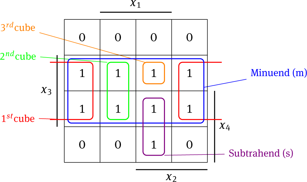
Example 4.2 in a K-map
Example 4.2
A subtrahend (cs(x) = x1x2x4) is subtracted from a minuend (cm(x) = x3). It is a result of several conjunctions (1stcube, 2ndcube, 3rdcube) which are orthogonal to each other and cover all of the remaining 1s.
first literal of the subtrahend, here x1, is complemented and builds the intersection with the minuend, here x3. Consequently, the first conjunction of the difference is x̄1x3.
Then the second literal, here x2, is complemented and forms the intersection with the minuend, and the first literal x1 of the subtrahend is built. Therefore, the second conjunction is x1x̄2x3.
The next literal, here x4, is complemented and forms the intersection with the minuend, and the first literal x1 and second literal x2 of the subtrahend is built. Thus, the third term of the difference is x1x2x3x̄4.
This process is continued until all literals of the subtrahend are singly complemented and linked by building the intersection with the minuend in a separate conjunction.
5 Orthogonalizing ORing
By a further novel technique ‘orthogonalizing ORing
Definition 5.1
(Orthogonalizing ORing). The intersection of a conjunctioncs1(x), called as the first summand, and a second conjunctioncs2(x), called as the second summand, is removed by the method ⊖ from the first summandcs1(x), and the second summandcs2(x) is linked to that subtraction by a disjunction; the result is orthogonal. This procedure is labeled as orthogonalizing ORing and is defined withn, n′ ∈ ℕ as:
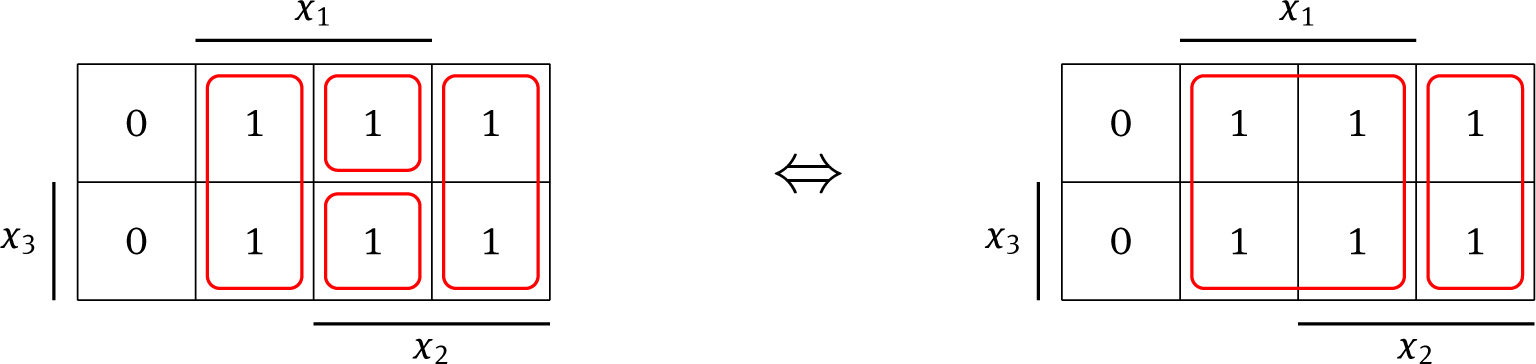
This method of orthogonalizing ORing is explained by the Example 5.2 which is also illustrated in a K-map (Fig. 2).
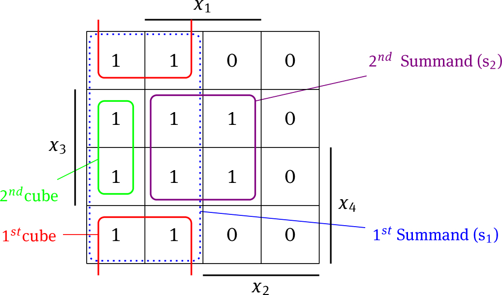
Example 5.2 in a K-map
Example 5.2
The orthogonalizing ORing is built of two conjunctionscs1(x) = x̄2andcs2(x) = x1x3by using Eq. (15).
It is a result of several conjunctions or cubes which are disjointed to each other in pair (Fig. 2). The following points explain this unprecedented technique:
The first literal of the second summand cs2(x), here x1, is complemented and ANDed to the first summand cs1(x). Consequently, the first conjunction of the orthogonal result arises, x̄1x̄2.
Then the second literal of the second summand cs2(x) is complemented, here x3, and ANDed with the first literal of the second summand cs2(x) to the first summand cs1(x). Therefore, the second conjunction of the orthogonal result is developed, x1x̄2x̄3.
This process is continued until all literals of the second summand cs2(x) are singly complemented and linked by ANDing to the first summand cs1(x) in a separate term.
At last the second summand cs2(x) is added to the heretofore calculated conjunctions.
By swapping the position of the summands, the result changes as shown in the following:
However, both solutions are equivalent because the same 1s are covered. They only differ in the form of their coverage. But in order to represent an orthogonal result with a fewer number of conjunctions, the conjunction with more literals has to be accepted as the first summand. That is possible because orthogonalizing ORing has the property of commutativity. By the mathematical induction the general validity of Eq. (15) is given in Proof 1.
The number of conjunctions in the result, called nx, corresponds to the number of literals presented in the second summand cs2(x) and not presented in the first summand cs1(x) at the same time; in addition, a 1 is added to nx, which stands for the second summand cs2(x) as the last linked term. It applies:
Furthermore, the number of possible results, which primarily depends on nx, can be charged by:
Depending on the starting literal the result may differ. There are many equivalent options which only differ in the form of their coverage. This novel technique contains the composition of two calculation procedures – the union ‘∨’ and the subsequent orthogonalization. The result out of orthogonalizing ORing is orthogonal in contrast to the result out of the usual method of union ∨. Both results are different in their representations but cover the same 1s. Hereinafter, the proof of this equivalence between orthogonalizing ORing and union is exemplified. On the left side it is denoted the orthogonalizing ORing of two sets S1, S2 and on the right side the union of the same sets. Due to the axiom of absorption, the equivalence between orthogonalizing ORing and ORing is verified. The right side is the orthogonal form of the left side, which are equivalent but different in their form of coverage.
Proof. 1
General validity of Eq. (15):
∀ (n, n′) ∈ ℕ ∖ {1}, (n, n′) ≥ n0 applies A(n, n′):
if A(n0) ∧ (∀ (n, n′) ∈ ℕ, (n, n′) ≥ n0: A(n, n′) → A((n, n′)+1)) ⇒ ∀ (n, n′) ∈ ℕ, (n, n′) ≥ n0: A(n, n′)
Basis A(n0): n0,
Inductive step A(n, n′) → A(n + 1, n′ + 1): n→ n + 1 and n′ → n′ + 1
□
5.1 Orthogonalizing ORing between a DF and a conjunction
The orthogonalizing ORing of an orthogonal DF f(x)orth and a conjunction cs2(x) can be reached by Eq. (19). With ls1 ∈ ℕ+ as the number of conjunctions in the given function the following applies:
Since the general validity for orthogonalizing ORing is given, there is no need to prove the general validity for Eq. (19) in this case. As shown in Example 5.3 the use of (19) is illustrated.
Example 5.3
Let DFf1(x) = x1 ∨ x2x3and a conjunctionc1(x) = x̄2x̄3. The orthogonalizing ORing between both has to be calculated.
In this case the orthogonal form off1(x) has to be calculated by Eq. (15)otherwise by Eq. (36):
The orthogonal form is generated:
Next step is the application of Eq. (19). Each conjunction off1(x)orthis combined by orthogonalizing ORing withc1(x). However, the adding of the second summand at last is fulfilled after each combining step.
In the K-map on the left side the cubes of f1(x) and c1(x) are represented, and on the K-map on the right side the result after the procedure of orthogonalizing ORing is illustrated (Fig. 3).
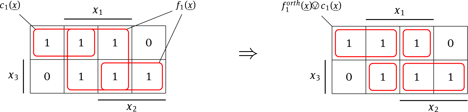
Before and after the process of orthogonalizing ORing
5.2 Axioms and Postulates
5.2.1 Postulates
The following postulates are necessary for getting correct results after each operation of orthogonalizing ORing.
If two conjunctions are already orthogonal to each other (cs1(x) ⊥ cs2(x)) the result corresponds to the disjunction of both conjunctions:
If the first conjunction is the subset of the second conjunction (cs1(x) ⊂ cs2(x)) it follows:
and in the reverse case (cs2(x) ⊂ cs1(x)) it follows:
5.2.2 Axioms for variables
The following rules apply for the linking of variables and constants.
5.2.3 Axioms for conjunctions
Following axioms for conjunctions are deduced out of the axioms for variables.
The neutral element of orthogonalizing ORing is 0:
The result of orthogonalizing ORing between 0 and a conjunction ci(x) is this conjunction ci(x) itself:
The orthogonalizing ORing of a conjunction ci(x) with the unit-term 1 leads to 1:
The result of orthogonalizing ORing between 1 and a conjunction ci(x) is 1:
The result of the orthogonalizing ORing between two the same conjunctions ci(x) results to this conjunction itself:
The orthogonalizing ORing of a conjunction ci(x) with its complement ci(x) results in an unit-term 1:
5.2.4 Commutativity
Commutativity is the property of operation which allows the changing of the terms in their position in such that the value of the expression will not change. As the novel method of orthogonalizing ORing is commutative, the sequence of its execution can be changed.
The value of both sides are equivalent and orthogonal. They can only differ in the form of coverage. The following Example 5.4 gives an overview about the commutative property.
Example 5.4
The left side differs only in the form of coverage in contrast to the right side, which is shown in the corresponding K-maps (Fig. 4). Both sides consist of disjointed cubes.
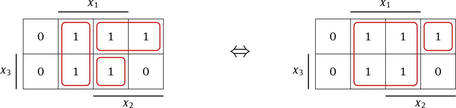
Left and right side of Ex. 5.4
5.2.5 Associativity
Associativity is the property of an operation which allows the rearranging of the parentheses in such that the value of the expression will not change. As orthogonalizing ORing is associative, the position of the parentheses can be changed.
The value of both sides are equivalent and orthogonal. Only the form of their coverage can be different. Following Example 5.5 illustrates this characteristic of associativity.
Example 5.5
Both sides are homogeneous and orthogonal as shown in the K-maps in Figure 5. They only differ in their form of coverage.
Left and right side of Ex. 5.5
5.2.6 Distributivity
The distributive property of an operation allows the exclusion of the same term. That means, that a term can be factored out. Hereby, the orthogonality of both sides has to be insisted. In this case, the distributive law for ANDing out applies for left and right side.
The validity of the distributive property is given by the following proof:
Both sides are equivalent and orthogonal. They can only differ in the form of their coverage. This charasteristic of distributivity is demonstrated by the following Example 5.6 whereby both sides result to the same term.
Example 5.6
6 Disjointed sum of products
Based on this technique of orthogonalizing ORing a novel Equation (36) is formed which enables the orthogonalization of every disjunctive form DF. That means, this formula enables the transformation of a SOP in a homogeneous dSOP. With m ∈ ℕ as the number of conjunctions ci(x) that are included in the given DF, which has to be orthogonalized, it follows that:
The explanation for Equation (36) is provided as follows:
This procedure is continued until the last conjunction cm(x).
The general validity of (36) is proven by the following mathematical induction:
Proof. 2
∀ (m) ∈ ℕ, (m) ≥ m0 applies A(m):
if A(m0) ∧ (∀ (m) ∈ ℕ, m ≥ m0: A(m) → A(m + 1)) ⇒ ∀ (m) ∈ ℕ, m ≥ m0: A(m)
Basis A(m0): m0 = 2
Inductive step A(m) → A(m + 1): m → m + 1
The orthogonal result may differ depending on the order of the conjunctions because of the property of commutativity. Thus, the conjunctions can be changed if necessary. However, all solutions are equivalent and orthogonal. In Example 6.1 it is given an overview of the use of Eq. (36)
Example 6.1
Functionf2(x) = x3 ∨ x1 ∨ x2x̄3has to be orthogonalized by Eq. (36).
Function f2(x)orth is the orthogonal form of function f2(x), illustrated in the K-maps (Fig. 6).
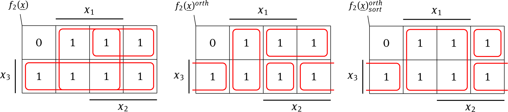
f2(x), f2(x)orth and
By rearrangement of the order of the consisting conjunctions of a DF we obtain fewer number of conjunctions in the derived orthogonal form. This procedure of sorting is carried out from large to small. That means, it takes place from conjunctions of higher number of variables to conjunctions of fewer number of variables. The following Example clarifies this advantage of sorting.
Example 6.2
Functionf2(x) = x3 ∨ x1 ∨ x2x̄3has to be orthogonalized after resorting.
The orthogonalized form of the sorted DF contains fewer number of conjunctions (see Fig. 6).
The analysis of a measurement, as shown in Fig. 7, gives an overview of the comparison of the orthogonalization process depending on sorting. The orthogonalization of unsorted DF called as ORTH[∨] and the sorted of the same DFs called as sortORTH[∨] are compared. Thereby, 50 different functions with five conjunctions were orthogonalized by the novel technique with regards to the tuple length (number of variables) which runs from 1 to 50. Out of these 50 calculations per number of variables the number of conjunctions were determined, from which an average value was calculated for each tuple length. These range of averages were subsequently plotted in the diagram to show the deviation of sortORTH[∨] from ORTH[∨]. This comparison illustrates a reduction of conjunctions in the orthogonal form when the DF was sorted before. This reduction is approximately 19% on average (see Table 2). Additionally, this feature allows the reducing of operation for subsequent calculation steps. Hereby, the relation in (37) is confirmed by the comparison in Fig. 7. The number of conjunctions of an orthogonalized DF
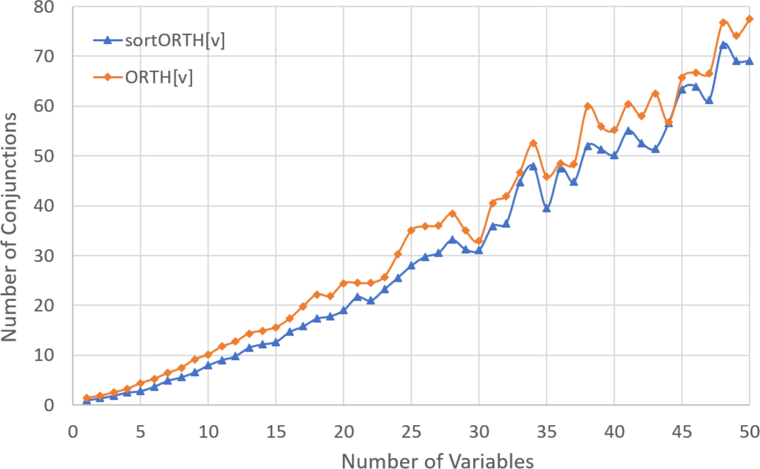
Average number of conjunctions in the orthogonal result
Average number of conjunctions in the orthogonal result
| xn | sortORTH[∨] | ORTH[∨] | deviation in % |
|---|---|---|---|
| 1 | 1 | 1.48 | 48.0 |
| 2 | 1.38 | 1.84 | 33.3 |
| 3 | 1.88 | 2.54 | 35.1 |
| 4 | 2.54 | 3.24 | 27.6 |
| 5 | 2.84 | 4.4 | 54.9 |
| ⋮ | ⋮ | ⋮ | ⋮ |
| 26 | 29.76 | 35.88 | 20.6 |
| 27 | 30.54 | 36.06 | 18.1 |
| 28 | 33.16 | 38.44 | 15.9 |
| 29 | 31.26 | 34.98 | 11.9 |
| ⋮ | ⋮ | ⋮ | ⋮ |
| 46 | 63.96 | 66.72 | 4.3 |
| 47 | 61.26 | 66.52 | 8.6 |
| 48 | 72.28 | 76.84 | 6.3 |
| 49 | 69.02 | 74.06 | 7.3 |
| 50 | 69.02 | 77.46 | 12.2 |
| average deviation in % | 19.3 | ||
7 Conclusion
This work showed a novel technique for building a union of disjointed conjunctions which is called as orthogonalizing ORing. Its results are orthogonal. Orthogonalizing ORing is used to calculate the orthogonal form of building the union of two conjunctions. This linking technique replaces two calculation steps - building a union and the subsequent orthogonalization - by one step. Orthogonalizing ORing is valid in general, which was proven by the mathematical induction, and is also equivalent to the usual method of union ∨. Additionally, postulates related to commutativity, distributivity and associativity and axioms for this method are also defined. Furthermore, every Boolean function of disjunctive form or every Sum of Products, respectively, can easily be orthogonalized mathematically by a novel equation which is based on this linking technique of orthogonalizing ORing. By this orthogonalization a disjointed Sum of Products can be reached in a simpler way. The general validity was also proven by the mathematical induction. An additional step of sorting before the step of orthogonalization achieves a reduction of approximately 19% of the number of conjunctions in the orthogonal result. This feature was illustrated by a measurement whereby the orthogonalization took place before and after sorting.
References
[1] Bochmann, D., Binäre systeme - ein boolean buch, LiLoLe-Verlag, Hagen, Germany, 2006.Search in Google Scholar
[2] Bochmann, D. and Posthoff, Ch., Binäre dynamische systeme, Akademie-Verlag, Berlin, DDR, 1981.Search in Google Scholar
[3] Bochmann, D., Zakrevskij, A. D., and Posthoff, Ch., Boolesche gleichungen. theorie - anwendungen - algorithmen, VEB Verlag Technik, Berlin, DDR, 1984.10.1007/978-3-7091-9507-9Search in Google Scholar
[4] Bronstein, I.N., Musiol, G., Mühlig, H., and Semendjajew, K.A., Taschenbuch der mathematik, Harri Deutsch Verlag, Frankfurt am Main, Thun, Germany, 1999.Search in Google Scholar
[5] Bruni, R., On the Orthogonalization of Arbitrary Boolean Formulae, Journal of Applied Mathematics and Decision Sciences (2005).10.1155/JAMDS.2005.61Search in Google Scholar
[6] Can, Y., Neue Boolesche Operative Orthogonalisierende Methoden und Gleichungen, FAU University Press, Erlangen, Germany, 2016.Search in Google Scholar
[7] Can, Y. and Fischer, G., Orthogonalizing Boolean Subtraction of Minterms or Ternary-Vectors, Acta Physica Polonica A. Special Issue of the International Conference on Computational and Experimental Science and Engineering (ICCESEN 2014) 128 (2015), no. 2B, B–388.Search in Google Scholar
[8] Can, Y. and Fischer, G., Boolean Orthogonalizing Combination Methods, Fifth International Conference on Computational Science, Engineering and Information Technology (CCSEIT 2015) (Vienna, Austria), 23-24 May, 2015.10.5121/csit.2015.51102Search in Google Scholar
[9] Can, Y., Kassim, H., and Fischer, G., New Boolean Equation for Orthogonalizing of Disjunctive Normal Form based on the Method of Orthogonalizing Difference-Building, Journal of Electronic Testing. Theory and Applicaton (JETTA) (April, 2016).10.1007/s10836-016-5572-6Search in Google Scholar
[10] Crama, Y. and Hammer, P. L., Boolean Functions. Theory, Algorithms, and Applications, Cambridge University Press, New York, USA, 2011.10.1017/CBO9780511852008Search in Google Scholar
[11] Kempe, G., Tupel von TVL als Datenstruktur für Boolesche Funktionen, Dissertation, Freiberg, Germany, 2003.Search in Google Scholar
[12] Kühnrich, M., Ternärvektorlisten und deren Anwendung auf binäre Schaltnetzwerke, Dissertation, Karl-Marx-Stadt (Chemnitz), DDR, 1979.Search in Google Scholar
[13] Popula, L., Mathematik für Ingenieure und Naturwissenschaften, Viewer + Teubner Verlag | Springer Fachmedien Wiesbaden GmbH, Wiesbaden, Germany, 2011.10.1007/978-3-8348-8133-5Search in Google Scholar
[14] Posthoff, Ch., Bochmann, D., and Haubold, K., Diskrete Mathematik, BSB Teubner, Leipzig, DDR, 1986.Search in Google Scholar
[15] Posthoff, Ch. and Steinbach, B., Logikentwurf mit XBOOLE. Algorithmen und Programme., Verlag Technik GmbH, Berlin, Germany, 1991.Search in Google Scholar
[16] Steinbach, B. and Dorotska, Ch., Orthogonal Block Building Using Ordered Lists of Ternary Vectors, Freiberg University of Mining and Technology (Freiberg, Germany), 2000.Search in Google Scholar
[17] Steinbach, B. and Dorotska, Ch., Orthogonal Block Change & Block Building Using Ordered Lists of Ternary Vectors, Freiberg University of Mining and Technology (Freiberg, Germany), 2002.Search in Google Scholar
[18] Steinbach, B. and Dorotska, Ch., Orthogonal Block Change & Block Building using a Simulated Annealing Algorithm, Conference on The Experience of Designing and Application of CAD Systems in Microelectronics CADSM 2003, 2003.Search in Google Scholar
[19] Steinbach, B. and Posthoff, Ch., An Extended Theory of Boolean Normal Forms, Proceedings of the 6th Annual Hawaii International Conference on Statistics, Mathematics and Related Fields (Honolulu, Hawaii), p.1124-1139, 2007.Search in Google Scholar
[20] Wuttke, H.-D. and Henke, K., Schaltsysteme. Eine automatenorientierte Einführung, Pearson Deutschland GmbH, München, Germany, 2003.Search in Google Scholar
[21] Zander, H. J., Logischer Entwurf binärer Systeme, Verlag Technik, Berlin, DDR, 1989.Search in Google Scholar
© 2018 Can, published by De Gruyter
This work is licensed under the Creative Commons Attribution-NonCommercial-NoDerivatives 4.0 License.
Articles in the same Issue
- Regular Articles
- Algebraic proofs for shallow water bi–Hamiltonian systems for three cocycle of the semi-direct product of Kac–Moody and Virasoro Lie algebras
- On a viscous two-fluid channel flow including evaporation
- Generation of pseudo-random numbers with the use of inverse chaotic transformation
- Singular Cauchy problem for the general Euler-Poisson-Darboux equation
- Ternary and n-ary f-distributive structures
- On the fine Simpson moduli spaces of 1-dimensional sheaves supported on plane quartics
- Evaluation of integrals with hypergeometric and logarithmic functions
- Bounded solutions of self-adjoint second order linear difference equations with periodic coeffients
- Oscillation of first order linear differential equations with several non-monotone delays
- Existence and regularity of mild solutions in some interpolation spaces for functional partial differential equations with nonlocal initial conditions
- The log-concavity of the q-derangement numbers of type B
- Generalized state maps and states on pseudo equality algebras
- Monotone subsequence via ultrapower
- Note on group irregularity strength of disconnected graphs
- On the security of the Courtois-Finiasz-Sendrier signature
- A further study on ordered regular equivalence relations in ordered semihypergroups
- On the structure vector field of a real hypersurface in complex quadric
- Rank relations between a {0, 1}-matrix and its complement
- Lie n superderivations and generalized Lie n superderivations of superalgebras
- Time parallelization scheme with an adaptive time step size for solving stiff initial value problems
- Stability problems and numerical integration on the Lie group SO(3) × R3 × R3
- On some fixed point results for (s, p, α)-contractive mappings in b-metric-like spaces and applications to integral equations
- On algebraic characterization of SSC of the Jahangir’s graph 𝓙n,m
- A greedy algorithm for interval greedoids
- On nonlinear evolution equation of second order in Banach spaces
- A primal-dual approach of weak vector equilibrium problems
- On new strong versions of Browder type theorems
- A Geršgorin-type eigenvalue localization set with n parameters for stochastic matrices
- Restriction conditions on PL(7, 2) codes (3 ≤ |𝓖i| ≤ 7)
- Singular integrals with variable kernel and fractional differentiation in homogeneous Morrey-Herz-type Hardy spaces with variable exponents
- Introduction to disoriented knot theory
- Restricted triangulation on circulant graphs
- Boundedness control sets for linear systems on Lie groups
- Chen’s inequalities for submanifolds in (κ, μ)-contact space form with a semi-symmetric metric connection
- Disjointed sum of products by a novel technique of orthogonalizing ORing
- A parametric linearizing approach for quadratically inequality constrained quadratic programs
- Generalizations of Steffensen’s inequality via the extension of Montgomery identity
- Vector fields satisfying the barycenter property
- On the freeness of hypersurface arrangements consisting of hyperplanes and spheres
- Biderivations of the higher rank Witt algebra without anti-symmetric condition
- Some remarks on spectra of nuclear operators
- Recursive interpolating sequences
- Involutory biquandles and singular knots and links
- Constacyclic codes over 𝔽pm[u1, u2,⋯,uk]/〈 ui2 = ui, uiuj = ujui〉
- Topological entropy for positively weak measure expansive shadowable maps
- Oscillation and non-oscillation of half-linear differential equations with coeffcients determined by functions having mean values
- On 𝓠-regular semigroups
- One kind power mean of the hybrid Gauss sums
- A reduced space branch and bound algorithm for a class of sum of ratios problems
- Some recurrence formulas for the Hermite polynomials and their squares
- A relaxed block splitting preconditioner for complex symmetric indefinite linear systems
- On f - prime radical in ordered semigroups
- Positive solutions of semipositone singular fractional differential systems with a parameter and integral boundary conditions
- Disjoint hypercyclicity equals disjoint supercyclicity for families of Taylor-type operators
- A stochastic differential game of low carbon technology sharing in collaborative innovation system of superior enterprises and inferior enterprises under uncertain environment
- Dynamic behavior analysis of a prey-predator model with ratio-dependent Monod-Haldane functional response
- The points and diameters of quantales
- Directed colimits of some flatness properties and purity of epimorphisms in S-posets
- Super (a, d)-H-antimagic labeling of subdivided graphs
- On the power sum problem of Lucas polynomials and its divisible property
- Existence of solutions for a shear thickening fluid-particle system with non-Newtonian potential
- On generalized P-reducible Finsler manifolds
- On Banach and Kuratowski Theorem, K-Lusin sets and strong sequences
- On the boundedness of square function generated by the Bessel differential operator in weighted Lebesque Lp,α spaces
- On the different kinds of separability of the space of Borel functions
- Curves in the Lorentz-Minkowski plane: elasticae, catenaries and grim-reapers
- Functional analysis method for the M/G/1 queueing model with single working vacation
- Existence of asymptotically periodic solutions for semilinear evolution equations with nonlocal initial conditions
- The existence of solutions to certain type of nonlinear difference-differential equations
- Domination in 4-regular Knödel graphs
- Stepanov-like pseudo almost periodic functions on time scales and applications to dynamic equations with delay
- Algebras of right ample semigroups
- Random attractors for stochastic retarded reaction-diffusion equations with multiplicative white noise on unbounded domains
- Nontrivial periodic solutions to delay difference equations via Morse theory
- A note on the three-way generalization of the Jordan canonical form
- On some varieties of ai-semirings satisfying xp+1 ≈ x
- Abstract-valued Orlicz spaces of range-varying type
- On the recursive properties of one kind hybrid power mean involving two-term exponential sums and Gauss sums
- Arithmetic of generalized Dedekind sums and their modularity
- Multipreconditioned GMRES for simulating stochastic automata networks
- Regularization and error estimates for an inverse heat problem under the conformable derivative
- Transitivity of the εm-relation on (m-idempotent) hyperrings
- Learning Bayesian networks based on bi-velocity discrete particle swarm optimization with mutation operator
- Simultaneous prediction in the generalized linear model
- Two asymptotic expansions for gamma function developed by Windschitl’s formula
- State maps on semihoops
- 𝓜𝓝-convergence and lim-inf𝓜-convergence in partially ordered sets
- Stability and convergence of a local discontinuous Galerkin finite element method for the general Lax equation
- New topology in residuated lattices
- Optimality and duality in set-valued optimization utilizing limit sets
- An improved Schwarz Lemma at the boundary
- Initial layer problem of the Boussinesq system for Rayleigh-Bénard convection with infinite Prandtl number limit
- Toeplitz matrices whose elements are coefficients of Bazilevič functions
- Epi-mild normality
- Nonlinear elastic beam problems with the parameter near resonance
- Orlicz difference bodies
- The Picard group of Brauer-Severi varieties
- Galoisian and qualitative approaches to linear Polyanin-Zaitsev vector fields
- Weak group inverse
- Infinite growth of solutions of second order complex differential equation
- Semi-Hurewicz-Type properties in ditopological texture spaces
- Chaos and bifurcation in the controlled chaotic system
- Translatability and translatable semigroups
- Sharp bounds for partition dimension of generalized Möbius ladders
- Uniqueness theorems for L-functions in the extended Selberg class
- An effective algorithm for globally solving quadratic programs using parametric linearization technique
- Bounds of Strong EMT Strength for certain Subdivision of Star and Bistar
- On categorical aspects of S -quantales
- On the algebraicity of coefficients of half-integral weight mock modular forms
- Dunkl analogue of Szász-mirakjan operators of blending type
- Majorization, “useful” Csiszár divergence and “useful” Zipf-Mandelbrot law
- Global stability of a distributed delayed viral model with general incidence rate
- Analyzing a generalized pest-natural enemy model with nonlinear impulsive control
- Boundary value problems of a discrete generalized beam equation via variational methods
- Common fixed point theorem of six self-mappings in Menger spaces using (CLRST) property
- Periodic and subharmonic solutions for a 2nth-order p-Laplacian difference equation containing both advances and retardations
- Spectrum of free-form Sudoku graphs
- Regularity of fuzzy convergence spaces
- The well-posedness of solution to a compressible non-Newtonian fluid with self-gravitational potential
- On further refinements for Young inequalities
- Pretty good state transfer on 1-sum of star graphs
- On a conjecture about generalized Q-recurrence
- Univariate approximating schemes and their non-tensor product generalization
- Multi-term fractional differential equations with nonlocal boundary conditions
- Homoclinic and heteroclinic solutions to a hepatitis C evolution model
- Regularity of one-sided multilinear fractional maximal functions
- Galois connections between sets of paths and closure operators in simple graphs
- KGSA: A Gravitational Search Algorithm for Multimodal Optimization based on K-Means Niching Technique and a Novel Elitism Strategy
- θ-type Calderón-Zygmund Operators and Commutators in Variable Exponents Herz space
- An integral that counts the zeros of a function
- On rough sets induced by fuzzy relations approach in semigroups
- Computational uncertainty quantification for random non-autonomous second order linear differential equations via adapted gPC: a comparative case study with random Fröbenius method and Monte Carlo simulation
- The fourth order strongly noncanonical operators
- Topical Issue on Cyber-security Mathematics
- Review of Cryptographic Schemes applied to Remote Electronic Voting systems: remaining challenges and the upcoming post-quantum paradigm
- Linearity in decimation-based generators: an improved cryptanalysis on the shrinking generator
- On dynamic network security: A random decentering algorithm on graphs