Regularization and error estimates for an inverse heat problem under the conformable derivative
-


Abstract
In this paper we study an inverse time problem for the nonhomogeneous heat equation under the conformable derivative which is a severely ill-posed problem. Using the quasi-boundary value method with two regularization parameters (one related to the error in a measurement process and the other is related to the regularity of the solution) we regularize this problem and obtain a Hölder-type estimation error for the whole time interval. Numerical results are presented to illustrate the accuracy and efficiency of the method.
1 Introduction
Partial differential equations (PDEs) arise in the natural sciences, and various boundary value problems for these were widely studied including inverse and ill-posed problems (see, e.g., Tikhonov and Arsenin [1] and Glasko [2]). An example is the backward heat conduction problem (BHCP) and the aim is to detect the previous status of a physical area from present information. The BHCP is a classical ill-posed problem that is difficult to solve since, in general, the solution does not always exist. Furthermore, even if the solution does exist, the continuous dependence of the solution on the data is not guaranteed and numerical calculations are difficult. The BHCP has been considered by many authors using different methods [3], [4], [5], [6], [7], [8], [9], [10]. In [5], Hao, Duc and Lesnic gave an approximation for this problem using a non-local boundary value problem method, Hao and Duc in [6] used the Tikhonov regularization method to give an approximation for this problem in a Banach space, and Trong and Tuan in [11] used the method of integral equations to regularize the BHCP with a nonlinear right hand side.
Fractional calculus arises in many areas in science and engineering such as aerodynamics and control systems, signal processing, bioengineering and biomedical, viscoelasticity, finance and plasma physics, etc. (see [12], [13], [14]). For basic information and results we refer the reader to the monographs of Samko et al. [15], Podlubny [16] and Kilbas et al. [17]. Mathematical modeling of many real world phenomena based on definitions of fractional order integrals and derivatives is regarded as more appropriate than ones depending on integer order operators, so as a result fractional differential equations and fractional partial differential equations are important fields of research [18], [19], [20], [21]. In the above works the definition of the fractional used is either the Riemann-Liouville or the Caputo fractional derivative and most works use an integral form for the fractional derivative. Many researchers are interested in the time-inverse problem for the heat equation where the time-derivative is in the Caputo fractional sense. In particular, they consider the problem
where α ∈ (0, 1) is the fractional order of derivative and
By a time-inverse problem, we mean that, given information at a specific point of time, say t = T, the goal is to recover the corresponding structure at an earlier time t < T. When α = 1, the problem (1) turns back to the classical ill-posed problem for the well-known heat equation (BCHP). Many researchers have applied different methods to regularize this problem. For example, in [9], [10] the authors successfully applied various methods to stabilize BCHP and obtained many results on the convergent of the regularized solution to the exact one. In [7], [8], the authors consider BCHP where the frequency domain is ℝ. Problem (1) with 0 < α < 1 was studied in [22], [23], [24] where fundamental contributions were made for problem (1) on existence and uniqueness of solution for this problem. In [25], the authors simplified the Tikhonov regularization method to stabilize problem (1). In [26] the authors consider problem (1) where the data is discrete.
However, there are some setbacks in the approaches of the Riemann-Liouville fractional and the Caputo fractional derivative when modeling real world phenomena (see [27] for a discussion). In [27] the authors gave a new well-behaved simple fractional derivative called “the conformable derivative” depending just on the basic limit definition of the derivative and this concept seems to satisfy all the requirements of the standard derivative. For a function u: (0, ∞) → ℝ the conformable derivative of order α ∈ (0, 1) of u at t > 0 is defined by
Note that if u is differentiable, then
For PDEs concerning the conformable derivative there are several studies. In [31], Hammad and Khalil used conformable fourier series to interpret the solution for the conformable heat equation, which is a fundamental equation in mathematical physics. In [32], Chung used the conformable fractional derivative and integral to study fractional Newtonian mechanics, and in addition, the fractional Eule-Lagrange equation was constructed. In [33], Eslami applied the Kudryashov method to obtain the traveling wave solutions to the conformable fractional coupled nonlinear Schrodinger equation. In [34, 35], Çenesiz et al. studied the conformable version of the time-fractional Burgers’ equation, the modified Burgers’s equation, the Burgers-Korteweg-de Vries equation and the solutions of conformable derivative heat equation. Çenesiz, Kurt and Nane in [36] studied stochastic solutions of conformable fractional Cauchy problems where the space operators may correspond to fractional Brownian motion, or a Levy process. Motivated by the above studies, it is natural to consider the time-inverse problem for the heat equation under the conformable derivative. Throughout this paper, we let Ω = [0, a], T is a positive number and
1.1 The direct problem
Consider the following conformable heat equation
Solving this equation with the given information f(x, t) and u0(x) is called the direct problem.
1.2 The inverse problem
Consider the following conformable heat equation
where f(x, t) ∈ C(0, T;L2(Ω)) and g(x) ∈ L2(Ω). From the information given at final time t = T, the goal of the inverse problem is to recover the information u(x, t) for 0 ≤ t < T. Unfortunately, the inverse problem is usually an ill-posed problem in the sense of Hadamard. An ill-posed problem in the sense of Hadamard is the one which violates at least one of the following conditions:
Existence: There exists a solution of the problem.
Uniqueness: The solution must be unique.
Stability: The solution must depend continuously on the data, i.e., any small error in given data must lead to a corresponding small error in the solution.
Problems which satisfy these conditions are called well-posed problems. We will show that the conformable backward heat problem is an ill-posed problem.
First, let us make clear what a solution of the Problem (6) - (8) is. We call a function u ∈ C2, 1((0, a) × (0, T);L2 (Ω)) a solution for Problem (6) - (8) if
for all functions w ∈ L2(Ω). In fact, it is enough to choose w in the orthogonal basis
and as a result, the solution of (6) - (8) can be represented by
where kn = (n π/a)2 and
It is noted that the term
In this paper, we will apply the quasi-boundary value method with a small modification to regularize (6) - (8). In fact, rather than using the original information, we will consider problem (6) - (8) with adjusted information so that the adjusted problem is well-posed and approximates the original one. Consider the following problem
where
Lemma 1.1
Let 0 ≤ t ≤ T, τ > 0, ε ∈ 𝔻:=
Proof
For any ε ∈ 𝔻, x > 0, α ∈ (0, 1] and T > 0, the function
maximizes at x =
Then, we obtain the following estimation
The proof is complete. □
The rest of the paper is organized as follows. In Section 2, we study the well-posedness of problem (12) - (14) and provide an error estimation between solutions of these two problems. Section 3 provides a numerical example to illustrate the efficiency of our method.
2 Well-posedness of the regularized problem (12)-(14)
Theorem 2.1
Let f(x, t) ∈ C(0, T;L2(Ω)) and g(x)∈ L2(Ω). Letτ > 0 and ε ∈ 𝔻 be given. Then, (12)–(14) has a unique solution uε, τsatisfying
The solution depends continuously on g in L2(Ω).
Proof
First we prove the existence and uniqueness of a solution of the regularized problem (12) - (14).
Existence of solution
For all 0 ≤ t ≤ T, we have
where
It follows that
On the other hand, we have
Hence, uε, τ is the solution of the regularized problem (12)–(14), so the existence of a solution of the regularized problem (12)–(14) is proved.
Uniqueness of solution
Let uε, τ(x, t) and vε, τ(x, t) be two solutions of (12) - (14). We denote w(x, t) = uε, τ(x, t) - vε, τ(x, t). It is clear that w(x, T) = 0. We expand w n(x, t) =
Multiply both sides of equation (12) by sin
where kn = (nπ /a)2 and
The condition w(x, T) = 0 yields wn(T) = 0. Then, the well-posedness for the fractional differential equation (21) with the boundary condition w n(T) = 0 yields wn(t) ≡ 0 in t ∈ [0, T]. This infers that w(x, t) ≡ 0.
Stability of solution
The solution of the problem (12)–(14) depends continuously on g. In fact, let uε, τ and vε, τ be two solutions of (12)–(14) corresponding to the final data gε, τ and hε, τ, and uε, τ and vε, τ are represented by
where
Direct computation leads us to
Applying Lemma 1.1 directly, we get
Therefore,
The proof is complete. □
We have shown that the regularization problem (12)–(14) is a well-posed problem in the sense of Hadamard. Now, the main goal of the coming theorem is to provide an error estimation between the regularization solution and the exact solution.
Theorem 2.2
Let g, f, uε, τas in Theorem 2.1 and assume that problem(6)–(8)has a solution u∈ C2, 1( (0, a)×(0, T); L2(Ω))and
where
Proof
The exact solution satisfies
On the other hand, in terms of un(0), we have
where
It follows that
Combining (18) and (27), we get
From the inequality (a + b)2 ≤ 2(a2 + b2), we have
From (31) and Parseval’s identity
where
This completes the proof of Theorem 2.2. □
Theorem 2.3
(Error estimates in case of non-exact data) Let f, g as in Theorem 2.1. Let τ ≥ 0 and ε ∈ 𝔻 be given. Assume u is the unique solution of problem(6)–(8)corresponding to the exact data g. Suppose that gε, τis measured data such that
Then there exists an approximate solution Uε, τ, which links to the noisy data gε, τ, satisfying
Proof
Let Uε, τ be the solution of the regularized problem (12)–(14) corresponding to data gε, τ and let uε, τ be the solution of the problem (12)–(14) corresponding to the data g. Let u(x, t) be the exact solution, and in view of the triangle inequality, one has
Combining the results from Theorem 2.1 (see the proof) and Theorem 2.2, for every t ∈ [0, T], we get
The proof is complete. □
3 Numerical illustration
In this section, we illustrate the theoretical results in Section 2 through an example. Consider the space domain Ω = [0, a] in association with the final time T, and our problem is
where g(x) =
Now, due to the error in the measuring process, the measured data is perturbed by a “noise” with level ε, i.e
where P0 is a natural number and cp is a finite sequence of random normal numbers with mean 0 and variance A2. It follows that the error in the measurement process is bounded by ε, ‖gnoise – g ‖ ≤ R ε where R is some positive number. The error between the measured data and the exact data will tend to 0 as ε tends to 0 . Regarding (18), the regularized solution corresponding to the measured data takes the following form
Let a = 5, P0 = 1000, A2 = 100. Consider the following situation:
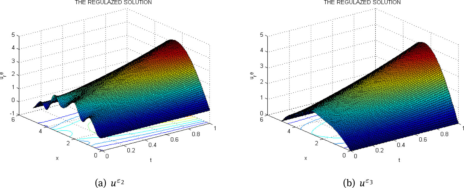
In this situation, the regularization parameter ε will be discussed. Fix α = 0.3, τ = 0.5. Consider ε1 = 10–1, ε2 = 10–3, ε3 = 10–5. We have the following figures:
For each point of time we evaluate the “Relative error” between the exact solution and the regularized solution which is defined by
The relative error is a better representation of the difference between the exact and the approximate solution. When the value of the exact solution is large, the difference between the exact and the approximate solution does not tell us much information about the accuracy of the approximation. In this case, the relative error is a better measurement. Figure 3 shows errors for a comparison between the exact solution and the regularized solution at the initial time t0 = 0 and τ = 1 with various values of ε. In Table 1, we have the error table at time time t* = 0.1.
The error and Relative error at time t* = 0.1.
| ∈ | ‖uε(., 0.1) – uex(., 0.1)‖ | RE(ε, 0.1) |
|---|---|---|
| ε1 = 10–1 | 2004.6002763324 | 40.0920055266479 |
| ε2 = 10–2 | 93.6668715963709 | 1.87333743192742 |
| ε3 = 10–3 | 11.7191083956268 | 0.234382i67912537 |
| ε4 = 10–4 | 0.333770043724429 | 0.0666754008744885 |
| ε5 = 10–5 | 0.0558155468882481 | 0.00111631093776496 |
Remark 3.1
From Figure 1, Figure 2, Figure 3, Figure 4 and Table 1, it is clear that as the mearsuring error ε gets smaller, the regularized solution gets closer and closer to the exact one. It is also noted that in this situation, the noise parameter cp varies from -249.689 to 242.4461.
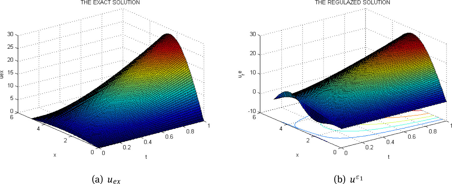
The exact solution with α = 0.3 (a) and regularized solution with ε1 = 10–1 (b)
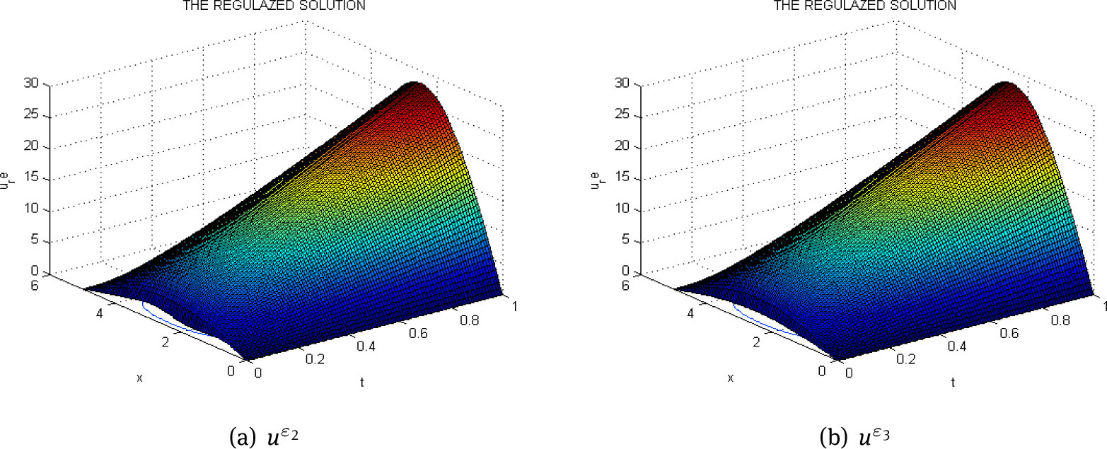
The regularized solution with ε2 = 10–3 (a) and with ε3 = 10–5 (b)
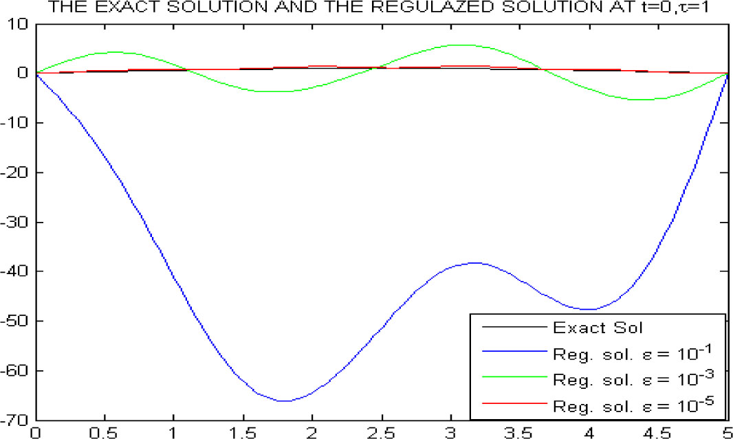
At time t0 = 0 and τ = 1: Exact solution with α = 0.9 (black) and Regularized solution with ε1 = 10–1 (blue), ε3 = 10–3 (green), ε5 = 10–5 (red)
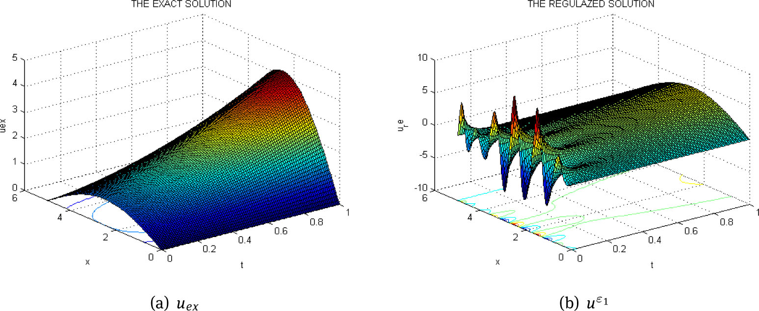
The exact solution with α = 0.1 (a) and regularized solution with ε1 = 10–1 (b)
The regularized solution with ε2 = 10–3 (a) and with ε3 = 10–5 (b)
In this situation, the focusing parameter is τ. Let α = 0.1 and fix ε = 10–3. Consider the series of τ: τ1 = 0.3, τ2 = 0.5, τ3 = 1. We have Figure 6 to illustrate our theoretical results. It is also noted that in this situation, the noise parameter cp varies from -220.5152 to 352.6678.
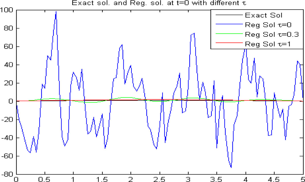
Case α = 0.5, At time t = 0 and ε1 = 10–3: Exact solution (black) and Regularized solution with τ1 = 0 (blue), τ2 = 0.3 (green), τ3 = 1 (red)
Remark 3.2
Figure 6 agrees with the theoretical result: the regularized solution with a higher value of τ is closer to the exact one. The parameter τ is very useful if we want to get a more accurate approximation if the measuring process cannot be improved or if the cost of measuring better is very expensive. In this case, with the appearance of τ, the error can be improved without any extra cost on measuring (as we can see in Figure 6).
4 Conclusion
In this paper, we have stated and discussed the quasi-boundary value regularization method for the inverse problem in the heat equation under the conformable derivative. In addition, we have also established an error estimate between exact and regularized solutions. These estimates are supported by several numerical examples. The estimate is a Hölder-type estimate (εt/T) for all values of t in the interval (0, T]. However, at the initial time t = 0, the error estimate is of logarithm type only. In the future, we hope to improve the error estimate as well as to consider the nonlinear case of f.
Competing interests: The authors declare that they have no competing interests.
Authors’ contributions: All authors contributed equally to the writing of this paper. All authors read and approved the final manuscript.
Acknowledgement
The authors are very grateful to the referees for their valuable suggestions, which helped to improve the paper significantly. The third author would like to thank Professor Dang Duc Trong, Associate Professor Nguyen Huy Tuan and Tra Quoc Khanh for their support.
References
[1] Tikhonov A.N., Arsenin V.Y., Solutions of ill-posed problems, Vh Winston, 1977.Search in Google Scholar
[2] Glasko V. B., Inverse problems of mathematical physics, New York: American Institute of Physics, 1984.Search in Google Scholar
[3] Denche M., Bessila K., A modified quasi-boundary value method for ill-posed problems, J. of Math. Anal. and Appl., 2005, 301 419-426.10.1016/j.jmaa.2004.08.001Search in Google Scholar
[4] Hao D.N., Duc N.V., Stability results for the heat equation backward in time, J. of Math. Anal. and Appl., 2009, 353, 627-641.10.1016/j.jmaa.2008.12.018Search in Google Scholar
[5] Hao D.N., Duc N.V., D. Lesnic, Regularization of parabolic equations backward in time by a non-local boundary value problem method, IMA J. of Appl. Math., 2010, 75, 291-315.10.1093/imamat/hxp026Search in Google Scholar
[6] Hao D.N., Duc N.V., Regularization of backward parabolic equations in Banach spaces, J. of Inverse. and Ill-posed Probs., 2012, 20, 745-763.10.1515/jip-2012-0046Search in Google Scholar
[7] Fu C.L., Qian Z., Shi R., A modified method for a backward heat conduction problem, Appl. Math. and Comput., 2007, 185, 564-573.10.1016/j.amc.2006.07.055Search in Google Scholar
[8] Fu C.L., Xiong X.T., Qian Z., Fourier regularization for a backward heat equation, J. Math. Anal. Appl., 2007, 331, 472-480.10.1016/j.jmaa.2006.08.040Search in Google Scholar
[9] Trong D.D., Quan P.H., Khanh T.V., Tuan N.H., A nonlinear case of the 1-D backward heat problem: Regularization and error estimate, Zeitschrift Analysis und ihre Anwendungen, 2007, 26, 231-245.10.4171/ZAA/1321Search in Google Scholar
[10] Trong D.D., Tuan N.H., Regularization and error estimate for the nonlinear backward heat problem using a method of integral equation, Nonlin. Anal.: Theo., Meth. and Appl., 2009, 71, 4167-4176.10.1016/j.na.2009.02.092Search in Google Scholar
[11] Trong D.D., Tuan N.H., Regularization and error estimate for the nonlinear backward heat problem using a method of integral equation, Nonlin. Anal.: Theo., Meth. and Appl., 2009, 71, 4167-4176.10.1016/j.na.2009.02.092Search in Google Scholar
[12] Magin R., Fractional calculus models of complex dynamics in biological tissues, Computers & Mathematics with Applications, 2010, 59, 1586-1593.10.1016/j.camwa.2009.08.039Search in Google Scholar
[13] Magin R., Ortigueira M., Podlubny I., Trujillo J.J., On the fractional signals and systems, Signal Processing, 2011, 91, 350-371.10.1016/j.sigpro.2010.08.003Search in Google Scholar
[14] Merala F.C., Roystona T.J., Magin R., Fractional calculus in viscoelasticity: An experimental study, Communications in Nonlinear Science and Numerical Simulation, 2010, 15, 939-945.10.1016/j.cnsns.2009.05.004Search in Google Scholar
[15] Samko S.G., Kilbas A.A., Marichev O.I., Fractional Integrals and Derivatives: Theory and Applications, Gordon and Breach Science Publishers, Switzerland, 1993.Search in Google Scholar
[16] Podlubny I., Fractional differential equation, San Diego: Academic Press, 1999.Search in Google Scholar
[17] Kilbas A.A., Srivastava H.M., Trujillo J.J., Theory and applications of fractional differential equations, Amesterdam: Elsevier Science B.V, 2006.Search in Google Scholar
[18] Atangana A., Baleanu D., New fractional derivatives with nonlocal and non-singular kernel: theory and application to heat transfer model, Thermal Science, 2016, 20, 763-769.10.2298/TSCI160111018ASearch in Google Scholar
[19] Atangana A., Koca I., Chaos in a simple nonlinear system with Atangana-Baleanu derivatives with fractional order, Chaos, Solitons & Fractals, 2016, 89, 447-454.10.1016/j.chaos.2016.02.012Search in Google Scholar
[20] Atangana A., Alkahtani B.S.T, Modeling the spread of Rubella disease using the concept of with local derivative with fractional parameter, Complexity, 21, 2015, 442-451.10.1002/cplx.21704Search in Google Scholar
[21] Atangana A., Alqahtani R.T., Delling the spread of river blindness disease via the caputo fractional derivative and the beta-derivative, Entropy, 18, 2016, 40. 10.3390/e18020040Search in Google Scholar
[22] Liu J.J., Yamamoto M., A backward problem for the time-fractional diffusion equation, Appl. Anal., 2010, 89, 1769-1788.10.1080/00036810903479731Search in Google Scholar
[23] Kenichi S., Yamamoto M., Initial value/boundary value problems for fractional diffusion-wave equations and applications to some inverse problem, Journal of Mathematical Analysis and Applications, 2011, 382 426-447.10.1016/j.jmaa.2011.04.058Search in Google Scholar
[24] Luchko Y., Some uniqueness and existence results for the initial-boundary-value problems for the generalized time-fractional diffusion equation., Comput. Math. Appl., 2010, 59 1766-1772.10.1016/j.camwa.2009.08.015Search in Google Scholar
[25] Jun-Gang W., Wei T., Zhou Y., Optimal error bound and simplified Tikhonov regularization method for a backward problem for the time-fractional diffusion equation, Journal of Computational and Applied Mathematics, 2015, 279, 277-292.10.1016/j.cam.2014.11.026Search in Google Scholar
[26] Tuan N.H., Nane E., Inverse source problem for time-fractional diffusion with discrete random noise, Statistics and Probability Letters, 2017, 120, 126-134.10.1016/j.spl.2016.09.026Search in Google Scholar
[27] Khalil R., Al Horani M., Yousef A., Sababheh M., A new Definition Of Fractional Derivative, J. Comput. Appl. Math., 2014, 264, 65-7010.1016/j.cam.2014.01.002Search in Google Scholar
[28] Atangana A., Baleanu D., Alsaedi A., New properties of conformable derivative, Open Mathematics, 2015, 13, 889-898.10.1515/math-2015-0081Search in Google Scholar
[29] Abdeljawad T., On conformable fractional calculus, J. Comput. Appl. Math., 2014, 279, 57-66.10.1016/j.cam.2014.10.016Search in Google Scholar
[30] Anderson D.R., Ulness D.J., Properties of the Katugampola fractional derivative with potential application in quantum mechanics, Journal of Mathematical Physics, 2015, 56, 063-50210.1063/1.4922018Search in Google Scholar
[31] Abu Hammad I., Khalil R.. Fractional Fourier Series with Applications, American Journal of Computational and Applied Mathematics, 2014, 4, 187-191.Search in Google Scholar
[32] Chung W.S., Fractional Newton mechanics with conformable fractional derivative, Journal of Computational and Applied Mathematics, 2015, 290, 150-158.10.1016/j.cam.2015.04.049Search in Google Scholar
[33] Eslami M., Exact traveling wave solutions to the fractional coupled nonlinear Schrodinger equations, Applied Mathematics and Computation, 2016, 285, 141-148.10.1016/j.amc.2016.03.032Search in Google Scholar
[34] Çenesiz Y., Baleanu D., Kurt A., Tasbozan O., New exact solutions of Burgers’ type equations with conformable derivative, Waves in Random and Complex Media, 2016, 1-14.10.1080/17455030.2016.1205237Search in Google Scholar
[35] Çenesiz Y., Kurt A., The solutions of time and space conformable fractional heat equations with conformable Fourier transform, Acta Universitatis Sapientiae, Mathematica, 2015, 7, 130-140.10.1515/ausm-2015-0009Search in Google Scholar
[36] Çenesiz Y., Kurt A., Nane E., Stochastic solutions of conformable fractional Cauchy problems, . arXiv preprint arXiv:1606.07010.10.1016/j.spl.2017.01.012Search in Google Scholar
© 2018 Vu et al., published by De Gruyter
This work is licensed under the Creative Commons Attribution-NonCommercial-NoDerivatives 4.0 License.
Articles in the same Issue
- Regular Articles
- Algebraic proofs for shallow water bi–Hamiltonian systems for three cocycle of the semi-direct product of Kac–Moody and Virasoro Lie algebras
- On a viscous two-fluid channel flow including evaporation
- Generation of pseudo-random numbers with the use of inverse chaotic transformation
- Singular Cauchy problem for the general Euler-Poisson-Darboux equation
- Ternary and n-ary f-distributive structures
- On the fine Simpson moduli spaces of 1-dimensional sheaves supported on plane quartics
- Evaluation of integrals with hypergeometric and logarithmic functions
- Bounded solutions of self-adjoint second order linear difference equations with periodic coeffients
- Oscillation of first order linear differential equations with several non-monotone delays
- Existence and regularity of mild solutions in some interpolation spaces for functional partial differential equations with nonlocal initial conditions
- The log-concavity of the q-derangement numbers of type B
- Generalized state maps and states on pseudo equality algebras
- Monotone subsequence via ultrapower
- Note on group irregularity strength of disconnected graphs
- On the security of the Courtois-Finiasz-Sendrier signature
- A further study on ordered regular equivalence relations in ordered semihypergroups
- On the structure vector field of a real hypersurface in complex quadric
- Rank relations between a {0, 1}-matrix and its complement
- Lie n superderivations and generalized Lie n superderivations of superalgebras
- Time parallelization scheme with an adaptive time step size for solving stiff initial value problems
- Stability problems and numerical integration on the Lie group SO(3) × R3 × R3
- On some fixed point results for (s, p, α)-contractive mappings in b-metric-like spaces and applications to integral equations
- On algebraic characterization of SSC of the Jahangir’s graph 𝓙n,m
- A greedy algorithm for interval greedoids
- On nonlinear evolution equation of second order in Banach spaces
- A primal-dual approach of weak vector equilibrium problems
- On new strong versions of Browder type theorems
- A Geršgorin-type eigenvalue localization set with n parameters for stochastic matrices
- Restriction conditions on PL(7, 2) codes (3 ≤ |𝓖i| ≤ 7)
- Singular integrals with variable kernel and fractional differentiation in homogeneous Morrey-Herz-type Hardy spaces with variable exponents
- Introduction to disoriented knot theory
- Restricted triangulation on circulant graphs
- Boundedness control sets for linear systems on Lie groups
- Chen’s inequalities for submanifolds in (κ, μ)-contact space form with a semi-symmetric metric connection
- Disjointed sum of products by a novel technique of orthogonalizing ORing
- A parametric linearizing approach for quadratically inequality constrained quadratic programs
- Generalizations of Steffensen’s inequality via the extension of Montgomery identity
- Vector fields satisfying the barycenter property
- On the freeness of hypersurface arrangements consisting of hyperplanes and spheres
- Biderivations of the higher rank Witt algebra without anti-symmetric condition
- Some remarks on spectra of nuclear operators
- Recursive interpolating sequences
- Involutory biquandles and singular knots and links
- Constacyclic codes over 𝔽pm[u1, u2,⋯,uk]/〈 ui2 = ui, uiuj = ujui〉
- Topological entropy for positively weak measure expansive shadowable maps
- Oscillation and non-oscillation of half-linear differential equations with coeffcients determined by functions having mean values
- On 𝓠-regular semigroups
- One kind power mean of the hybrid Gauss sums
- A reduced space branch and bound algorithm for a class of sum of ratios problems
- Some recurrence formulas for the Hermite polynomials and their squares
- A relaxed block splitting preconditioner for complex symmetric indefinite linear systems
- On f - prime radical in ordered semigroups
- Positive solutions of semipositone singular fractional differential systems with a parameter and integral boundary conditions
- Disjoint hypercyclicity equals disjoint supercyclicity for families of Taylor-type operators
- A stochastic differential game of low carbon technology sharing in collaborative innovation system of superior enterprises and inferior enterprises under uncertain environment
- Dynamic behavior analysis of a prey-predator model with ratio-dependent Monod-Haldane functional response
- The points and diameters of quantales
- Directed colimits of some flatness properties and purity of epimorphisms in S-posets
- Super (a, d)-H-antimagic labeling of subdivided graphs
- On the power sum problem of Lucas polynomials and its divisible property
- Existence of solutions for a shear thickening fluid-particle system with non-Newtonian potential
- On generalized P-reducible Finsler manifolds
- On Banach and Kuratowski Theorem, K-Lusin sets and strong sequences
- On the boundedness of square function generated by the Bessel differential operator in weighted Lebesque Lp,α spaces
- On the different kinds of separability of the space of Borel functions
- Curves in the Lorentz-Minkowski plane: elasticae, catenaries and grim-reapers
- Functional analysis method for the M/G/1 queueing model with single working vacation
- Existence of asymptotically periodic solutions for semilinear evolution equations with nonlocal initial conditions
- The existence of solutions to certain type of nonlinear difference-differential equations
- Domination in 4-regular Knödel graphs
- Stepanov-like pseudo almost periodic functions on time scales and applications to dynamic equations with delay
- Algebras of right ample semigroups
- Random attractors for stochastic retarded reaction-diffusion equations with multiplicative white noise on unbounded domains
- Nontrivial periodic solutions to delay difference equations via Morse theory
- A note on the three-way generalization of the Jordan canonical form
- On some varieties of ai-semirings satisfying xp+1 ≈ x
- Abstract-valued Orlicz spaces of range-varying type
- On the recursive properties of one kind hybrid power mean involving two-term exponential sums and Gauss sums
- Arithmetic of generalized Dedekind sums and their modularity
- Multipreconditioned GMRES for simulating stochastic automata networks
- Regularization and error estimates for an inverse heat problem under the conformable derivative
- Transitivity of the εm-relation on (m-idempotent) hyperrings
- Learning Bayesian networks based on bi-velocity discrete particle swarm optimization with mutation operator
- Simultaneous prediction in the generalized linear model
- Two asymptotic expansions for gamma function developed by Windschitl’s formula
- State maps on semihoops
- 𝓜𝓝-convergence and lim-inf𝓜-convergence in partially ordered sets
- Stability and convergence of a local discontinuous Galerkin finite element method for the general Lax equation
- New topology in residuated lattices
- Optimality and duality in set-valued optimization utilizing limit sets
- An improved Schwarz Lemma at the boundary
- Initial layer problem of the Boussinesq system for Rayleigh-Bénard convection with infinite Prandtl number limit
- Toeplitz matrices whose elements are coefficients of Bazilevič functions
- Epi-mild normality
- Nonlinear elastic beam problems with the parameter near resonance
- Orlicz difference bodies
- The Picard group of Brauer-Severi varieties
- Galoisian and qualitative approaches to linear Polyanin-Zaitsev vector fields
- Weak group inverse
- Infinite growth of solutions of second order complex differential equation
- Semi-Hurewicz-Type properties in ditopological texture spaces
- Chaos and bifurcation in the controlled chaotic system
- Translatability and translatable semigroups
- Sharp bounds for partition dimension of generalized Möbius ladders
- Uniqueness theorems for L-functions in the extended Selberg class
- An effective algorithm for globally solving quadratic programs using parametric linearization technique
- Bounds of Strong EMT Strength for certain Subdivision of Star and Bistar
- On categorical aspects of S -quantales
- On the algebraicity of coefficients of half-integral weight mock modular forms
- Dunkl analogue of Szász-mirakjan operators of blending type
- Majorization, “useful” Csiszár divergence and “useful” Zipf-Mandelbrot law
- Global stability of a distributed delayed viral model with general incidence rate
- Analyzing a generalized pest-natural enemy model with nonlinear impulsive control
- Boundary value problems of a discrete generalized beam equation via variational methods
- Common fixed point theorem of six self-mappings in Menger spaces using (CLRST) property
- Periodic and subharmonic solutions for a 2nth-order p-Laplacian difference equation containing both advances and retardations
- Spectrum of free-form Sudoku graphs
- Regularity of fuzzy convergence spaces
- The well-posedness of solution to a compressible non-Newtonian fluid with self-gravitational potential
- On further refinements for Young inequalities
- Pretty good state transfer on 1-sum of star graphs
- On a conjecture about generalized Q-recurrence
- Univariate approximating schemes and their non-tensor product generalization
- Multi-term fractional differential equations with nonlocal boundary conditions
- Homoclinic and heteroclinic solutions to a hepatitis C evolution model
- Regularity of one-sided multilinear fractional maximal functions
- Galois connections between sets of paths and closure operators in simple graphs
- KGSA: A Gravitational Search Algorithm for Multimodal Optimization based on K-Means Niching Technique and a Novel Elitism Strategy
- θ-type Calderón-Zygmund Operators and Commutators in Variable Exponents Herz space
- An integral that counts the zeros of a function
- On rough sets induced by fuzzy relations approach in semigroups
- Computational uncertainty quantification for random non-autonomous second order linear differential equations via adapted gPC: a comparative case study with random Fröbenius method and Monte Carlo simulation
- The fourth order strongly noncanonical operators
- Topical Issue on Cyber-security Mathematics
- Review of Cryptographic Schemes applied to Remote Electronic Voting systems: remaining challenges and the upcoming post-quantum paradigm
- Linearity in decimation-based generators: an improved cryptanalysis on the shrinking generator
- On dynamic network security: A random decentering algorithm on graphs