Univariate approximating schemes and their non-tensor product generalization
-
 and
and

Abstract
This article deals with univariate binary approximating subdivision schemes and their generalization to non-tensor product bivariate subdivision schemes. The two algorithms are presented with one tension and two integer parameters which generate families of univariate and bivariate schemes. The tension parameter controls the shape of the limit curve and surface while integer parameters identify the members of the family. It is demonstrated that the proposed schemes preserve monotonicity of initial data. Moreover, continuity, polynomial reproduction and generation of the schemes are also discussed. Comparison with existing schemes is also given.
1 Introduction
One of the important areas of study in Computer Aided Geometric Design is subdivision. Subdivision schemes have become very important for providing smooth curves and surfaces through an iterative process from a finite set of control points. At each step of iteration, a new set of points is created from the old points. In general, approximating subdivision schemes produce smoother curves and surfaces as compared to interpolating subdivision schemes.
Approximating schemes were first developed by Rham [1]. A famous corner cutting linear approximation scheme was introduced by Chaikin [2], which can generate the piecewise continuous C1 limiting curves. Consequent to this, a lot of work has been done by different authors in the area of binary approximating subdivision schemes. Mustafa et al. [3] presented the m-point binary approximating subdivision scheme. Zheng et al. [4] introduced a general formula to generate a family of integer-point binary approximating sub-division schemes with a parameter. Mustafa et al. [5] presented a family of (2n−1)-point binary approximating subdivision schemes with free parameters for describing curves. Khan and Mustafa [6] introduced a new approach to construct a non-tensor product C1 subdivision scheme for quadrilateral meshes. Zheng et al. [7] devised a multi-parameter method which generates a class of existing binary subdivision schemes. By using their method continuity of existing schemes can be increased up to Ck+n by multiplying the factor
Lane and Riesenfeld [8] then presented a unified framework to represent the uniform B-spline curves and their tensor product extensions by a subdivision process. This framework consists of two stages, the first
stage doubles the control point by taking each point twice and the second stage is the midpoint averaging of these points.
Cashman et al. [9] presented the generalized Lane-Riesenfeld algorithm with 4-point variant. A subdivision step T is therefore
where R is refine stage and S is smoothing stage.
Ashraf et al. [10] applied a six point variant on the Lane-Riesenfeld algorithm to generate a family of subdivision schemes by defining
where Wq is refine stage and Sq is smoothing stage.
Hormann and Sabin [11] proposed a family of subdivision schemes with symbol ak(z) by convolution of uniform B-spline with kernel given by
where σ(z) is a smoothing operator of the B-spline and Kk(z) is a convolution of the order-k B-spline with the kernel.
Conti and Romani [12] proposed a strategy for constructing dual m-ary approximating subdivision schemes of de Rham-type, starting from two primal schemes of arity m and 2 respectively. Symbol of their scheme is
where aodd(z) is the odd sub-symbol of a primal binary scheme and b(z) is the symbol of a primal m-ary scheme. Mustafa et al. [13] presented an algorithm that generates a family of binary univariate dual and primal approximating subdivision schemes, starting with two binary schemes, defined as
where meven(z) is the even sub-symbol of [14] and n(z) is the symbol of [11]. Romani [15] introduced an algorithm which generates the univariate and bivariate non-tensor product subdivision schemes with tension parameter. The symbol of the scheme is defined as
where
1.1 Motivation
All the above algorithms are also called Refine-Smooth algorithms. In these algorithms there is one smoothing operator followed by one refining operator. But in the proposed algorithm there are two smoothing operators followed by one refining operator. That is, we propose an algorithm which uses symbols of well known subdivision schemes, starting with three binary schemes i.e.
where αodd(z) is the extracted odd sub-symbol of [4], βeven(z) is the extracted even sub-symbol of [14] and γμ(z) is the symbol of [5]. The schemes produced by this algorithm are continuous up to Cm+n+2, where m and n are parameters that identify members of the family and play a crucial role in the continuity of the proposed schemes. The parameter μ controls the shape of the limit curves of the schemes. Moreover, this algorithm produces higher order continuous schemes compared with to the existing algorithms. This algorithm can easily be generalized to produce non-tensor product binary approximating schemes for surface generation. Furthermore, monotonicity preservation is also an important shape preserving property of subdivision schemes. In [16, 17, 18, 19, 20, 21] the monotonicity of univariate schemes has been discussed. In this paper, we examine monotonicity preservation of univariate schemes and non-tensor product schemes.
The remainder of this article is organized into 3 sections. In Section 2, firstly we present an algorithm which generates a family of univariate binary approximating subdivision schemes with a tension parameter. Secondly, we discuss the smoothness analysis of univariate schemes and finally we discuss the monotonicity, polynomial generation and reproduction of the schemes. Section 3 extends the ideas presented in Section 2 to design a new family of non-tensor product subdivision schemes for quadrilateral meshes. The smoothness analysis of non-tensor product schemes is also discussed in the same section. In Section 3, we also discuss the monotonicity, polynomial generation and reproduction properties of non-tensor product subdivision schemes. Applications and conclusion are also given in this section.
2 Algorithm for univariate schemes
In this section, we present an algorithm for the construction of a family of binary approximating subdivision schemes.
For this, we consider the odd sub-symbol of cubic B-spline scheme [4]
Similarly, the even sub-symbol of 4-point binary interpolating scheme [14] is
The symbol of the three point scheme [5] is given by
Let us denote the family of the binary approximating subdivision scheme by Pqm,n,μ, where the general member of the proposed family has the symbol of the form
Substituting (1), (2) and (3) in (4), we get the symbol of the scheme Pqm,n,μ
where m and n are non-negative integers. As it is apparent that the symbol of the scheme Pqm,n,μ is dependent on the parameter μ and on two other parameters m and n. The parameter μ controls the shape of the limit curves of the schemes while m and n characterize the elements of the scheme Pqm,n,μ.
2.1 Smoothness analysis of univariate schemes
In this section, we discuss the continuity and Hölder continuity of the schemes. We use the theory of generating function [22] for continuity and Rioul’s [23] method for Hölder continuity. In the following theorem, we examine the convergence and smoothness of the scheme Pqm,0,μ.
Theorem 2.1
The schemePqm,0,μis Cm+2for μ ϵ (0, 0.125).
Proof. Symbol of the scheme Pqm,0,μ is given by
where
and
Let Sb be the scheme corresponding to the symbol b(z). Since
then for μ ϵ (0, 0.125), we have
Hence Sb is contractive. Therefore, by Corollary 4.11 of [22], the scheme Sa is C2 for μ ϵ (0, 0.125). So by (6) scheme Pqm,0,μ is Cm+2 for μ ϵ (0, 0.125).
Similarly, we can easily find out the continuity of other schemes Pqm,n,μ by taking into account the same formalism. The order of continuity of some proposed univariate subdivision schemes Pqm,0,μ , Pqm,1,μ , Pqm,2,μ and Pqm,3,μ for certain ranges of parameter is shown in Table 1. Hölder continuity is an extension to the notion of continuity. In the following theorem, we compute the Hölder continuity of the scheme Pqm,0,μ.
The order of continuity O(C) of proposed binary approximating schemes for certain ranges of parameter.
| n | Scheme | Ranges | O(C) | n | Scheme | Ranges | O(C) |
|---|---|---|---|---|---|---|---|
| 0 | Pqm,0,μ | −0.375 < μ < 0.625 | Cm+0 | 2 | Pqm,2,μ | −0.195 < μ < 0.445 | Cm+0 |
| ... | −0.125 < μ < 0.375 | Cm+1 | ... | −0.194 < μ < 0.442 | Cm+1 | ||
| ... | 0 < μ < 0.125 | Cm+2 | ... | −0.034 < μ < 0.282 | Cm+2 | ||
| ... | −0.026 < μ < 0.235 | Cm+3 | |||||
| ... | 0.045 < μ < 0.09 | Cm+4 | |||||
| 1 | Pqm,1,μ | −0.275 < μ < 0.525 | Cm+0 | 3 | Pqm,3,μ | −0.356 < μ < 0.618 | Cm+0 |
| ... | −0.075 < μ < 0.3 | Cm+1 | ... | −0.131 < μ < 0.380 | Cm+1 | ||
| ... | −0.068 < μ < 0.295 | Cm+2 | ... | −0.128 < μ < 0.375 | Cm+2 | ||
| ... | 0.025 < μ < 0.104 | Cm+3 | ... | −0.002 < μ < 0.235 | Cm+3 | ||
| ... | 0.003 < μ < 0.191 | Cm+4 | |||||
| ... | 0.006 < μ < 0.081 | Cm+5 |
Theorem 2.2
The Hölder continuity of the schemePqm,0,μis 3.
Proof. From (7), let b0 = 8μ, b1 = 2 − 16μ, b2 = 8μ, then M0, M1 are the matrices with elements
where i, j = 1, 2. This implies
From (8) and [23], the spectral radius λ of the metrics M0 and M1 can be express as follows
Since the largest eigenvalue and the max-norm of the metrics is 1 for μ = 0.0625, where μ ϵ (0, 0.125), so the Hölder continuity h = 2 − log2(1) = 3. So by (6), the Hölder continuity of the scheme Pqm,0,μ is Cm+3.
Similarly, we can compute the Hölder continuity of other members of the family. If the largest eigenvalue and the max-norm of the metrics are not equal then we calculate the lower and upper bounds of the Hölder continuity. The lower bound of the Hölder continuity is h = 2 − log2(kbkl)/l for some integer l and the upper bound of the Hölder continuity is h = 2 − log2(λ). It is clear from Table 2 that as we increase n, the level of continuity and the Hölder continuity of the schemes Pqm,n,μ increase.
Continuity of some members of the family of schemes
| n | μ | Continuity | Lower bound on Hölder continuity | Upper bound on Hölder continuity |
|---|---|---|---|---|
| 0 | 0.0625 | Cm+2 | Cm+3 | Cm+3 |
| 1 | 0.0375 | Cm+3 | Cm+3.255 | Cm+3.2603 |
| 2 | 0.0676 | Cm+3 | Cm+4.478 | Cm+5 |
2.2 Response of univariate schemes to polynomial and monotone data
In this section, we examine the response of schemes to polynomial data by taking into account the polynomial generation and reproduction. We also examine the behaviour of the schemes for monotone data. We use the techniques developed in [15] to discuss polynomial generation and polynomial reproduction.
2.2.1 Polynomial generation
The polynomial generation of degree d is the ability of subdivision scheme to generate the full space of polynomials up to degree d denoted by πd. The generation degree of a subdivision scheme is the maximum degree of a polynomial that can potentially be generated by the scheme.
Theorem 2.3
The subdivision schemePqm,n,μgenerates πm+n+2for all m, n ϵ N. Moreover, if
Proof. Since conditions
are verified by qm,n,μ(z) for all μ ϵ ℝ and D(k) denotes the kth derivative. Thus, in view of Proposition 2.1 of [15] degree of polynomial generation is m + n + 2 for all μ ϵ ℝ. Moreover, by setting
2.2.2 Polynomial reproduction
Polynomial reproduction is an attractive property for a subdivision scheme. For a subdivision scheme to reproduce πd it must be able to generate polynomials of the same degree as the limit functions for some initial data. The degree of polynomial reproduction can never exceed the degree of polynomial generation.
Theorem 2.4
If applying the parameter shift
Proof. Since the condition D(1)qm,n,μ(1) = 5 + m + 3n is verified by the symbol qm,n,μ(z) for all μ ϵ ℝ, so polynomial reproduction of Pqm,n,μ is π1 with the parameter shift
are satisfied for all m, n ϵ ℕ. Thus reproduction of Pqm,n,μ is π3.
2.3 Monotonicity preservation
Monotonicity preserving plays a key role in the shape preserving properties of subdivision schemes.
Definition 2.1
[18] Univariate data (xi , fi), i = 0, 1, 2, . . . , n is monotonically increasing if fi < fi+18 i = 0, 1, 2, . . . , n and the derivative at the data points obey the condition di > 0 ∀ i = 0, 1, 2, . . . , n.
In the following, we examine monotonicity preservation of binary scheme Pq1,0,μ.
Theorem 2.5
Let
Denote
Furthermore, let 0.1 ≤ μ ≤ 0.9 and
Proof. We use mathematical induction to prove (9). When k = 0,
Suppose that (9) holds for
This implies
This further implies
We know that
This implies that
then
The denominator and numerator of the right hand side of the above expression are less than and greater than zero respectively for 0.1 ≤ μ ≤ 0.9 and
This implies that
It implies further that
This implies
The denominator and numerator of the right hand side of the above expression are less than and greater than zero respectively for 0.1 ≤ μ ≤ 0.9 and
This implies that
It implies further that
2.4 Numerical experiments of univariate schemes
In this section, we present the performance, geometrical behaviour and effect of a parameter on the limit curves of the schemes. We also present the response of the limit curves produced by the schemes towards the initial data.
Figure 1 is produced by using the monotone data set given in Table 3. Figures 1(a)-1(d) are monotone curves obtained by the schemes Pq1,0,μ , Pq1,1,μ , Pq1,2,μ and Pq1,3,μ respectively.
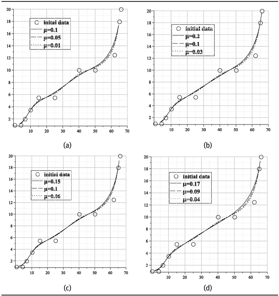
The curves (a), (b), (c) and (d) are generated by the schemes Pq1,0,μ , Pq1,1,μ , Pq1,2,μ and Pq1,3,μ respectively, using the monotone data set given below.
Monotone data set [24].
| i | 1 | 2 | 3 | 4 | 5 | 6 | 7 | 8 | 9 | 10 | 11 |
|---|---|---|---|---|---|---|---|---|---|---|---|
| xi | 0.1 | 4 | 6.5 | 10 | 15 | 25 | 40 | 50 | 62 | 65 | 66 |
| yi | 1 | 1 | 2 | 3.5 | 5.5 | 5.5 | 10 | 10 | 12.5 | 18 | 20 |
The Figure 2, 3, 4, 5 shows a comparison of proposed schemes with existing schemes [15]. Dashed dotted lines indicate the initial polygon. Solid lines show the most expanded curves and dashed lines show the most shrinked curves. Arrows show the distance between most expanded and most shrinked curves. Figures 2(a)-2(c) show that the most expanded and most shrinked curves are obtained by the schemes Pq2,0,μ , Pq1,2,μ and Pq2,2,μ at different parametric values and Figure 2(d) shows the behaviour of existing scheme of [15]. We can see that the Figures 3(a)-3(b) represent the interpolating behaviour of proposed scheme Pq2,0,μ , Pq1,2,μ respectively. Figure 3(c) shows the non-interpolating behaviour of [15] at any parametric value. The proposed schemes Pq2,0,μ and Pq1,2,μ show the approximating behaviour as well as the interpolating behaviour at different parametric values.
![Figure 2 Most expanded and most shrinked curves: The curves (a), (b), (c) and (d) are generated by the schemes Pq2,0,μ , Pq1,2,μ, Pq2,2,μ and [15] respectively.](/document/doi/10.1515/math-2018-0126/asset/graphic/j_math-2018-0126_fig_002.jpg)
Most expanded and most shrinked curves: The curves (a), (b), (c) and (d) are generated by the schemes Pq2,0,μ , Pq1,2,μ, Pq2,2,μ and [15] respectively.
![Figure 3 Interpolating behaviour: The curves (a) , (b) and (c) are generated by the schemes Pq2,0,μ , Pq1,2,μ and [15] respectively.](/document/doi/10.1515/math-2018-0126/asset/graphic/j_math-2018-0126_fig_003.jpg)
Interpolating behaviour: The curves (a) , (b) and (c) are generated by the schemes Pq2,0,μ , Pq1,2,μ and [15] respectively.
![Figure 4 Most expanded and most shrinked curves: The curves (a), (b) and (c) are generated by the schemes Pq1,0,μ , Pq1,1,μ and [15] respectively.](/document/doi/10.1515/math-2018-0126/asset/graphic/j_math-2018-0126_fig_004.jpg)
Most expanded and most shrinked curves: The curves (a), (b) and (c) are generated by the schemes Pq1,0,μ , Pq1,1,μ and [15] respectively.
![Figure 5 Interpolating behaviour: The curves (a), (b) and (c) are generated by the schemes Pq1,0,μ , Pq1,1,μ and [15] respectively.](/document/doi/10.1515/math-2018-0126/asset/graphic/j_math-2018-0126_fig_005.jpg)
Interpolating behaviour: The curves (a), (b) and (c) are generated by the schemes Pq1,0,μ , Pq1,1,μ and [15] respectively.
The Figures 4(a)-4(c) show the most expanded and most shrinked curves that are generated by the schemes Pq1,0,μ , Pq1,1,μ and [15] at different parametric values respectively. The limit curves presented in Figures 5(a)-5(c) show the interpolating behaviour by of schemes Pq1,0,μ , Pq1,1,μ and [15] respectively. The schemes Pq1,0,μ and Pq1,1,μ have both approximating and interpolating behaviour while the scheme in [15] gives only interpolating behaviour.
3 Algorithm for non-tensor product schemes
By generalizing the algorithm as devised in Section 2, we get a family of non-tensor product approximating schemes with tension parameter μ for quadrilateral meshes. Let Pqm,n,μ be the family of non-tensor product bivariate subdivision schemes then we propose the symbol of this family as
By substituting m = 1 and n = 0 in (10), we get symbol of the scheme Pq1,0,μ as follows:
The bivariate subdivision scheme Pq1,0,μ has the mask
3.1 Smoothness analysis of bivariate proposed schemes
Here, we use the theory of generating function [22] to derive continuity of non-tensor product schemes.
Theorem 3.1
If μ ϵ (−0.2215, 0.4785) then the subdivision schemePq1,0,μconverges to a continuous surface when starting from any regular quadrilateral mesh. Moreover, if μ ϵ (−0.05178, 0.3017) and μ ϵ (−0.0517, 0.25), then the limit surfaces generated by schemePq1,0,μhave C1and C2-continuity respectively.
Proof. From (11), we have
In view of [22](Theorem 4.30), we can determine the range of the parameter μ which guarantees the convergence of the scheme Pq1,0,μ by checking the contractivity of the scheme. Since the scheme with symbol
Again since, the scheme with symbol
b1,0,μ(z1, z2) is contractive for μ ϵ (−0.0517, 0.25), so the scheme Pq1,0,μ is C-continuous.
In Table 4, we compare the continuity of proposed non-tensor product schemes with some existing binary non-tensor product schemes. It is observed that the continuity of proposed schemes is better than the continuity of existing schemes.
The order of continuity O(C) of proposed non-tensor product schemes with some existing non-tensor product schemes.
| Scheme | Type | O(C) |
|---|---|---|
| Binary non-tensor product [15] | Interpolating | C1 |
| Binary non-tensor product [15] | Approximating | C1 |
| Binary non-tensor product [6] | Approximating | C1 |
| Proposed binary non-tensor product Pq1,0,μ | Approximating | C2 |
| Proposed binary non-tensor product Pq1,1,μ | Approximating | C3 |
3.2 Response of non-tensor product schemes to polynomial and monotone data
In this section, we investigate the capability of the non-tensor product approximating subdivision schemes Pq1,0,μ and Pq1,1,μ of generating and reproducing polynomials as well as monotonicity preservation of the data.
Theorem 3.2
The subdivision schemePq1,0,μgenerates π2for all μ ϵ ℝ and generates π4for
Proof. Let w1 = (1, −1), w2 = (−1, 1), w3 = (−1, −1) and let Dj with j ϵ ℕ2, denote a directional derivative. Since q1,0,μ(1, 1) = 4 and
then scheme Pq1,0,μ generates π1 for all μ ϵ ℝ. Again since
then the scheme Pq1,0,μ generates π2 for all μ ϵ ℝ. Further
so the scheme Pq1,0,μ generates π3 for
so the scheme Pq1,0,μ generates π4 for
Theorem 3.3
For the parameter shift
Proof. Let Dj with j ϵ ℕ2, denote a directional derivative. Since the symbol q1,0,μ(z1, z2) satisfies the conditions in Theorem 3.2. Since q1,0,μ(1, 1) = 4 and
then the scheme Pq1,0,μ produced π1 for all μ ϵ ℝ.
Similarly, we can prove the following theorems.
Theorem 3.4
The subdivision schemePq1,1,μgenerates π3for all μ ϵ ℝ and generates π4for
Theorem 3.5
If applying the parameteric shift (τ1, τ2) = (3, 4), the subdivision schemePq1,1,μreproduces π1with respect to the parametrization in [15] for all μ ϵ ℝ.
Now, we examine monotonicity preservation of the binary non-tensor product approximating subdivision scheme Pq1,0,μ.
Definition 3.1
[18] Bivariate data (xi , yj , fi,j), i = 0, 1, 2, . . . , n and j = 0, 1, 2, . . . , m, where x1 < x2 < . . . < xn and y1 < y2 < . . . < ym are said to be monotonically increasing if fi,j < fi+1,j and fi,j < fi,j+18 i = 0, 1, 2, . . . , n and j = 0, 1, 2, . . . , m, if the derivative at the data points obey the condition di,j > 0 8 i = 0, 1, 2, . . . , n and j = 0, 1, 2, . . . , m.
Theorem 3.6
Suppose that the initial data
Denote
Furthermore, let 0.1 ≤ μ ≤ 0.9 and
Proof. We use mathematical induction to prove (13). When
Suppose that (13) holds for k i.e.
First we show that
After some simplification and substituting
We know that
This implies that
Now we prove that
For this, consider
After some simplification and substituting
where
and
The denominator and numerator of the right hand side of the above expression are less than and greater than zero respectively for 0.1 ≤ μ ≤ 0.9. This implies that
Further this implies that
For this, consider
After some simplification and substituting
where
and
The denominator and numerator of the right hand side of the above expression are greater than and less than zero respectively for 0.1 ≤ μ ≤ 0.9. This implies that
Further this implies that
3.3 Numerical experiments of non-tensor product schemes
In this section, we show the performance, geometrical behaviour and effect of a parameter on the limit surfaces of the schemes Pq1,0,μ and Pq1,1,μ.
The monotone data set given in Table 5 has been used to produce monotone surfaces. Figure 6(a) is the initial mesh of the monotone data. Figure 6(b) is the monotone surface generated by the scheme Pq1,0,μ for μ = 0.5. Figure 7(a) is the initial control mesh while Figures 7(b)-7(d) are the surfaces produced by the proposed scheme Pq1,0,μ at first, second and third subdivision levels with μ = 0.1 respectively. Figure 8(a) is the initial control mesh while Figures 8(b), Figures 8(c), 8(d) are the surfaces produced by the proposed scheme Pq1,1,μ at first, second and third subdivision levels with μ = 0.15 respectively.
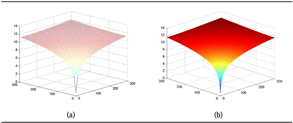
(a) Initial monotone data. (b) A monotonicity preserving surface obtained by the proposed scheme Pq1,0,μ.
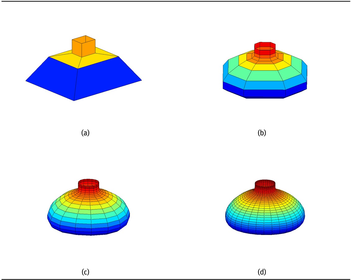
(a) Control mesh. (b)-(d) Surfaces obtained by the proposed schemes Pq1,0,μ at first, second and third subdivision levels respectively.
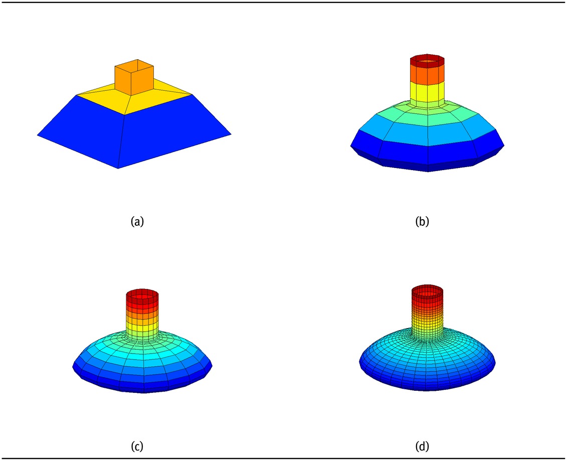
(a) Control mesh. (b)-(d) Surfaces obtained by the proposed schemes Pq1,1,μ at first, second and third subdivision levels respectively.
Monotone data set [25].
| x/y | 1 | 100 | 200 | 300 |
|---|---|---|---|---|
| 1 | 0.6931 | 9.2104 | 10.5967 | 11.4076 |
| 100 | 9.2104 | 9.9035 | 10.8198 | 11.5129 |
| 200 | 10.5967 | 10.8198 | 11.2898 | 11.7753 |
| 300 | 11.4076 | 11.5129 | 11.7753 | 12.1007 |
3.4 Conclusion
In this paper, we have proposed two algorithms to generate the families of univariate and bivariate approximating subdivision schemes with one tension and two integer parameters. The integer parameters identify
members of the proposed family. It has been shown that the proposed schemes have higher continuity and Hölder continuity compared with existing schemes. Comparison of the continuity of proposed non-tensor product schemes with some of the existing non-tensor schemes has also been given. It has been demonstrated through several examples that geometrical behaviour of the univariate and bivariate subdivision schemes depends on the tension parameter. Monotonicity preservation of proposed univariate and bivariate schemes has been proved. Moreover, polynomial reproduction and generation of the proposed schemes have also been discussed.
Acknowledgement
This work is supported by the Indigenous Ph.D. Scholarship Scheme of Higher Education Commission (HEC) Pakistan and NRPU No-3183
References
[1] Rham G. de, Un peude Mathematiques a proposed’ une courbe plane, Revwe de Mathematiques elementry II, Oevred Compl., 1947, 678-689Search in Google Scholar
[2] Chaikin G. M., An algorithm for high speed curve generation, Comp. Graph. Imag. Proces., 1974, 3, 346-34910.1016/0146-664X(74)90028-8Search in Google Scholar
[3] Mustafa G., Khan F. and Ghaffar A., The m-point approximating subdivision scheme, Lobachevskii J.Math., 2009, 30, 138-14510.1134/S1995080209020061Search in Google Scholar
[4] Zheng H., Huang S., Guo F. and Peng G., Integer-point binary approximating subdivision schemes, J. Info. Comput. Sci., 2014, 10, 3387-339810.12733/jics20104000Search in Google Scholar
[5] Mustafa G. , Ghaffar A. and Bari M., (2n-1)-point binary approximating scheme, Digital Information Management (ICDIM), International Conference, 363-368 (2013)10.1109/ICDIM.2013.6694036Search in Google Scholar
[6] Khan F. and Mustafa G., A new non-tensor product C1 subdivision scheme for regular quad meshes, World Appl. Sci. J., 2013, 24, 1635-1641Search in Google Scholar
[7] Zheng H. C., Huang S. C., Guo F. and Peng G. H., Designing multi-parameter curve subdivision schemes with high continuity, Appl. Math. Comput., 2014, 243, 197-20810.1016/j.amc.2014.05.113Search in Google Scholar
[8] Lane J. M. and Riesenfeld R. F., A theoretical development for computer generation and display of piecewise polynomial surfaces, IEEE Tran. Patt. Anal. Mach. Intel., 1980, 2, 35-4610.1109/TPAMI.1980.4766968Search in Google Scholar PubMed
[9] Cashman T. J., Hormann K. and Reif U., Generalized Lane-Riesenfeld algorithms, Comp. Aid. Geomet. Des., 2013, 30, 398-40910.1016/j.cagd.2013.02.001Search in Google Scholar
[10] Ashraf P., Mustafa G. and Deng J., A six-point variant on the Lane-Riesenfeld algorithm, J. Appl. Math., 2014, 1-710.1155/2014/628285Search in Google Scholar
[11] Hormanm K. and Sabin M., A family of subdivision schemes with cubic precision, Comp. Aid. Geomet. Des., 2008, 25, 41-5210.1016/j.cagd.2007.04.002Search in Google Scholar
[12] Conti C. and Romani L., Dual univariate m-ary subdivision schemes of de Rham-type, J.Math. Anal. Appl., 2013, 407, 443-45610.1016/j.jmaa.2013.05.009Search in Google Scholar
[13] Mustafa G., Ashraf P. and Aslam M., Binary univariate dual and primal subdivision schemes, SeMA, 2014, 65, 23-3510.1007/s40324-014-0017-6Search in Google Scholar
[14] Dyn N., Levin D. and Gregory J. A., A 4-point interpolatory subdivision scheme for curve design, Comp. Aid. Geomet. Des., 1987, 4, 257-26810.1016/0167-8396(87)90001-XSearch in Google Scholar
[15] Romani L., A Chaikin-based variant of Lane-Riesenfeld algorithm and its non-tensor product extension, Comp. Aid. Geomet. Des., 2015, 32, 22-4910.1016/j.cagd.2014.11.002Search in Google Scholar
[16] Cai Z., Convergence, error estimation and some properties of four-point interpolation subdivision scheme, Comp. Aid. Geomet. Des., 1995, 12, 459-46810.1016/0167-8396(94)00024-MSearch in Google Scholar
[17] Hussan M. Z. and Hussan M., Visualization of data preserving monotonicity, Appl. Math. Comput., 2007, 190, 1353-136410.1016/j.amc.2007.02.022Search in Google Scholar
[18] Hussan M. Z., Sarfraz M. and Shaikh T. S., Monotone data visualization using rational functions, World Appl. Sci. J., 2012, 16, 1496-1508Search in Google Scholar
[19] Kuijt F. and Damme R. V., Monotonicity preserving interpolatory subdivision schemes, J. Comput. Appl. Math., 1999, 101, 203-22910.1016/S0377-0427(98)00220-9Search in Google Scholar
[20] Shalom Y., Monotonicity preserving subdivision scheme, J. Approx. Theo., 1993, 74, 41-5810.1006/jath.1993.1052Search in Google Scholar
[21] Tan J., Zhuang X. and Zhang L., A new four-point shape-preserving C3 subdivision scheme, Comp. Aid. Geomet. Des., 2014, 31, 57-6210.1016/j.cagd.2013.12.003Search in Google Scholar
[22] Dyn N. and Levin D., Subdivision schemes in the geometric modelling, Act. Numer., 2002, 11, 73-14410.1017/S0962492902000028Search in Google Scholar
[23] Rioul O., Simple regularity for subdivision schemes, SIAM J. Math. Anal., 1992, 23, 1544-157610.1137/0523086Search in Google Scholar
[24] Abbas M., Majid A. A., Awang M. N. H. and Ali J. M., Monotonicity-preserving rational bi-cubic spline surface interpolation, Sci. Asia, 2014, 40S, 22-3010.2306/scienceasia1513-1874.2014.40S.022Search in Google Scholar
[25] Hussain M. Z. and Hussain M., Visualization of data preserving monotonicity, Appl. Math. Comput., 2007, 190, 1353-136410.1016/j.amc.2007.02.022Search in Google Scholar
© 2018 Mustafa and Bashir, published by De Gruyter
This work is licensed under the Creative Commons Attribution-NonCommercial-NoDerivatives 4.0 License.
Articles in the same Issue
- Regular Articles
- Algebraic proofs for shallow water bi–Hamiltonian systems for three cocycle of the semi-direct product of Kac–Moody and Virasoro Lie algebras
- On a viscous two-fluid channel flow including evaporation
- Generation of pseudo-random numbers with the use of inverse chaotic transformation
- Singular Cauchy problem for the general Euler-Poisson-Darboux equation
- Ternary and n-ary f-distributive structures
- On the fine Simpson moduli spaces of 1-dimensional sheaves supported on plane quartics
- Evaluation of integrals with hypergeometric and logarithmic functions
- Bounded solutions of self-adjoint second order linear difference equations with periodic coeffients
- Oscillation of first order linear differential equations with several non-monotone delays
- Existence and regularity of mild solutions in some interpolation spaces for functional partial differential equations with nonlocal initial conditions
- The log-concavity of the q-derangement numbers of type B
- Generalized state maps and states on pseudo equality algebras
- Monotone subsequence via ultrapower
- Note on group irregularity strength of disconnected graphs
- On the security of the Courtois-Finiasz-Sendrier signature
- A further study on ordered regular equivalence relations in ordered semihypergroups
- On the structure vector field of a real hypersurface in complex quadric
- Rank relations between a {0, 1}-matrix and its complement
- Lie n superderivations and generalized Lie n superderivations of superalgebras
- Time parallelization scheme with an adaptive time step size for solving stiff initial value problems
- Stability problems and numerical integration on the Lie group SO(3) × R3 × R3
- On some fixed point results for (s, p, α)-contractive mappings in b-metric-like spaces and applications to integral equations
- On algebraic characterization of SSC of the Jahangir’s graph 𝓙n,m
- A greedy algorithm for interval greedoids
- On nonlinear evolution equation of second order in Banach spaces
- A primal-dual approach of weak vector equilibrium problems
- On new strong versions of Browder type theorems
- A Geršgorin-type eigenvalue localization set with n parameters for stochastic matrices
- Restriction conditions on PL(7, 2) codes (3 ≤ |𝓖i| ≤ 7)
- Singular integrals with variable kernel and fractional differentiation in homogeneous Morrey-Herz-type Hardy spaces with variable exponents
- Introduction to disoriented knot theory
- Restricted triangulation on circulant graphs
- Boundedness control sets for linear systems on Lie groups
- Chen’s inequalities for submanifolds in (κ, μ)-contact space form with a semi-symmetric metric connection
- Disjointed sum of products by a novel technique of orthogonalizing ORing
- A parametric linearizing approach for quadratically inequality constrained quadratic programs
- Generalizations of Steffensen’s inequality via the extension of Montgomery identity
- Vector fields satisfying the barycenter property
- On the freeness of hypersurface arrangements consisting of hyperplanes and spheres
- Biderivations of the higher rank Witt algebra without anti-symmetric condition
- Some remarks on spectra of nuclear operators
- Recursive interpolating sequences
- Involutory biquandles and singular knots and links
- Constacyclic codes over 𝔽pm[u1, u2,⋯,uk]/〈 ui2 = ui, uiuj = ujui〉
- Topological entropy for positively weak measure expansive shadowable maps
- Oscillation and non-oscillation of half-linear differential equations with coeffcients determined by functions having mean values
- On 𝓠-regular semigroups
- One kind power mean of the hybrid Gauss sums
- A reduced space branch and bound algorithm for a class of sum of ratios problems
- Some recurrence formulas for the Hermite polynomials and their squares
- A relaxed block splitting preconditioner for complex symmetric indefinite linear systems
- On f - prime radical in ordered semigroups
- Positive solutions of semipositone singular fractional differential systems with a parameter and integral boundary conditions
- Disjoint hypercyclicity equals disjoint supercyclicity for families of Taylor-type operators
- A stochastic differential game of low carbon technology sharing in collaborative innovation system of superior enterprises and inferior enterprises under uncertain environment
- Dynamic behavior analysis of a prey-predator model with ratio-dependent Monod-Haldane functional response
- The points and diameters of quantales
- Directed colimits of some flatness properties and purity of epimorphisms in S-posets
- Super (a, d)-H-antimagic labeling of subdivided graphs
- On the power sum problem of Lucas polynomials and its divisible property
- Existence of solutions for a shear thickening fluid-particle system with non-Newtonian potential
- On generalized P-reducible Finsler manifolds
- On Banach and Kuratowski Theorem, K-Lusin sets and strong sequences
- On the boundedness of square function generated by the Bessel differential operator in weighted Lebesque Lp,α spaces
- On the different kinds of separability of the space of Borel functions
- Curves in the Lorentz-Minkowski plane: elasticae, catenaries and grim-reapers
- Functional analysis method for the M/G/1 queueing model with single working vacation
- Existence of asymptotically periodic solutions for semilinear evolution equations with nonlocal initial conditions
- The existence of solutions to certain type of nonlinear difference-differential equations
- Domination in 4-regular Knödel graphs
- Stepanov-like pseudo almost periodic functions on time scales and applications to dynamic equations with delay
- Algebras of right ample semigroups
- Random attractors for stochastic retarded reaction-diffusion equations with multiplicative white noise on unbounded domains
- Nontrivial periodic solutions to delay difference equations via Morse theory
- A note on the three-way generalization of the Jordan canonical form
- On some varieties of ai-semirings satisfying xp+1 ≈ x
- Abstract-valued Orlicz spaces of range-varying type
- On the recursive properties of one kind hybrid power mean involving two-term exponential sums and Gauss sums
- Arithmetic of generalized Dedekind sums and their modularity
- Multipreconditioned GMRES for simulating stochastic automata networks
- Regularization and error estimates for an inverse heat problem under the conformable derivative
- Transitivity of the εm-relation on (m-idempotent) hyperrings
- Learning Bayesian networks based on bi-velocity discrete particle swarm optimization with mutation operator
- Simultaneous prediction in the generalized linear model
- Two asymptotic expansions for gamma function developed by Windschitl’s formula
- State maps on semihoops
- 𝓜𝓝-convergence and lim-inf𝓜-convergence in partially ordered sets
- Stability and convergence of a local discontinuous Galerkin finite element method for the general Lax equation
- New topology in residuated lattices
- Optimality and duality in set-valued optimization utilizing limit sets
- An improved Schwarz Lemma at the boundary
- Initial layer problem of the Boussinesq system for Rayleigh-Bénard convection with infinite Prandtl number limit
- Toeplitz matrices whose elements are coefficients of Bazilevič functions
- Epi-mild normality
- Nonlinear elastic beam problems with the parameter near resonance
- Orlicz difference bodies
- The Picard group of Brauer-Severi varieties
- Galoisian and qualitative approaches to linear Polyanin-Zaitsev vector fields
- Weak group inverse
- Infinite growth of solutions of second order complex differential equation
- Semi-Hurewicz-Type properties in ditopological texture spaces
- Chaos and bifurcation in the controlled chaotic system
- Translatability and translatable semigroups
- Sharp bounds for partition dimension of generalized Möbius ladders
- Uniqueness theorems for L-functions in the extended Selberg class
- An effective algorithm for globally solving quadratic programs using parametric linearization technique
- Bounds of Strong EMT Strength for certain Subdivision of Star and Bistar
- On categorical aspects of S -quantales
- On the algebraicity of coefficients of half-integral weight mock modular forms
- Dunkl analogue of Szász-mirakjan operators of blending type
- Majorization, “useful” Csiszár divergence and “useful” Zipf-Mandelbrot law
- Global stability of a distributed delayed viral model with general incidence rate
- Analyzing a generalized pest-natural enemy model with nonlinear impulsive control
- Boundary value problems of a discrete generalized beam equation via variational methods
- Common fixed point theorem of six self-mappings in Menger spaces using (CLRST) property
- Periodic and subharmonic solutions for a 2nth-order p-Laplacian difference equation containing both advances and retardations
- Spectrum of free-form Sudoku graphs
- Regularity of fuzzy convergence spaces
- The well-posedness of solution to a compressible non-Newtonian fluid with self-gravitational potential
- On further refinements for Young inequalities
- Pretty good state transfer on 1-sum of star graphs
- On a conjecture about generalized Q-recurrence
- Univariate approximating schemes and their non-tensor product generalization
- Multi-term fractional differential equations with nonlocal boundary conditions
- Homoclinic and heteroclinic solutions to a hepatitis C evolution model
- Regularity of one-sided multilinear fractional maximal functions
- Galois connections between sets of paths and closure operators in simple graphs
- KGSA: A Gravitational Search Algorithm for Multimodal Optimization based on K-Means Niching Technique and a Novel Elitism Strategy
- θ-type Calderón-Zygmund Operators and Commutators in Variable Exponents Herz space
- An integral that counts the zeros of a function
- On rough sets induced by fuzzy relations approach in semigroups
- Computational uncertainty quantification for random non-autonomous second order linear differential equations via adapted gPC: a comparative case study with random Fröbenius method and Monte Carlo simulation
- The fourth order strongly noncanonical operators
- Topical Issue on Cyber-security Mathematics
- Review of Cryptographic Schemes applied to Remote Electronic Voting systems: remaining challenges and the upcoming post-quantum paradigm
- Linearity in decimation-based generators: an improved cryptanalysis on the shrinking generator
- On dynamic network security: A random decentering algorithm on graphs