
Learning Bayesian networks based on bi-velocity discrete particle swarm optimization with mutation operator
-
Jingyun Wang


Abstract
The problem of structures learning in Bayesian networks is to discover a directed acyclic graph that in some sense is the best representation of the given database. Score-based learning algorithm is one of the important structure learning methods used to construct the Bayesian networks. These algorithms are implemented by using some heuristic search strategies to maximize the score of each candidate Bayesian network. In this paper, a bi-velocity discrete particle swarm optimization with mutation operator algorithm is proposed to learn Bayesian networks. The mutation strategy in proposed algorithm can efficiently prevent premature convergence and enhance the exploration capability of the population. We test the proposed algorithm on databases sampled from three well-known benchmark networks, and compare with other algorithms. The experimental results demonstrate the superiority of the proposed algorithm in learning Bayesian networks.
1 Introduction
Bayesian networks (BNs) are probabilistic graphical models used for representing the probabilistic relationships among the random variables in the domain and doing probabilistic inference with these variables. They have been successfully used for modeling and reasoning, with applications such as pattern recognition [1, 2], medical diagnosis [3, 4], risk analysis [5, 6], computational biology [7, 8, 9], and many others.
The issue of learning BN structures from data is receiving increasing attention. Algorithms for BN structures learning can be grouped into two categories. Constraint-based algorithms [10, 11, 12, 13] construct a graph from data by employing conditional independence tests; statistical or information theoretic measures are used to test conditional independencce between the variables. Local structure learning algorithms, designed by using the knowledge of the Markov blankets of the variables, can reduce the number of dependence tests to some extent. However, these algorithms depend on the accuracy of the statistical tests, they may perform badly with the insufficient or noisy data. Score-based learning algorithms [14, 15, 16] try to construct a network by maximizing the score function of each candidate network using some greedy search or heuristic search algorithms. However, the space of all possible structures increases rapidly with the increasing number of variables [17], deterministic search method may fail to find optimal solution and are often trapped in local optimum. On the other hand, approximation or nondeterministic algorithms are often promising to solve the problem of BN structures learning[18, 19]. To overcome the drawbacks of the score-based algorithms, swarm intelligence algorithms have been used to learn BN structures [20]. Recently, several swarm intelligence algorithms have been successfully applied to BN structures learning, such as ant colony optimization algorithm (ACO) [21, 22, 23], artificial bee colony algorithm (ABC) [24], bacterial foraging optimization (BFO) [25] and particle swarm optimization (PSO) [26, 27, 28, 29].
Although, these swarm intelligence algorithms have good performance in the problem of BN structures learning, there may exist some unavoidable drawbacks. For instance, in global optimization problems, the challenge for PSO is that it may be trapped in the local optimum due to its poor exploration. To enhance the exploration ability of PSO, many strategies have been proposed, so that it can be widely used in many research and application areas with its advantages not only in easy implementation and few parameters to adjust, but also in the ability of quick discovery of optimal solutions. BN structures learning is one of this cases. The classical PSO is designed for continuous problems. In order to extent its applications, and apply it in discrete space to learn BNs, several discrete PSOs for discrete optimization have been presented.
To keep the efficiency of the classical PSO in continuous space, the fast convergence speed and global search advantages, the bi-velocity discrete PSO was proposed and applied in the steiner tree problem in graphs and the multicast routing problem in communication networks [30, 31]. Since a BN structure is represented as a connectivity matrix, in which each element is 0 or 1, and the particle corresponding to the BN structure can be represented by a binary string. Thus, we adopt the velocity and position updating rules similar to that proposed in [30, 31]. However, in PSO each particle moves toward its past best position and the global best position found so far, the exploitation ability is enhanced, but the number of nonzero elements of the velocity tends to zero with the increasing iterations. In this case, if the current global best position is not the global optimum, the particles in the swarm may be trapped in the local optima. To prevent the algorithm from being trapped in a local optimum and enhance the exploration capability, a mutation strategy is introduced to conduct mutation on each new particle. In this paper, an efficient bi-velocity discrete particle swarm optimization with mutation operator algorithm is designed to solve the problem of BN structures learning (BVD-MPSO-BN).
2 Bayesian networks and k2 metric
Bayesian networks are knowledge representation tools capable of representing independence and dependence relationships among variables. A Bayesian network, on one hand, is a directed acyclic graph (DAG) G = (X, E), where X = {X1, X2,⋯, Xn} the set of nodes, represents the random variables in a special domain. E is the set of edges, each edge represents the directed influence of one node on another. On the other hand, a Bayesian network uniquely encodes a joint probability distribution over the random variables. It decomposes according to the structure as
where Pa(Xi) is the set of the parents of node Xi in G.
When performing the score-and-searching approach for learning BNs from data, a score metric must be specified. So far many score criteria for evaluating the learned networks have been proposed. One of the most well-known score criterion in learning BN structures has been given by Cooper and Herskovits (1992). The score function for a given structure G and training database 𝓓 is
where n is the number of variables, each variable Xi has ri possible values, qi is the number of parent configurations of variable Xi, Nijk is the number of cases in 𝓓, where Xi takes on value k with parent configuration j and
By using the logarithm of the above function and assuming a uniform prior for P(G), the decomposable k2 metric can be expressed as
where f(Xi, Pa(Xi)) is the k2 score of node Xi and defined as
3 Particle swarm optimization
Particle swarm optimization is a population based stochastic optimization technique, each particle in PSO is a potential solution, the position of a particle is represented as Xi = (xi1, xi2,⋯, xiD), i = 1,2,⋯,N, in which D is the dimension of the search space, N is the number of particles. Each particle has a velocity Vi = (vi1, vi2,⋯, viD). When a particle updates its position, it records its past best position pbesti = (pbesti1, pbesti2,⋯, pbestiD) and the global best position gbest = (gbest1, gbest2,⋯, gbestD) found by any particle in the population. In the standard PSO, the new velocity is calculated according to its previous velocity, the distances of the current position from both its past best position and the global best position. After a particle updates its velocity via Eq. (5), it flies toward a new position according to Eq. (6). Each particle compares its current fitness value with its own past best fitness value – if it is better then a particle updates the past best position and the past best fitness value with the current position and its fitness value. The particle also compares its fitness value with global best fitness value – if it is better then a particle updates the global best position and the global best fitness value with the current position and its fitness value.
where ω is the inertia weight, c1 and c2 are positive acceleration coefficients, r1 and r2 are two independently uniformly distributed random values in the range [0, 1], t is the number of iterations.
4 Learning BNs using the bi-velocity discrete PSO with mutation operator
Considering the fact that the original PSO algorithm operates only in a continuous search space, some strategies were proposed to solve the problems in a discrete search space and then applied to learn BN structures. To keep the original PSO framework, a bi-velocity discrete particle swarm optimization was proposed, and used for the steiner tree problem in graphs [30] and the multicast routing problem in communication networks [31]. In this section, we intent to use the bi-velocity discrete particle swarm optimization with mutation to solve the problem of BN structures learning.
4.1 Problem representation
The problem of BN structures learning is discrete. A BN structure can be represented by an n × n connectivity matrix A, whose each element aij is defined as in Eq. (7), where n is the number of nodes. We intend to use the bi-velocity discrete particle swarm optimization to solve the BN structures learning problem. The position of a particle is encoded as a binary string : a11, a12,⋯, a1n, a21,⋯, a2n,⋯, an1,⋯, ann, similar to [32]. A BN structure G is shown in Fig. 1, the corresponding connectivity matrix
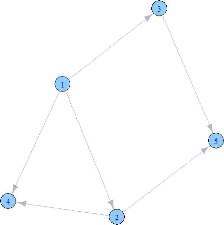
An example of Bayesian network
When bi-velocity discrete PSO works in BN structures learning, the position of each particle i is represented as
while the velocity is encoded as
where
4.2 Initial solution construction
To generate initial solutions, we use a method analogous to the one used in [25]. Each initial solution is derived by first starting with an empty graph dose not having any edges, and then adding the absent edges one by one to the current graph if and only if the new graph is a directed acyclic graph and the score of the new graph is higher than that of the previous graph. This procedure repeats until the number of added edges reaches the predefined value. By using the method mentioned above, a certain number of initial solutions are generated.
4.3 Bi-velocity discrete PSO with mutation operator
4.3.1 Updating rules
To keep the concept of original PSO in a continuous search space, different updating rules have been proposed in bi-velocity discrete PSO, which are described in detail as follows:
Velocity = Position1 – Position2: Suppose that X1 = (x11, x12,⋯, x1D) is in Position1 and X2 = (x21, x22,⋯, x2D) is in Position2, Position1 is better than Position2, then X2 must be learn from X1. The jth dimension of Vi is calculated according to the difference between x1j and x2j, if x1j is b, but x2j is not (b is 0 or 1), which means that the jth dimension of X2 is different from that of X1, X2 learns from X1, so
For example, if X1 = (1, 1, 0, 0, 1, 0, 0, 0) and X2 = (1, 0, 1, 1, 0, 0, 0, 1), then,
Velocity = Coefficient × Velocity: This equation represents that the Velocity is multiplied by ω or c × r. Because each element of the Velocity is the possibility for the position being 0 or 1, so the element that is larger than 1 is set to 1.
For example, c × r = (1.2, 0.8, 0.3, 1.5, 0.5, 0.2, 1.3, 0.7),
Velocity = Veloctiy1 + Velocity2: Suppose that V1 is Veloctiy1 and V2 is Velocity2, Vi = V1 + V2, the jth dimension
For example,
In the continuous searching space, the new position of a particle is calculated by adding the updated velocity to the current position. However, the position and velocity may not be added directly in the discrete searching space. In order to solve the discrete problem, a new updating method has been proposed as Eq. (10) [31]
in which α is a random value in [0, 1].
4.3.2 Mutation operation
When PSO is implemented, each particle moves toward its past best position and the global best position found so far, the exploitation ability is enhanced. However, according to the velocity and particle position updating rules, the numbers of nonzero elements in results of pbesti – Xi and gbest – Xi decrease and even becomes equal to zero with the increasing iterations. In this case, if the current global best position is not the global optimum, the particles in the swarm may be trapped in the local optima. To prevent premature convergence and enhance the exploration capability, a mutation strategy is adopted to conduct mutation on each new particle. The mutation probability depends on the problem dimension, in other words, it is determined by the number of nodes in BN structures learning problem, because a BN structure is represented by an n × n connectivity matrix whose diagonal elements are all zeros, and the position of a particle is encoded as a binary string according to the connectivity matrix. Thus, we define the mutation probability p = 1/(n2 – n), where n is the number of nodes. The mutation operator of a particle Xi = (xi1, xi2,⋯, xiD) is defined as
in which, m = 1,⋯,n.
4.4 Procedure of the proposed algorithm for BN structures learning
Based on the description above, the pseudo-code of BVD-MPSO-BN is presented in Algorithm 1. It starts with the initial solutions generated by the method described in section 4.2. Each particle in the swarm is encoded as a binary string corresponding to a directed acyclic graph and evaluated using the k2 metric. During iteration, each particle updates its velocity and position according to the updating rules presented in subsection 4.3.1. To increase the probability of escaping from a local optimum, the mutation operator is conducted on each new particle. Because each solution should be a direct acyclic graph, the direct cycles are removed from the new particle if it is a invalid solution. In order to detect and remove the cycles, we first use the depth first search algorithm to detect all back edges, and then invert or delete them. After removing the cycles, the proposed algorithm is executed to improve the past best position of each particle and the global best position of the population. During the main loop of the algorithm, the velocities and the positions of the particles are iteratively updated until a stopping criterion is met.
| Learning Bayesian Networks Based on Bi-Velocity Discrete PSO with Mutation Operator (BVD-MPSO-BN) |
|---|
| Require: |
| Input: Databases |
| Ensure: |
| Output: Bayesian Network |
|
5 Experimental results
In this section, we use several networks to test the behaviour of BVD-MPSO-BN. These networks are available in the software GeNie [1] In addition, we compare the proposed algorithm with other algorithms on benchmark networks. The experiments have been executed in a personal computer with Pentium(R) Dual-Core CPU, 2.0 GB memory, and Windows 7, all the algorithms have been implemented in the Matlab language.
5.1 Databases and parameter settings of the algorithms
In our experiments, three benchmark networks are selected, namely Alarm, Asia and Credit networks. Alarm network developed for on-line monitoring of patients in intensive care unites [33] contains 37 nodes and 46 arcs; Asia network is useful in demonstrating basics concepts of Bayesian networks in diagnosis [34], it is a simple graphical model and has 8 nodes and 8 arcs; Credit network for assessing credit worthiness of an individual was developed by Gerardina Hernandez as a class homework at the University of Pittsburgh, it is available in the GeNie software and consists of 12 nodes and 12 arcs. The databases used in our experiments are sampled from these benchmark networks by probabilistic logic sampling. In Table 1, the databases, the original networks, the number of cases in each database, the number of nodes in each network, the number of arcs in each network and the k2 scores for the original networks are listed.
Databases used in experiments
| Database | Original network | Number of cases | Number of nodes | Number of arcs | Score |
|---|---|---|---|---|---|
| Alarm-500 | Alarm | 500 | 37 | 46 | -2542.9 |
| Alarm-1000 | Alarm | 1000 | 37 | 46 | -5044.1 |
| Alarm-2000 | Alarm | 2000 | 37 | 46 | -9739.4 |
| Alarm-3000 | Alarm | 3000 | 37 | 46 | -14512.9 |
| Alarm-4000 | Alarm | 4000 | 37 | 46 | -19160.6 |
| Alarm-5000 | Alarm | 5000 | 37 | 46 | -237S0.5 |
| Asia-500 | Asia | 500 | 8 | 8 | -555.S |
| Asia-1000 | Asia | 1000 | 8 | 8 | -1101.1 |
| Asia-3000 | Asia | 3000 | 8 | 8 | -3326.3 |
| Credit-500 | Credit | 500 | 12 | 12 | -2741.2 |
| Credit-1000 | Credit | 1000 | 12 | 12 | -5360.6 |
| Credit-3000 | Credit | 3000 | 12 | 12 | -15S22.3 |
We compare BVD-MPSO-BN with other algorithms. BNC-PSO: structure learning Bayesian networks by particle swarm optimization [26], when BNC-PSO is implemented, the population size is 50, inertia weight ω decreases linearly from 0.95 to 0.4, acceleration coefficient c1 decreases linearly from 0.82 to 0.5 and acceleration coefficient c2 increases linearly from 0.4 to 0.83. An artificial bee colony algorithm for learning Bayesian networks (ABC-B) [24] had the following parameters: weighted coefficients for the pheromone α = 1 and the heuristic information β = 1, pheromone evaporation coefficient ρ = 0.1, switching parameter for exploitation versus exploration q0 = 0.8, maximum number of solution stagnation limit = 0.3, population size is equal to 40. The parameters for BVD-MPSO-BN were chosen as: the population size is 50, inertia weight ω = 0.1, acceleration coefficients c1 = c2 = 1.1.
5.2 Metrics of the performance
To measure the performance of proposed algorithm, we evaluate the learned results in terms of the k2 score and the structural difference (i.e., the differences between the learned structure and the original network).
The detailed descriptions of the metrics are defined as below:
HKS: the highest k2 score resulting from all trials carried out.
LKS: the lowest k2 score resulting from all trials.
AKS: the average k2 score (including the mean and the standard deviation) resulting from all trials.
AEA: the average number of edges accidentally added over all trials, it contains the mean and the standard deviation.
AED: the average number of edges accidentally deleted over all trials, it contains the mean and the standard deviation.
AEI: the average number of edges accidentally inverted over all trials, it contains the mean and the standard deviation.
LSD: the largest structural difference resulting from all trials.
SSD: the smallest structural difference resulting from all trials.
ASD: the average structural difference (including the mean and the standard deviation) resulting from all trials.
AIt: the average number of iterations needed to find an optimal solution over all trials, it contains the mean and the standard deviation.
AET: the average execution time over all trials.
5.3 Experimental analysis
5.3.1 Learning BNs using bi-velocity discrete PSO with mutation operator
To study the performance of BVD-MPSO-BN algorithm for Bayesian networks learning, we use it to recover the structures from databases sampled from the given benchmark networks. k2 score and structural difference as the basic metrics of the performance are adopted to evaluate the learned networks. We test the BVD-MPSO-BN algorithm by using the Alarm network with the sample size n = 500, 1000, 2000, 3000, 4000, 5000, the Asia network with the sample size n = 500, 1000, 3000 and the Credit network with the sample size n = 500, 1000, 3000. Table 2 reports the experimental results in terms of k2 score, the number of iterations and the execution time. Table 3 shows the experimental results based on the structural difference between the learned network and the original network. Each statistic in Table 2 and Table 3 is the average and standard deviation values over ten independent runs of BVD-MPSO-BN algorithm. We mark the best values in bold.
The k2 score, number of iterations and running time of BVD-MPSO-BN on different networks
| Database | HKS | LKS | AKS | AIt | AET |
|---|---|---|---|---|---|
| Alarm-500 | -2527.9 | -2554.9 | -2536.6±10.1 | 275.6±71.7 | 210 |
| Alarm-1000 | -5032.2 | -5054.9 | -5038.4±7.1 | 157.8±34.5 | 108.3 |
| Alarm-2000 | -9721.8 | -9727.2 | -9723.1±1.8 | 201±34.4 | 187.8 |
| Alarm-3000 | -14510.2 | -14515.0 | -14511.3±1.5 | 182.1±57.7 | 192.3 |
| Alarm-4000 | -19149.9 | -19154.2 | -19151.2±1.2 | 213.2±37.7 | 248.9 |
| Alarm-5000 | -23769.1 | -23773.2 | -23770.9±1.9 | 208.2±43.2 | 243.8 |
| Asia-500 | -555.2 | -555.2 | -555.2±0.0 | 15.3±10.8 | 13 |
| Asia-1000 | -1100.8 | -1101.2 | -1100.8±0.2 | 13.4±10.8 | 11.8 |
| Asia-3000 | -3325.9 | -3326.3 | -3326.0±0.2 | 9.5±5.7 | 11.0 |
| Credit-500 | -2707.3 | -2716.5 | -2709.9±3.9 | 14.1±6.0 | 18 |
| Credit-1000 | -5333.9 | -5338.7 | -5335.9±2.2 | 14±9.6 | 19.2 |
| Credit-3000 | -15806.2 | -15808.2 | -15806.4±0.7 | 14.6±5.6 | 28.1 |
The structural difference of BVD-MPSO-BN on different networks
| Database | LSD | SSD | ASD | AEA | AED | AEI |
|---|---|---|---|---|---|---|
| Alarm-500 | 14 | 7 | 12.6±2.8 | 7.4±1.6(5) | 2.8±0.90) | 2.4±1.7(0) |
| Alarm-1000 | 14 | 6 | 8.5±2.5 | 4.6±1.4 (2) | 2.5±0.5 (2) | 1.4±1.2 (0) |
| Alarm-2000 | 9 | 4 | 6±1.4 | 2.6±0.7 (1) | 2±0 (2) | 1.4±1.1 (0) |
| Alarm-3000 | 9 | 2 | 5.9±1.9 | 3.2±1.1 (1) | 1±0(1) | 1.4±1.0 (0) |
| Alarm-4000 | 7 | 2 | 3.6±1.7 | 1.7±0.7 (1) | 1±0(1) | 0.9±1.1 (0) |
| Alarm-5000 | 5 | 3 | 4.5±0.7 | 2.3±0.5 (2) | 1±0(1) | 1±1.2 (0) |
| Asia-500 | 4 | 3 | 3.5±0.5 | 2.5±0.5(2) | 1±0(1) | 0±0 (0) |
| Asia-1000 | 4 | 1 | 1.9±0.9 | 0.1±0.3 (0) | 1.1±0.3 (1) | 0.7±0.5 (0) |
| Asia-3000 | 2 | 0 | 1.1±0.6 | 0±0 (0) | 0.9±0.3 (0) | o.2±o.4(o) |
| Credit-500 | 2 | 1 | 1.8±0.4 | 0±0 (0) | 1±0(1) | 0.8±0.4(0) |
| Credit-1000 | 2 | 1 | 1.6±0.5 | 0±0 (0) | 1±0(1) | 0.6±0.5 (0) |
| Credit-3000 | 2 | 1 | 1.1±0.3 | 0±0 (0) | 0±0 (0) | 1.1±0.3 (0) |
As shown in Table 2, the difference between HKS and LKS is small on databases Alarm-2000, Alarm-3000, Alarm-4000 and Alarm-5000, except for Alarm-500 and Alarm-1000, which do not have enough samples to correctly learn Alarm networks. The algorithm also returns the small standard deviation, which indicates that the BVD-MPSO-BN algorithm is stable for the network with enough samples. For Asia network, the differences between HKS and LKS are smaller than 0.6 on database Asia-1000 and 0.4 on database Asia-3000, the algorithm returns the same k2 score on database Asia-500. In addition, the difference between AKS and the score of the original network is smaller than 0.6, which means that the score of the Asia network obtained by BVD-MPSO-BN algorithm is very close to that of the original network. For Credit network, the proposed algorithm obtains small standard deviation value and the difference between HKS and LKS, which indicates that the BVD-MPSO-BN algorithm also performs well in Credit network.
From the view of the structural difference, as shown in Table 3, the average and standard values in terms of ASD, AEA, AED and AEI are relatively small on databases sampled from Alarm, Asia and Credit networks. For Alarm network, the values of SSD on databases Alarm-3000 and Alarm-4000 are equal to two, which means that only two times of legitimate operations needed to change the learned network to the original one at the best case. The standard deviation values of AED are equal to zeros on databases Alarm-2000, Alarm-3000, Alarm-4000 and Alarm-5000, which means that the proposed algorithm learns the Alarm network with one or two edges accidentally deleted over ten runs. The average structural difference on database Alarm-500 is larger than 12, which means that the algorithm has poor performance on small databases. For Asia and Credit networks, the average and standard deviation values of AEA approach to zeros, and they are equal to zeros on databases Asia-3000, Credit-500, Credit-1000 and Credit-3000, which means that there are no edges accidentally added when the proposed algorithm learns the Asia network with sample size 3000 and the Credit network with sample size 500, 1000 and 3000. In the best case, the values of AEI are equal to zeros on databases generated from the benchmark networks, that is, there is no accidentally inverted edges in the best case.
The results related to the Alarm, Asia and Credit networks demonstrate that the proposed algorithm is stable for the large networks and able to find structures very close to the original structures for small networks. The performance of the proposed algorithm improves with the increasing sample size.
5.3.2 Learning BNs using different algorithms
Next, we compare BVD-MPSO-BN algorithm with BNC-PSO and ABC-B algorithms. The experimental results are presented in Table 4, Table 5 and Table 6. Each entry is the average and standard deviation values over ten independent runs of the different algorithms. The performance of the algorithms is evaluated based on the accuracy in terms of AKS, AEA, AED, AEI and AIt. The best values for different metrics are marked in bold.
The experimental results of three algorithms on Alarm network
| Database | Algorithm | AKS | ASD | AEA | AED | AEI | AIt |
|---|---|---|---|---|---|---|---|
| Alarm-500 | BVD-MPSO-BN | -2536.6±10.1 | 12.6±2.8 | 7.4±1.6 | 2.8±0.9 | 2.4±1.7 | 276.5±71.7 |
| BNC-PSO | -2548.6±10.0 | 21±2.6 | 12±2.3 | 4±0.9 | 5±1.6 | 308.2±64.6 | |
| ABC-B | -2532.7±4.4 | 10.1±1.6 | 4.7±0.8 | 3.3±0.8 | 2.1±0.7 | 272±25.6 | |
| Alarm-1000 | BVD-MPSO-BN | -5038.4±7.1 | 8.5±2.5 | 4.6±1.4 | 2.5±0.5 | 1.4±1.3 | 157.8±34.5 |
| BNC-PSO | -5040.0±2.7 | 10.4±2.2 | 5.6±1.0 | 2.7±0.5 | 2.1±1.7 | 276±45.7 | |
| ABC-B | -5043.6±8.1 | 9.1±3.2 | 3.4±1.5 | 3.2±0.6 | 2.5±1.7 | 176.8±37.5 | |
| Alarm-3000 | BVD-MPSO-BN | -14511.3±1.5 | 5.6±1.9 | 3.2±1.1 | 1±0 | 1.4±1.0 | 182.1±57.7 |
| BNC-PSO | -14516.2±5.3 | 8.2±1.9 | 4.5±1.1 | 1±0 | 2.7±1.1 | 272±55.3 | |
| ABC-B | -14516.5±7.5 | 6.0±1.9 | 2.0±0.9 | 1±0 | 3.0±1.3 | 162.4±49.6 | |
| Alarm-5000 | BVD-MPSO-BN | -23770.9±1.9 | 4.5±0.7 | 2.3±0.5 | 1±0 | 1.2±0.6 | 208.4±43.2 |
| BNC-PSO | -23770.9±6.5 | 4.5±2.6 | 2.3±1.2 | 1±0 | 1.2±1.7 | 208.4±59.4 | |
| ABC-B | -23771.2±5.3 | 3.7±2.5 | 2.0±1.4 | 1±0 | 1.3±1.6 | 153.9±42.7 |
The experimental results of three algorithms on Asia network
| Database | Algorithm | AKS | ASD | AEA | AED | AEI | AIt |
|---|---|---|---|---|---|---|---|
| Asia-500 | BVD-MPSO-BN | -555.2±0.0 | 3.5±0.5 | 2.5±0.5 | 1±0 | 0±0 | 15.3±10.7 |
| BNC-PSO | -555.2±0.0 | 3.3±0.5 | 2.3±0.5 | 1±0 | 0±0 | 18.1±6.6 | |
| ABC-B | -555.3±0.5 | 3.1±0.5 | 1.3±0.5 | 1±0 | 0.8±0.4 | 8.7±2.6 | |
| Asia-1000 | BVD-MPSO-BN | -1100.8±0.2 | 1.9±0.8 | 0.1±0.3 | 1.1±0.3 | 0.7±0.5 | 13.4±10.9 |
| BNC-PSO | -1100.8±0.2 | 1.9±0.8 | 0.1±0.3 | 1.1±0.3 | 0.7±0.5 | 17.3±11.4 | |
| ABC-B | -1100.9±0.3 | 1.4±0.8 | 0.2±0.4 | 1.2±0.4 | 0±0 | 24.1±19.5 | |
| Asia-3000 | BVD-MPSO-BN | -3325.9±0.1 | 1.1±0.5 | 0±0 | 0.9±0.3 | 0.2±0.4 | 9.5±5.7 |
| BNC-PSO | -3325.9±0 | 1.2±0.4 | 0±0 | 1±0 | 0.2±0.4 | 13.5±9.9 | |
| ABC-B | -3326.0±0.5 | 1.3±0.9 | 0.2±0.6 | 1.1±0.3 | 0±0 | 25.7±13.6 |
The experimental results of three algorithms on Credit network
| Database | Algorithm | AKS | ASD | AEA | AED | AEI | AIt |
|---|---|---|---|---|---|---|---|
| Credit-500 | BVD-MPSO-BN | -2709.9±3.9 | 1.8±0.4 | 0±0 | 1±0 | 0.8±0.4 | 14.1±6.0 |
| BNC-PSO | -2708.2±2.7 | 1.9±0.3 | 0±0 | 1±0 | 0.9±0.3 | 17.4±6.0 | |
| ABC-B | -2705.32±0 | 3±0 | 0±0 | 1±0 | 2±0 | 14.6±1.3 | |
| Credit-1000 | BVD-MPSO-BN | -5335.9±2.2 | 1.6±0.5 | 0±0 | 1±0 | 0.6±0.5 | 14.0±9.6 |
| BNC-PSO | -5335.8±2.1 | 2.0±0.7 | 0±0 | 1±0 | 1±0.7 | 23.5±16.4 | |
| ABC-B | -5354.9±10.7 | 2.0±0.6 | 0.1±0.3 | 1.9±0.6 | 0±0 | 25.9±10.1 | |
| Credit-3000 | BVD-MPSO-BN | -15806.4±0.7 | 1.1±0.3 | 0±0 | 0±0 | 1.1±0.3 | 14.6±5.6 |
| BNC-PSO | -15813.0±5.7 | 1.1±0.7 | 0±0 | 0.5±0.5 | 0.6±0.7 | 26.0±11.0 | |
| ABC-B | -15815.7±0 | 1.0±0 | 0±0 | 1±0 | 0±0 | 14.6±3.2 |
Table 4 shows the experimental results of three different algorithms on databases sampled from Alarm network. From the perspective of k2 score, BVD-MPSO-BN achieves the best values of AKS on databases Alarm-3000 and Alarm-5000. Although, BVD-MPSO-BN obtains the higher k2 score on databases Alarm-1000 compared with BNC-PSO, the standard deviation is larger than that obtained by BNC-PSO. ABC-B algorithm returns the best k2 score on small database Alarm-500. From the view of structural difference, the ASD values of BVD-MPSO-BN on databases Alarm-1000 and Alarm-3000 are the smallest among those of three algorithms. The ASD values returned by ABC-B algorithm on databases Alarm-500 and Alarm-5000 are smaller than that returned by other algorithms. Although ABC-B achieves the smallest average value of ASD on database Alarm-5000, the standard deviation is larger than that of BVD-MPSO-BN. It is obvious that BNC-PSO obtains networks with more incorrect edges compared with original networks on database Alarm-500. The values of AEA returned by ABC-B on different databases sample from Alarm network are the best among those of three algorithms. BVD-MPSO-BN achieves the smallest values of AED on database Alarm-500 and Alarm-1000, the AED values of BNC-PSO and ABC-B on databases Alarm-3000 and Alarm-5000 are the same as that of BVD-MPSO-BN, and they are equal to ones, which means that each of three algorithms learns the BN structures with one edge accidentally deleted on each trial carried out. BVD-MPSO-BN obtains the best values of AEI on databases Alarm-1000, Alarm-500 and Alarm-5000. From the view of the number of iterations, ABC-B often needs less number of iterations compared with BVD-MPSO-BN on databases Alarm-500, Alarm-3000 and Alarm-5000.
From the experimental results on Asia network with sample size n = 500, 1000, 3000 in Table 5, we observe that the BVD-MPSO-BN and BNC-PSO algorithms achieve the same well k2 score and structural difference on databases Asia-500 and Asia-1000, they learn the BNs from database Asia-3000 with no edges accidentally added over ten executions. In comparison to the use of ABC-B algorithm, BVD-MPSO-BN algorithm can obtain higher k2 score, while the ASD values returned by ABC-B algorithm on databases Asia-500 and Asia-1000 are the smallest among three algorithms. There is no accidentally inverted edges generated by BVD-MPSO-BN and BNC-PSO algorithms on database Asia-500. However, the average number of iterations of BVD-MPSO-BN algorithm is the smallest among three algorithms on databases Asia-1000 and Asia-3000.
The experimental results of three algorithms on the Credit network are presented in Table 6. For k2 score, BVD-MPSO-BN algorithm does not perform well on databases Credit-500 and Credit-1000, but still obtains relatively good result on databases Credit-3000. From the view of the structure difference, we observe that BVD-MPSO-BN obtains the best ASD results on databases Credit-500 and Credit-1000. BVD-MPSO-BN and BNC-PSO get the same AEA results and BVD-MPSO-BN obtains the best AED results on three databases. ABC-B obtains the best AEI results on databases Credit-1000 and Credit-5000, and BVD-MPSO-BN obtains the best AEI result on database Credit-500. The average number of iteration of BVD-MPSO-BN is smaller or at least not larger than that of the other two algorithms.
To test the time performance of the proposed algorithm, we evaluate three algorithms on Alarm network with sample size n = 1000, 3000, 5000, Asia network with sample size n = 1000, 3000 and Credit network with sample size n = 1000, 3000. Fig.(2) shows the average running time of three algorithms on different networks. It is obvious that the searching time of the proposed algorithm is the smallest among three algorithms. For BNC-PSO algorithm, the reason is that BVD-MPSO-BN keeps the advantage of fast convergence of classical PSO, while BNC-PSO was proposed by combining PSO with Genetic Algorithm. For ABC-B algorithm, during each iteration, each employed bee finds a new solution in its neighborhood by testing and comparing the k2 scores of four operators (addition, deletion, reversion and move). In addition, each onlooker determines a new solution by performing two knowledge-guided operators or four simple operators and comparing their k2 scores, so it is time consuming to compute the k2 score. Although the number of iterations of ABC-B is often less than that of BVD-MPSO-BN, ABC-B takes much time to reach the near-optimal solutions. Meanwhile, we analyze the changing of time requirement as the changing of sample size. Fig.(3) shows the average results of BVD-MPSO-BN in comparison to ABC-B and BNC-PSO algorithms on databases sampled from Alarm network. Three algorithms generally take much time on learning BNs from large databases. It is obvious that the execution time of the proposed algorithm increases slowly with the increase of the sample size, whereas ABC-B and BNC-PSO algorithms are sensitive to the sample capacity. The overall results demonstrate that BVD-MPSO-BN algorithm is superior to ABC-B and BNC-PSO algorithms in terms of execution time.
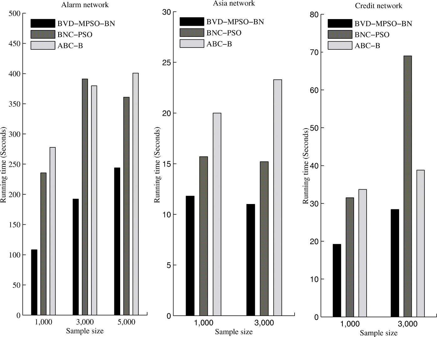
Time performance on three different networks.
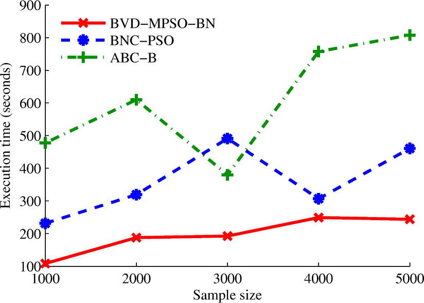
Time performance of three algorithms on Alarm network.
Fig. 4 shows the convergence characteristics of three heuristic algorithms on database Alarm-5000. It is obvious that the final solutions of three algorithms are close to each other. However, the proposed algorithm converges to the optimal solutions faster than both BNC-PSO and ABC-B algorithms. BNC-PSO performs better than ABC-B at the beginning because particles in PSO learn from better and best solutions so that the population quickly converges to the optimal solution. Once the particles are close to the best solution, the convergence speed becomes slower. However, with the help of mutation operator, the particles in proposed algorithm are easy to jump out of the likely local optima, and hence the fast convergence speed could be remained through the whole evolutionary progress.
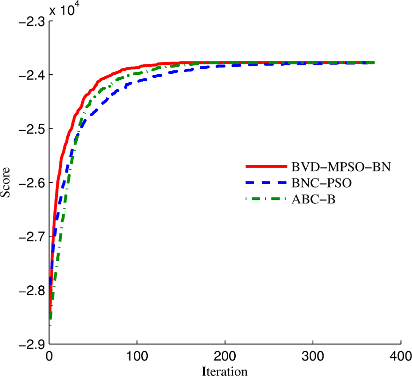
The score convergence of three algorithms on Alarm-5000.
Based on the observations above, we conclude that BVD-MPSO-BN can guarantee to learn good-quality networks. BVD-MPSO-BN not only keeps the powerful searching capability in finding the optimal solution, but also prevents the particles in swarm from trapping in the local optima.
6 Conclusion
In this paper, we propose a novel score-based algorithm for BNs learning. PSO is a swarm intelligence globalized search algorithm with the advantages of simple computation and rapid convergence capability. However, with the increasing of the number of iterations, the quality of the solution can not be improved, and the algorithm converges to the local optima. In other words, it is easy for PSO to suffer from the premature convergence. To overcome the drawback of the PSO and learn BN structures from data, bi-velocity discrete PSO with mutation algorithm has been proposed. We make a proper balance between exploration and exploitation ability of the proposed algorithm. The experimental results on the databases generated from the benchmark networks demonstrate the effectiveness of our method. Comparing with the BNC-PSO algorithm for BNs learning, the advantage of our algorithm not only lies in its less computation time but also lies in its less error rate between the learned structure and the original network. In the comparison to the use of the ABC-B algorithm, when the number of samples available for structure learning is large, the proposed algorithm performs well and has the better average accurate. The experimental results illustrate the superiority of the proposed algorithm in learning BNs from the data. In this paper, the databases are completely observed, however, there may exist missing data or data with hidden variables in practice. Extending swarm-based algorithms to learn BN structures with incomplete data is our future work. In addition, the performance of the proposed algorithm decreases with the decreasing sample size. Thus, future work will consider the method for structure learning on small databases.
Acknowledgement
The research is supported by the National Natural Science Foundation of China (Grant No.61373174) and (Grant No.11401454).
References
[1] Jayech K., Mahjoub M.A., Ghanmi N., Application of bayesian networks for pattern recognition: Character recognition case, Proceedings of 6th International Conference on Sciences of Electronics, Technologies of Information and Telecommunications (SETIT), 2012, IEEE, pp. 748–75710.1109/SETIT.2012.6482008Search in Google Scholar
[2] Wang Q., Gao X., Chen D., Pattern recognition for ship based on bayesian networks, Proceedings of Fourth International Conference on Fuzzy Systems and Knowledge Discovery, 2007, vol. 4, IEEE, pp. 684–68810.1109/FSKD.2007.447Search in Google Scholar
[3] Nikovski D., Constructing bayesian networks for medical diagnosis from incomplete and partially correct statistics, IEEE Transactions on Knowledge and Data Engineering, 2000, 12(4), 509–51610.1109/69.868904Search in Google Scholar
[4] AlObaidi A.T.S., Mahmood N.T., Modified full bayesian networks classifiers for medical diagnosis, Proceedings of International Conference on Advanced Computer Science Applications and Technologies (ACSAT), 2013, IEEE, pp. 5–1210.1109/ACSAT.2013.10Search in Google Scholar
[5] Bonafede C.E., Giudici P., Bayesian networks for enterprise risk assessment, Physica A: Statistical Mechanics and its Applications, 2007, 382(1), 22–2810.1016/j.physa.2007.02.065Search in Google Scholar
[6] Liu Q., Pérès F., Tchangani A., Object oriented bayesian network for complex system risk assessment, IFAC-PapersOnLine, 2016, 49(28), 31–3610.1016/j.ifacol.2016.11.006Search in Google Scholar
[7] Li Y., Ngom A., The max-min high-order dynamic bayesian network learning for identifying gene regulatory networks from time-series microarray data, IEEE Symposium on Computational Intelligence in Bioinformatics and Computational Biology (CIBCB), 2013, IEEE, pp. 83–9010.1109/CIBCB.2013.6595392Search in Google Scholar
[8] Tamada Y., Imoto S., Araki H., Nagasaki M., Print C., Charnock-Jones D.S., Miyano S., Estimating genome-wide gene networks using nonparametric bayesian network models on massively parallel computers, IEEE/ACM Transactions on Computational Biology and Bioinformatics, 2011, 8(3), 683–69710.1109/TCBB.2010.68Search in Google Scholar PubMed
[9] Wang M., Chen Z., Cloutier S., A hybrid bayesian network learning method for constructing gene networks, Computational Biology and Chemistry, 2007, 31(5-6), 361–37210.1016/j.compbiolchem.2007.08.005Search in Google Scholar PubMed
[10] Margaritis D., Learning bayesian network model structure from data(phd thesis), Tech. rep., Carnegie-Mellon Univ Pittsburgh PA School of Computer Science, 2003Search in Google Scholar
[11] Tsamardinos I., Aliferis C.F., Statnikov A.R., Statnikov E., Algorithms for large scale markov blanket discovery, Proceedings of FLAIRS Conference, 2003, vol. 2, pp. 376–380Search in Google Scholar
[12] Tsamardinos I., Aliferis C.F., Statnikov A., Time and sample efficient discovery of markov blankets and direct causal relations, Proceedings of Ninth ACM SIGKDD International Conference on Knowledge Discovery and Data Mining, 2003, ACM, pp. 673–67810.1145/956750.956838Search in Google Scholar
[13] Pena J.M., Nilsson R., Björkegren J., Tegnér J., Towards scalable and data efficient learning of markov boundaries, International Journal of Approximate Reasoning, 2007, 45(2), 211–23210.1016/j.ijar.2006.06.008Search in Google Scholar
[14] Cooper G.F., Herskovits E., A bayesian method for the induction of probabilistic networks from data, Machine learning, 1992, 9(4), 309–34710.1007/BF00994110Search in Google Scholar
[15] Alcobé J.R., Incremental hill-climbing search applied to bayesian network structure learning, Proceedings of 15th European Conference on Machine Learning, 2004, IEEE Pisa, Italy, pp. 1–10Search in Google Scholar
[16] Chickering D.M., Optimal structure identification with greedy search, Journal of Machine Learning Research, 2002, 3(11), 507–554Search in Google Scholar
[17] Chickering D.M., Geiger D., Heckerman D., et al., Learning bayesian networks is np-hard, Tech. rep., Citeseer, 1994Search in Google Scholar
[18] Tonda A.P., Lutton E., Reuillon R., Squillero G., Wuillemin P.H., Bayesian network structure learning from limited datasets through graph evolution, Proceedings of European Conference on Genetic Programming, 2012, pp. 254–26510.1007/978-3-642-29139-5_22Search in Google Scholar
[19] Tonda A., Lutton E., Squillero G., Wuillemin P.H., A memetic approach to bayesian network structure learning, Lecture Notes in Computer Science, 2013, 7835, 102–11110.1007/978-3-642-37192-9_11Search in Google Scholar
[20] Ji J., Yang C., Liu J., Liu J., Yin B., A comparative study on swarm intelligence for structure learning of bayesian networks, Soft Computing, 2017, 21(22), 6713–673810.1007/s00500-016-2223-xSearch in Google Scholar
[21] De Campos L.M., Fernandez-Luna J.M., Gámez J.A., Puerta J.M., Ant colony optimization for learning bayesian networks, International Journal of Approximate Reasoning, 2002, 31(3), 291–31110.1016/S0888-613X(02)00091-9Search in Google Scholar
[22] Daly R., Shen Q., et al., Learning bayesian network equivalence classes with ant colony optimization, Journal of Artificial Intelligence Research, 2009, 35(1), 391–44710.1613/jair.2681Search in Google Scholar
[23] Jun-Zhong J., Zhang H.X., Ren-Bing H., Chun-Nian L., A bayesian network learning algorithm based on independence test and ant colony optimization, Acta Automatica Sinica, 2009, 35(3), 281–28810.3724/SP.J.1004.2009.00281Search in Google Scholar
[24] Ji J., Wei H., Liu C., An artificial bee colony algorithm for learning bayesian networks, Soft Computing, 2013, 17(6), 983–99410.1007/s00500-012-0966-6Search in Google Scholar
[25] Yang C., Ji J., Liu J., Liu J., Yin B., Structural learning of bayesian networks by bacterial foraging optimization, International Journal of Approximate Reasoning, 2016, 69, 147–16710.1016/j.ijar.2015.11.003Search in Google Scholar
[26] Gheisari S., Meybodi M.R., Bnc-pso: structure learning of bayesian networks by particle swarm optimization, Information Sciences, 2016, 348, 272–28910.1016/j.ins.2016.01.090Search in Google Scholar
[27] Wang T., Yang J., A heuristic method for learning bayesian networks using discrete particle swarm optimization, Knowledge and Information Systems, 2010, 24(2), 269–28110.1007/s10115-009-0239-6Search in Google Scholar
[28] Xing-Chen H., Zheng Q., Lei T., Li-Ping S., Learning bayesian network structures with discrete particle swarm optimization algorithm, IEEE Symposium on Foundations of Computational Intelligence, 2007, IEEE, pp. 47–5210.1109/FOCI.2007.372146Search in Google Scholar
[29] Aouay S., Jamoussi S., Ayed Y.B., Particle swarm optimization based method for bayesian network structure learning, Proceedings of 5th International Conference on Modeling, Simulation and Applied Optimization (ICMSAO), 2013, IEEE, pp. 1–610.1109/ICMSAO.2013.6552569Search in Google Scholar
[30] Zhong W.L., Huang J., Zhang J., A novel particle swarm optimization for the steiner tree problem in graphs, IEEE Congress on Evolutionary Computation (IEEE World Congress on Computational Intelligence), 2008, IEEE, pp. 2460–2467Search in Google Scholar
[31] Shen M., Zhan Z.H., Chen W.N., Gong Y.J., Zhang J., Li Y., Bi-velocity discrete particle swarm optimization and its application to multicast routing problem in communication networks, IEEE Transactions on Industrial Electronics, 2014, 61(12), 7141–715110.1109/TIE.2014.2314075Search in Google Scholar
[32] Larrañaga P., Poza M., Yurramendi Y., Murga R.H., Kuijpers C.M.H., Structure learning of bayesian networks by genetic algorithms: A performance analysis of control parameters, IEEE Transactions on Ppattern Analysis and Machine Intelligence, 1996, 18(9), 912–92610.1109/34.537345Search in Google Scholar
[33] Beinlich I.A., Suermondt H.J., Chavez R.M., Cooper G.F., The alarm monitoring system: A case study with two probabilistic inference techniques for belief networks, AIME 89, Springer, 1989, pp. 247–25610.1007/978-3-642-93437-7_28Search in Google Scholar
[34] Lauritzen S.L., Spiegelhalter D.J., Local computations with probabilities on graphical structures and their application to expert systems, Journal of the Royal Statistical Society. Series B (Methodological), 1988, 157–22410.1111/j.2517-6161.1988.tb01721.xSearch in Google Scholar
© 2018 Wang and Liu, published by De Gruyter
This work is licensed under the Creative Commons Attribution-NonCommercial-NoDerivatives 4.0 License.
Articles in the same Issue
- Regular Articles
- Algebraic proofs for shallow water bi–Hamiltonian systems for three cocycle of the semi-direct product of Kac–Moody and Virasoro Lie algebras
- On a viscous two-fluid channel flow including evaporation
- Generation of pseudo-random numbers with the use of inverse chaotic transformation
- Singular Cauchy problem for the general Euler-Poisson-Darboux equation
- Ternary and n-ary f-distributive structures
- On the fine Simpson moduli spaces of 1-dimensional sheaves supported on plane quartics
- Evaluation of integrals with hypergeometric and logarithmic functions
- Bounded solutions of self-adjoint second order linear difference equations with periodic coeffients
- Oscillation of first order linear differential equations with several non-monotone delays
- Existence and regularity of mild solutions in some interpolation spaces for functional partial differential equations with nonlocal initial conditions
- The log-concavity of the q-derangement numbers of type B
- Generalized state maps and states on pseudo equality algebras
- Monotone subsequence via ultrapower
- Note on group irregularity strength of disconnected graphs
- On the security of the Courtois-Finiasz-Sendrier signature
- A further study on ordered regular equivalence relations in ordered semihypergroups
- On the structure vector field of a real hypersurface in complex quadric
- Rank relations between a {0, 1}-matrix and its complement
- Lie n superderivations and generalized Lie n superderivations of superalgebras
- Time parallelization scheme with an adaptive time step size for solving stiff initial value problems
- Stability problems and numerical integration on the Lie group SO(3) × R3 × R3
- On some fixed point results for (s, p, α)-contractive mappings in b-metric-like spaces and applications to integral equations
- On algebraic characterization of SSC of the Jahangir’s graph 𝓙n,m
- A greedy algorithm for interval greedoids
- On nonlinear evolution equation of second order in Banach spaces
- A primal-dual approach of weak vector equilibrium problems
- On new strong versions of Browder type theorems
- A Geršgorin-type eigenvalue localization set with n parameters for stochastic matrices
- Restriction conditions on PL(7, 2) codes (3 ≤ |𝓖i| ≤ 7)
- Singular integrals with variable kernel and fractional differentiation in homogeneous Morrey-Herz-type Hardy spaces with variable exponents
- Introduction to disoriented knot theory
- Restricted triangulation on circulant graphs
- Boundedness control sets for linear systems on Lie groups
- Chen’s inequalities for submanifolds in (κ, μ)-contact space form with a semi-symmetric metric connection
- Disjointed sum of products by a novel technique of orthogonalizing ORing
- A parametric linearizing approach for quadratically inequality constrained quadratic programs
- Generalizations of Steffensen’s inequality via the extension of Montgomery identity
- Vector fields satisfying the barycenter property
- On the freeness of hypersurface arrangements consisting of hyperplanes and spheres
- Biderivations of the higher rank Witt algebra without anti-symmetric condition
- Some remarks on spectra of nuclear operators
- Recursive interpolating sequences
- Involutory biquandles and singular knots and links
- Constacyclic codes over 𝔽pm[u1, u2,⋯,uk]/〈 ui2 = ui, uiuj = ujui〉
- Topological entropy for positively weak measure expansive shadowable maps
- Oscillation and non-oscillation of half-linear differential equations with coeffcients determined by functions having mean values
- On 𝓠-regular semigroups
- One kind power mean of the hybrid Gauss sums
- A reduced space branch and bound algorithm for a class of sum of ratios problems
- Some recurrence formulas for the Hermite polynomials and their squares
- A relaxed block splitting preconditioner for complex symmetric indefinite linear systems
- On f - prime radical in ordered semigroups
- Positive solutions of semipositone singular fractional differential systems with a parameter and integral boundary conditions
- Disjoint hypercyclicity equals disjoint supercyclicity for families of Taylor-type operators
- A stochastic differential game of low carbon technology sharing in collaborative innovation system of superior enterprises and inferior enterprises under uncertain environment
- Dynamic behavior analysis of a prey-predator model with ratio-dependent Monod-Haldane functional response
- The points and diameters of quantales
- Directed colimits of some flatness properties and purity of epimorphisms in S-posets
- Super (a, d)-H-antimagic labeling of subdivided graphs
- On the power sum problem of Lucas polynomials and its divisible property
- Existence of solutions for a shear thickening fluid-particle system with non-Newtonian potential
- On generalized P-reducible Finsler manifolds
- On Banach and Kuratowski Theorem, K-Lusin sets and strong sequences
- On the boundedness of square function generated by the Bessel differential operator in weighted Lebesque Lp,α spaces
- On the different kinds of separability of the space of Borel functions
- Curves in the Lorentz-Minkowski plane: elasticae, catenaries and grim-reapers
- Functional analysis method for the M/G/1 queueing model with single working vacation
- Existence of asymptotically periodic solutions for semilinear evolution equations with nonlocal initial conditions
- The existence of solutions to certain type of nonlinear difference-differential equations
- Domination in 4-regular Knödel graphs
- Stepanov-like pseudo almost periodic functions on time scales and applications to dynamic equations with delay
- Algebras of right ample semigroups
- Random attractors for stochastic retarded reaction-diffusion equations with multiplicative white noise on unbounded domains
- Nontrivial periodic solutions to delay difference equations via Morse theory
- A note on the three-way generalization of the Jordan canonical form
- On some varieties of ai-semirings satisfying xp+1 ≈ x
- Abstract-valued Orlicz spaces of range-varying type
- On the recursive properties of one kind hybrid power mean involving two-term exponential sums and Gauss sums
- Arithmetic of generalized Dedekind sums and their modularity
- Multipreconditioned GMRES for simulating stochastic automata networks
- Regularization and error estimates for an inverse heat problem under the conformable derivative
- Transitivity of the εm-relation on (m-idempotent) hyperrings
- Learning Bayesian networks based on bi-velocity discrete particle swarm optimization with mutation operator
- Simultaneous prediction in the generalized linear model
- Two asymptotic expansions for gamma function developed by Windschitl’s formula
- State maps on semihoops
- 𝓜𝓝-convergence and lim-inf𝓜-convergence in partially ordered sets
- Stability and convergence of a local discontinuous Galerkin finite element method for the general Lax equation
- New topology in residuated lattices
- Optimality and duality in set-valued optimization utilizing limit sets
- An improved Schwarz Lemma at the boundary
- Initial layer problem of the Boussinesq system for Rayleigh-Bénard convection with infinite Prandtl number limit
- Toeplitz matrices whose elements are coefficients of Bazilevič functions
- Epi-mild normality
- Nonlinear elastic beam problems with the parameter near resonance
- Orlicz difference bodies
- The Picard group of Brauer-Severi varieties
- Galoisian and qualitative approaches to linear Polyanin-Zaitsev vector fields
- Weak group inverse
- Infinite growth of solutions of second order complex differential equation
- Semi-Hurewicz-Type properties in ditopological texture spaces
- Chaos and bifurcation in the controlled chaotic system
- Translatability and translatable semigroups
- Sharp bounds for partition dimension of generalized Möbius ladders
- Uniqueness theorems for L-functions in the extended Selberg class
- An effective algorithm for globally solving quadratic programs using parametric linearization technique
- Bounds of Strong EMT Strength for certain Subdivision of Star and Bistar
- On categorical aspects of S -quantales
- On the algebraicity of coefficients of half-integral weight mock modular forms
- Dunkl analogue of Szász-mirakjan operators of blending type
- Majorization, “useful” Csiszár divergence and “useful” Zipf-Mandelbrot law
- Global stability of a distributed delayed viral model with general incidence rate
- Analyzing a generalized pest-natural enemy model with nonlinear impulsive control
- Boundary value problems of a discrete generalized beam equation via variational methods
- Common fixed point theorem of six self-mappings in Menger spaces using (CLRST) property
- Periodic and subharmonic solutions for a 2nth-order p-Laplacian difference equation containing both advances and retardations
- Spectrum of free-form Sudoku graphs
- Regularity of fuzzy convergence spaces
- The well-posedness of solution to a compressible non-Newtonian fluid with self-gravitational potential
- On further refinements for Young inequalities
- Pretty good state transfer on 1-sum of star graphs
- On a conjecture about generalized Q-recurrence
- Univariate approximating schemes and their non-tensor product generalization
- Multi-term fractional differential equations with nonlocal boundary conditions
- Homoclinic and heteroclinic solutions to a hepatitis C evolution model
- Regularity of one-sided multilinear fractional maximal functions
- Galois connections between sets of paths and closure operators in simple graphs
- KGSA: A Gravitational Search Algorithm for Multimodal Optimization based on K-Means Niching Technique and a Novel Elitism Strategy
- θ-type Calderón-Zygmund Operators and Commutators in Variable Exponents Herz space
- An integral that counts the zeros of a function
- On rough sets induced by fuzzy relations approach in semigroups
- Computational uncertainty quantification for random non-autonomous second order linear differential equations via adapted gPC: a comparative case study with random Fröbenius method and Monte Carlo simulation
- The fourth order strongly noncanonical operators
- Topical Issue on Cyber-security Mathematics
- Review of Cryptographic Schemes applied to Remote Electronic Voting systems: remaining challenges and the upcoming post-quantum paradigm
- Linearity in decimation-based generators: an improved cryptanalysis on the shrinking generator
- On dynamic network security: A random decentering algorithm on graphs