A Geršgorin-type eigenvalue localization set with n parameters for stochastic matrices

Theorem 1.1

([8, Theorem 3.4]). LetA = [a_ij] ∈ ℝ^n×nbe a stochastic matrix. If λ ∈ σ(A)∖{1}, then

whereγ(A) = maxi∈N (a_ii − l_i(A)), l_i(A) = minj≠ia_jiand trace(A) is the trace ofA.

Theorem 1.2

([15, Theorem 6]). LetA = [a_ij] ∈ ℝ^n×nbe a stochastic matrix. If λ ∈ σ(A)∖{1}, then

whereγ̃(A) = maxi∈N (L_i(A) − a_ii) andL_i(A) = maxj≠ia_ji.

Theorem 1.3

([11, 12]). LetA = [a_ij] ∈ ℝ^n×nbe a stochastic matrix. If λ ∈ σ(A)∖{1}, then

and

where

andCq_i(A) = ∑j≠i |a_ji − q_i(A)|.

Theorem 1.4

([11, Theorems 3.3 and 3.8]). LetA = [a_ij] ∈ ℝ^n×nbe a stochastic matrix. If λ ∈ σ(A)∖{1}, then

and

where

and

Lemma 2.1

([8, 11, 12]). LetA = [a_ij] ∈ ℝ^n×nbe a stochastic matrix. For anyd = [d₁,d₂, …, d_n]^T ∈ ℝⁿ, ifμ ∈ σ(A)∖{1}, then − μis an eigenvalue of the matrix

Theorem 2.2

LetA = [a_ij] ∈ ℝ^n×nbe a stochastic matrix. If λ ∈ σ(A)∖{1}, then for anyα_i ∈ [0, 1], i ∈ N,

where

and

Proof

Let Bαi=edT−A=[bijαi], whered=Lαi(A)=[L1α1(A),L2α2(A),…,Lnαn(A)]T. By applying the Geršgorin circle theorem to B^α_i, we have that for any λ̂ ∈ σ (B^α_i),

By Lemma 2.1, we have for λ ∈ σ(A)∖{1}, then −λ ∈ σ(B^α_i), that is,

Furthermore, note that for any i ∈ N,

and

Hence,

where ΓistoLαi(A) = {z ∈ ℂ : |α_iL_i(A) + (1 − α_i)l_i(A) − a_ii + z| ≤ CLiαi(A)}. □

Example 2.3

Consider the first 50 stochastic matrices generated by the MATLAB code

and takeα_i ∈ [0, 1] fori = 1, 2, …, 10 by the MATLAB code

By drawing the setsΓ^stoLα(A) inTheorem 2.2and

inTheorems 1.1and1.2, it is not difficult to see that the number ofΓ^stoLα(A) ⊂ Γis 46, that if 1 ∉ Γ, then 1 ∉ Γ^stoLα(A), and that if 1 ∈ Γ, thenΓ^stoLα(A) may not contain the trivial eigenvalue 1 (also see Table 1). So, by these examples, we conclude that the set inTheorem 2.2captures all eigenvalues different from 1 of a stochastic matrix more precisely than the sets inTheorem 1.1andTheorem 1.2in some cases.

Remark 2.4

1. Whenα_i = 1 for eachi ∈ N, thenLiαi(A) = L_i(A) andCLiαi(A) = CL_i(A) for anyi ∈ N, which impliesΓ^stoLα(A) reduces toΓ^stoL(A) inTheorem 1.4;

2. Whenαi=Vi(A)−li(A)Li(A)−li(A) ∈ [0, 1] andL_i(A) > l_i(A) for eachi ∈ N, thenLiαi(A) = V_i(A) andCLiαi(A) = CV_i(A) for anyi ∈ N. On the other hand, if for somei ∈ N, L_i(A) = l_i(A), then for anyα_i ∈ [0, 1] we also haveLiαi(A) = V_i(A) andCLiαi(A) = CV_i(A). These implyΓ^stoLα(A) reduces toΓ^stoV(A) inTheorem 1.4;

3. Whenαi=qi(A)−li(A)Li(A)−li(A) ∈ [0, 1] andL_i(A) > l_i(A) for eachi ∈ N, thenLiαi(A) = q_i(A) andCLiαi(A) = Cq_i(A) for anyi ∈ N. On the other hand, if for somei ∈ N, L_i(A) = l_i(A), then for anyα_i ∈ [0, 1] we also haveLiαi(A) = q_i(A) andCLiαi(A) = Cq_i(A). These implyΓ^stoLα(A) reduces toΓ^stoq(A) inTheorem 1.3;

4. Whenαi=vi(A)−li(A)Li(A)−li(A) ∈ [0, 1] andL_i(A) > l_i(A) for eachi ∈ N, thenLiαi(A) = v_i(A) andCLiαi(A) = Cv_i(A) for anyi ∈ N. On the other hand, if for somei ∈ N, L_i(A) = l_i(A), then for anyα_i ∈ [0, 1] we also haveLiαi(A) = v_i(A) andCLiαi(A) = Cv_i(A). These implyΓ^stoLα(A) reduces toΓ^stov(A) inTheorem 1.3;

5. Whenα_i = 0 for eachi ∈ N, thenLiαi(A) = l_i(A) andCLiαi(A) = Cl_i(A) for anyi ∈ N, which impliesΓ^stoLα(A) reduces toΓ^stol(A) in Theorem 1.3.

Remark 2.5

LetA = [a_ij] ∈ ℝ^n×nbe a stochastic matrix. If λ ∈ σ(A)∖{1}, then

Furthermore, Γ^[0,1] (A) ⊆ (Γ^stoL(A) ⋂ Γ^stoV(A) ⋂ Γ^stoq(A) ⋂ Γ^stov(A) ⋂ Γ^stol(A)).

The set Γ^[0,1] (A) in Remark 2.5 is not of much practical use because it involves some parameters α_i. In fact, we can take some special α_i in practice, which is illustrated by the following example.

Example 2.6

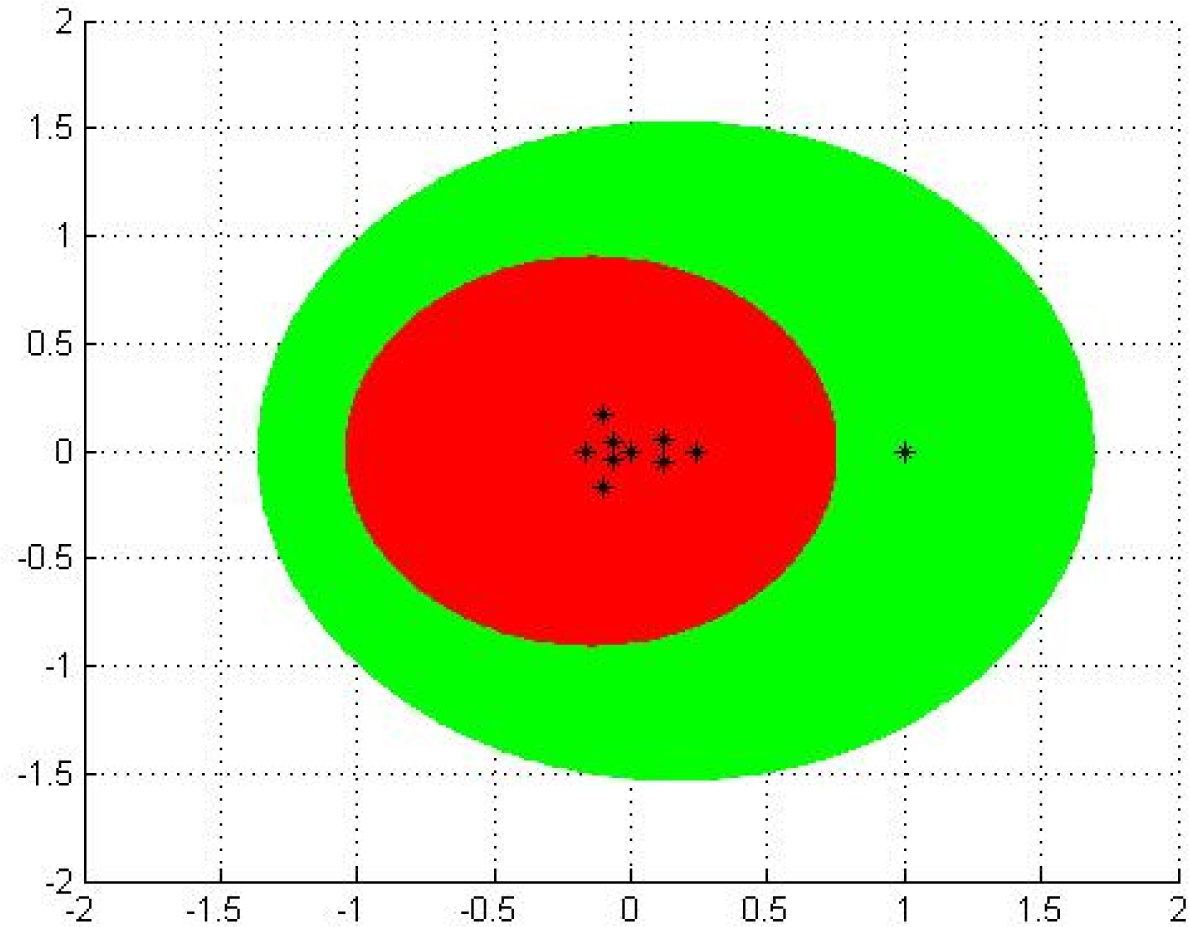
Consider the third stochastic matrixA in Example 2.3. ByTable 1, we have that

which is shown inFigure 1, whereΓ^stoLα(A) is drawn slightly thicker thanΓ. Furthermore, we take the first 3 vectors

Fig. 1

Γ^stoLα(A) ⊈ Γ, andΓ ⊈ Γ^stoLα(A)

generated by the MATLAB code alpha = rand(1, 10), that is,

and

ByRemark 2.5, we have that for any λ ∈ σ(A)∖{1},

We draw this set in the complex plane, seeFigure 2. It is easy to see

Fig. 2

(Γ^stoLα(1)(A) ⋂ Γ^stoLα(2)(A) ⋂ Γ^stoLα(3)(A)) ⊂ Γ

and

Proposition 2.7

LetA = [a_ij] ∈ ℝ^n×nbe a stochastic matrix. If for someᾱ_i ∈ [0, 1], i ∈ N,

whereCLiα¯iis defined as (2), thenAis nonsingular.

Proof

Suppose that A is singular, that is, 0 ∈ σ (A). From Theorem 2.2, we have that for any α_i ∈ [0, 1], i ∈ N,

In particular,

Hence, there is an index i₀ ∈ N such that

This contradicts (3). The conclusion follows.  □

Theorem 3.1

Let A = [a_ij] ∈ ℝ^{n × n}be a stochastic matrix. If λ ∈ σ(A)∖{1}, then

whereρ[0,1]=maxi∈Nminαi∈[0,1]∑j=1n|αiLi(A)+(1−αi)li(A)−aji|.

Proof

Let

where

Therefore, each f_i(α_i), i ∈ N is a continuous function of α_i ∈ [0,1], and there are α̃_i ∈ [0,1], i∈ N such that

For these α̃_i ∈ [0,1], i ∈ N, by Theorem 2.2 we have

Hence, there is an index i₀ ∈ N such that

which gives

By (5) we have

which implies

The conclusion follows.  □

As in the proof of Theorem 3.1, we can give another bound to estimate the moduli of subdominant eigenvalues by using the sets Γ^stol(A), Γ^stov(A) and Γ^stoq(A) in Theorem 1.3, Γ^stoL(A) and Γ^stoV(A) in Theorem 1.4, respectively.

Theorem 3.2

Let A = [a_ij] ∈ ℝ^{n × n}be a stochastic matrix. If λ ∈ σ(A)∖{1}, then

where

and

Proof

We first prove |λ| ≤ ρ_L. From Theorem 1.4,

As in the proof of Theorem 3.1, we have that there is an index i₀ ∈ N such that

and

i.e., |λ|≤ ρ_L . Similarly, by

we can get respectively

The conclusion follows.  □

By the choices of α_i in Remark 2.4, it is easy to get the relationships between ρ^{[0, 1]}, ρ_L, ρ_V, ρ_q, ρ_v and ρ_l as follows.

Theorem 3.3

Let A = [a_ij] ∈ ℝ^{n × n}be a stochastic matrix. Then

where ρ^{[0, 1]}, ρ_L, ρ_V, ρ_q, ρ_v, and ρ_l are defined in Theorem 3.1 and Theorem 3.2, respectively.

As in the proof of Theorem 3.2, by Theorems 1.1 and 1.2 two upper bounds for the subdominant eigenvalue of a stochastic matrix are obtained easily.

Proposition 3.4

Let A = [a_ij] ∈ ℝ^{n × n}be a stochastic matrix and λ ∈ σ(A)∖{1} be its subdominant eigenvalue. Then

consequently,

For the comparison of ρ^{[0, 1]} and the upper bound

in (8), we conclude here that by taking some special α_i and the fact that Λ is given by Theorems 1.1 and 1.2, an upper bound can be obtained, which is better than

Proposition 4.1

Let A = [a_ij] ∈ ℝ^{n × n}be a stochastic matrix. If λ ∈ σ(A)∖{1}, then

where

Proof

Note that

Hence, from Theorem 3.1, we have

Furthermore, let

Then when Δ_i(A) ≥ 0, f(α) reaches its minimum a_ii − (n − 2)l_i(A) + C_i(A) at α = 0, and when Δ_i(A) < 0, f(α) reaches its minimum

at α = 1. Therefore, Inequality (10) is equivalent to

The conclusion follows.  □

By the proof of Proposition 4.1, it is not difficult to see that the upper bound ρ^{0, 1} is larger than ρ^{[0, 1]} in Theorem 3.1, but ρ^{0, 1} depends only on the entries of a stochastic matrix. Moreover, ρ^{0, 1} ≤ ρ_L and ρ^{0, 1} ≤ ρ_l, which are given as follows.

Proposition 4.2

Let A = [a_ij] ∈ ℝ^{n × n}be a stochastic matrix. Then

where ρ_l, ρ_L and ρ^{0, 1}are defined in Theorem 3.2 and Proposition 4.1, respectively.

Proof

By the proof of Proposition 4.1, we have that ρ^{0, 1} is equivalent to the last of Inequality (10), that is,

Also let

Then when Δ_i(A) ≥ 0, f(α) is a monotonically increasing function of α, and when Δ_i(A) < 0, f(α) is a monotonically decreasing function of α.

For the case that Li(A)=maxj≠i,j∈Naji>li(A)=minj≠i,j∈Naji,i∈N, we will prove ρ^{0, 1} < ρ_L. Note that

References

[1] Peña J.M., Shape Preserving Representations in Computer Aided-Geometric Design, Nova Science Publishers, Hauppage, NY, 1999Search in Google Scholar
[2] Clayton A., Quasi-birth-and-death processes and matrix-valued orthogonal polynomials, SIAM J. Matrix Anal. Appl., 2010, 31, 2239-226010.1137/080742816Search in Google Scholar
[3] Karlin S., Mcgregor J., A characterization of birth and death processes, Proc. Natl. Acad. Sci. U.S.A., 1959, 45, 375-37910.1073/pnas.45.3.375Search in Google Scholar PubMed PubMed Central
[4] Mitrofanov A.YU., Stochastic Markov models of the formation and disintegration of binary complexes, Mat. Model., 2001, 13, 101-109Search in Google Scholar
[5] Mitrofanov A.YU., Sensitivity and convergence of uniformly ergodic Markov chains, J. Appl. Probab., 2005, 42, 1003-101410.1239/jap/1134587812Search in Google Scholar
[6] Seneta E., Non-negative Matrices and Markov Chains, Springer-Verlag, New York, 198110.1007/0-387-32792-4Search in Google Scholar
[7] Berman A., Plemmons R.J., Nonnegative Matrices in the Mathematical Sciences, Classics in Applied Mathematics, SIAM, Philadelphia, 199410.1137/1.9781611971262Search in Google Scholar
[8] Cvetković L.J., Kostić V., Peña J.M., Eigenvalue Localization Refinements for Matrices Related to Positivity, SIAM J. Matrix Anal. Appl., 2011, 32, 771-78410.1137/100807077Search in Google Scholar
[9] Kirkland S., A cycle-based bound for subdominant eigenvalues of stochastic matrices, Linear and Multilinear Algebra, 2009, 57, 247-26610.1080/03081080701669309Search in Google Scholar
[10] Kirkland S., Subdominant eigenvalues for stochastic matrices with given column sums, Electron. J. Linear Algebra, 2009, 18, 784-80010.13001/1081-3810.1345Search in Google Scholar
[11] Li C.Q., Liu Q.B., Li Y.T., Geršgorin-type and Brauer-type eigenvalue localization sets of stochastic matrices, Linear and Multilinear Algebra, 2015, 63(11), 2159-217010.1080/03081087.2014.986044Search in Google Scholar
[12] Shen S.Q., Yu J., Huang T.Z., Some classes of nonsingular matrices with applications to localize the real eigenvalues of real matrices, Linear Algebra Appl., 2014, 447, 74-8710.1016/j.laa.2013.02.005Search in Google Scholar
[13] Wang Y.J., Liu W.Q., Caccetta L., Zhou G.L., Parameter selection for nonnegative matrix/tensor sparse decomposition, Operations Research Letters, 2015, 43, 423-42610.1016/j.orl.2015.06.005Search in Google Scholar
[14] Zhou G., Wang G., Qi L.Q., Alqahtani M., A fast algorithm for the spectral radii of weakly reducible nonnegative tensors, Numerical Linear Algebra with applications, 2018, 10.1002/nla.2134Search in Google Scholar
[15] Li C.Q., Li Y.T., A modification of eigenvalue localization for stochastic matrices, Linear algebra and its applications, 2014, 460, 231-24110.1016/j.laa.2014.07.032Search in Google Scholar
[16] Varga R.S., Geršgorin and his circles, Springer-Verlag, Berlin, 200410.1007/978-3-642-17798-9Search in Google Scholar
© 2018 Wang et al., published by De Gruyter
This work is licensed under the Creative Commons Attribution-NonCommercial-NoDerivatives 4.0 License.
Articles in the same Issue
- Regular Articles
- Algebraic proofs for shallow water bi–Hamiltonian systems for three cocycle of the semi-direct product of Kac–Moody and Virasoro Lie algebras
- On a viscous two-fluid channel flow including evaporation
- Generation of pseudo-random numbers with the use of inverse chaotic transformation
- Singular Cauchy problem for the general Euler-Poisson-Darboux equation
- Ternary and n-ary f-distributive structures
- On the fine Simpson moduli spaces of 1-dimensional sheaves supported on plane quartics
- Evaluation of integrals with hypergeometric and logarithmic functions
- Bounded solutions of self-adjoint second order linear difference equations with periodic coeffients
- Oscillation of first order linear differential equations with several non-monotone delays
- Existence and regularity of mild solutions in some interpolation spaces for functional partial differential equations with nonlocal initial conditions
- The log-concavity of the q-derangement numbers of type B
- Generalized state maps and states on pseudo equality algebras
- Monotone subsequence via ultrapower
- Note on group irregularity strength of disconnected graphs
- On the security of the Courtois-Finiasz-Sendrier signature
- A further study on ordered regular equivalence relations in ordered semihypergroups
- On the structure vector field of a real hypersurface in complex quadric
- Rank relations between a {0, 1}-matrix and its complement
- Lie n superderivations and generalized Lie n superderivations of superalgebras
- Time parallelization scheme with an adaptive time step size for solving stiff initial value problems
- Stability problems and numerical integration on the Lie group SO(3) × R3 × R3
- On some fixed point results for (s, p, α)-contractive mappings in b-metric-like spaces and applications to integral equations
- On algebraic characterization of SSC of the Jahangir’s graph 𝓙n,m
- A greedy algorithm for interval greedoids
- On nonlinear evolution equation of second order in Banach spaces
- A primal-dual approach of weak vector equilibrium problems
- On new strong versions of Browder type theorems