Galoisian and qualitative approaches to linear Polyanin-Zaitsev vector fields

Primitivo B. Acosta-Humánez; Alberto Reyes-Linero; Jorge Rodriguez-Contreras

doi:10.1515/math-2018-0102

Enjoy 40% off

academic books on De Gruyter Brill *

Article Open Access

Galoisian and qualitative approaches to linear Polyanin-Zaitsev vector fields

Primitivo B. Acosta-Humánez , Alberto Reyes-Linero and Jorge Rodriguez-Contreras

Published/Copyright: October 31, 2018

Published by

Become an author with De Gruyter Brill

Submit Manuscript Author Information Explore this Subject

$Open Mathematics$

From the journal Open Mathematics Volume 16 Issue 1

Abstract

In this paper we study a particular parametric family of differential equations, the so-called Linear Polyanin-Zaitsev Vector Field, which has been introduced in a general case in [1] as a correction of a family presented in [2]. Linear Polyanin-Zaitsev Vector Field is transformed into a Liénard equation and, in particular, we obtain the Van Der Pol equation. We present some algebraic and qualitative results to illustrate some interactions between algebra and the qualitative theory of differential equations in this parametric family.

Keywords: Integrability; Qualitative; Stability; Critical point; Polynomial; Polyanin-Zaitsev vector field

MSC 2010: 12H05; 34C99

Introduction

The analysis of dynamical systems has been a topic of great interest for many mathematicians and theoretical physicists since the seminal works of H. Poincaré. Every system is dynamical when it is changing with time. It was H. Poincaré who introduced the qualitative approach to study dynamical systems, while E. Picard and E. Vessiot introduced an algebraic approach to study linear differential equations based on the Galois theory for polynomials, see [3].

An important family of dynamical systems are Van der Pol type systems. The forced Van der Pol chaotic oscillator was discovered by Van der Pol and Van der Mark ([4], 1927). The Van der Pol oscillator has a long history of being used in both physical and biological sciences. For instance, in biology Fitzhugh [5] and Nagumo [6] extended the Van der Pol equation in a planar field as a model for action potentials of neurons. A detailed study on forced Van der Pol equation is found in [7].

The Handbook of Nonlinear Partial Differential Equations [2], a unique reference for scientists and engineers, contains over 3,000 nonlinear partial differential equations with solutions, as well as exact, symbolic, and numerical methods for solving nonlinear equations. First-, second-, third-, fourth-, and higher-order nonlinear equations and systems of equations are considered. A writing errata presented in one of these problems was corrected in [1]. This problem in correct form was used and studied in [8]. The differential equation system associated to this problem called ”Polyanin-Zaitsev vector field” [1], has as associated foliation a Lienard equation, that is to say, it is closely related to a problem of the Van Der Pol type.

In this paper we study one parametric family of linear differential systems from algebraic and qualitative point of view. Such parametric family comes from the correction of Exercise 11 in [2, §1.3.3], which we called Polyanin-Zaitsev vector field, see [1]. We find the critical points and we describe the orbits behavior in near of this points. In the algebraic aspects, we obtain the explicit first integral through Darboux method. Moreover, we compute the differential Galois group associated to such systems.

1 Preliminaries

A polynomial system in the plane of degree n is given by

x˙=P(x,y)y˙=Q(x,y),(1)

where P,Q ∈ ℂ [x,y] (set of polynomials in two variables) and n is the absolute degree of the polynomials P and Q .

The polynomial vector field associated with the system (1) is given by X:= (P,Q), which can also be written as:

X=P(x,y)∂∂x+Q(x,y)∂∂y.

A foliation of a polynomial vector field of the form (1) is given by

dydx=Q(x,y)P(x,y).

Given the family of equations

yy′=(a(2m+k)xm+k−1+b(2m−k)xm−k−1)y−(a2mx4k+cx2k+b2m)x2m−2k−1.

Then the system of associated equations has the form:

x˙=yy˙=(a(2m+k)xm+k−1+b(2m−k)xm−k−1)y−(a2mx4k+cx2k+b2m)x2m−2k−1,

see [1].

We can see two important theorems for the study of infinity behavior: the theorem 1 (see [9, §3.10-P 271]), which allows us to find the infinity critical points and the theorem 2 (see [9, §3.10-P 272, 273]), which allows us tu characterize these points.

The following theorem is also of vital importance for our study and can be seen in greater detail in [12] and [13].

Theorem 1.1 (Darboux)

Suppose that the polynomial system (1) of degree m admits p irreducible algebraic invariant curves f_i = 0 with cofactors K_i for i = 1,…, p; q exponential factor F_j = exp(g_j/h_j) with cofactors L_j for j = 1,…,q and r independents single points (x_k, y_k) ∈ ℂ² such that f_i(x_k, y_k) ≠ 0 for i = 1,…, p and k = 1, …, p, also h_j factor in factor product f₁, f₂, …, f_q except if it is equal to 1. So the following statements are kept:

a) There exists λ_i, µ_i ∈ ℂ not all null, such that

∑i=1pλiKi+∑j=1qμjLj=0, (Dfi)

if and only if the function (multi-valued)

H(x,y)=f1λ1...fpλpF1μ1...Fqμq, (H)

is a first integral of the system (1). Moreover, when is (1) is a real systems, (H) is a real function.

b) If p + q + r = [m(m + 1)/2] + 1 then there exists λ_i, µ_i ∈ ℂ not all zero such that they satisfy the condition (D_fi).

c) If p + q + r = [m(m + 1)/2] + 2 then the system (1) has a rational first integral and all orbits of the system are contained in some invariant algebraic curve.

d) There exists λ_i, µ_i ∈ ℂ not all zero such that

∑i=1pλiKi+∑j=1qμjLj+div(P,Q)=0, (Dif)

if and only if the function (2) is a first integral of the system (1). Moreover, for the real systems the function (2) is real.

e)If p + q + r = m(m + 1)/2 and the r singular points are independents, then exist λ_i, µ_i ∈ ℂ not all zero such they satisfy any of the conditions (D_fi) o (D_if).

f) There exist λ_i, µ_i ∈ ℂ not all zero such that

∑i=1pλiKi+∑j=1qμjLj+s=0, (Din)

with s ∈ ℂ − {0} if and only if the function (multi-valued)

I(x,y,t)=f1λ1...fpλpF1μ1...Fqμqexp(st),(3)

is an invariant of the system (1). Moreover, for the real systems function (3) is real.

Now we write the Polyanin-Zaitsev vector field, introduced in [1]:

X:=y∂∂x+((αxm+k−1+βxm−k−1)y−γx2m−2k−1)∂∂x,(2)

where α = a(2m + k), β = b(2m − k) Yγ(x) = amx^4k + cx^2k + bm.

The differential system associated with the Polyanin-Zaitsev vector field (2) is:

x˙=yy˙=(αxm+k−1+βxm−k−1)y−γx2m−2k−1.(3)

The aim of this paper is to analyze, from Galoisian and qualitative point of view, the complete set of families where the Polyanin-Zaitsev differential system (3) is a linear differential system.

2 Conditions for the problem

The following lemma allows us to identify the linear cases associated with the Polyanin-Zaitsev vector field.

Lemma 2.1

The Polyanin-Zaitsev differential system is a linear system, with Q not null polynomial, if is equivalently affine to one of the following families:

x˙=yy˙=−cx(4)

With critical point (0, 0), saddle node.

x˙=yy˙=b(k+2)y−b2(k+1)x.(5)

With critical point (0, 0).

x˙=yy˙=a(2−k)y−(1−k)a2x(6)

With critical point (0, 0).

x˙=yy˙=2by−b2x−cx.(7)

With critical point (0, 0).

x˙=yy˙=32by−b22x−c.(8)

With critical point of the form(−2cb2,0).

x˙=yy˙=2ay−a2x−cx.(9)

The critical point is (0, 0).

x˙=yy˙=32ay−a22x−c.(10)

The critical point are of the form(−2ca2,0).

x˙=yy˙=2(a+b)y−(a2+b2)x(11)

With critical point (0, 0).

x˙=yy˙=2(a+b)y−(a2+c+b2)x(12)

With critical point (0, 0).

Proof

We will analyze every possible cases for the constants a,b y c.

Case 1:If a = b = 0 and c ≠ 0, the system (3) is reduced to:

x˙=yy˙=−cx2m−1.

Given the conditions of the problem 2m − 1 = 1, the associated system is

x˙=yy˙=−cx.

Case 2:If a = c = 0 and b ≠ 0. In this case the system (3) is reduced to:

x˙=yy˙=b(2m−k)yxm−k−1−b2mx2m−2k−1.

It system is linear if m − k − 1 = 0 that is 2m − 2k − 1 = 1, 2m − k = k + 2 and m = k + 1, then the associated system is:

x˙=yy˙=b(k+2)y−b2(k+1)x.

Case 3:If b = c = 0 and a ≠ 0. In this case the system (3) is reduced to:

x˙=yy˙=a(2m+k)yxm+k−1−a2mx2m+2k−1.

The system is linear if m + k − 1 = 0 that is 2 m + 2 k − 1 = 1, 2 m + k = 2 − k and m = 1 − k, then the associated system is

x˙=yy˙=a(2−k)y−a2(1−k)x.

Case 4:If a = 0, b ≠ 0 and c ≠ 0, the system (3) is reduced to:

x˙=yy˙=b(2m−k)yxm−k−1−b2mx2m−2k−1−cx2m−1.

m − k − 1 = 0 then 2m − 2k − 1 = 1, but in this case we have two options 2m − 1 = 0 or 2m − 1 = 0, that is the two linear system are:

x˙=yy˙=2by−b2x−cx.

and

x˙=yy˙=32by−b22x−c.

Case 5:If b = 0,a ≠ 0 and c ≠ 0, the system (3) is reduced to:

x˙=yy˙=a(2m+k)yxm+k−1−a2mx2m+2k−1−cx2m−1.

m + k − 1 = 0 then 2m + 2k − 1 = 1, and we have two options 2m − 1 = 0 or 2m − 1 = 0, that is, the two linear system are:

x˙=yy˙=2ay−a2x−cx.

and

x˙=yy˙=32ay−a22x−c.

Case 6: If c = 0, a ≠ 0 and b ≠ 0, the system (3) is reduced to:

x˙=yy˙=a(2m+k)yxm+k−1−a2mx2m+2k−1+b(2m−k)yxm−k−1−b2mx2m−2k−1.

In this case m + k − 1 = 0 and m − k − 1 = 0, then m = 1 and k = 0. The asociated system is:

x˙=yy˙=2(a+b)y−(a2+b2)x

Case 7:c ≠ 0, a ≠ 0 and b ≠ 0, then we have the system (3). Again we have that m + k − 1 = 0 and m − k − 1 = 0, then the resulting system is

x˙=yy˙=2(a+b)y−(a2+c+b2)x.

A qualitative and Galoisian detailed study is carried out over the linear system (12) of the previous lemma, the rest of cases are studied in a similar form.

3 Critical points

Proposition 3.1

The following statements hold:

if c > 0, (0, 0) is the only critical point on the finite plane, it is also stable.
If a > 0, b > 0 and c > 0, the critical points at infinity for the system (12) are given by:

(x,y,0)=(±1−y2,(a+b)±2ab−c,0).

Proof

Let us analyze now for (12) the critical points in both the finite and infinity planes. For this the Theorem 1 (see [9, §3.10-P 271]) is used, which is based on the study of the system, on the equator of the Poincaré sphere, that is when x² + y² = 1.

Remember that P(x, y ) = y y Q (x,y ) = 2(a + b )y − (a² + b² + c)x with a,b,c > 0, then the critical points are given by the system:

y=02(a+b)y−(a2+b2+c)x=0

then the only critical point in the finite plane is (x, y) = (0, 0). Now for the qualitative analysis of the critical point we find the Jacobian matrix evaluated in the point, given by:

D(P,Q)|(0,0)=(01−(a2+b2+c)2(a+b).)

The characteristic polynomial is

λ2−2(a+b)λ+(a2+b2+c)=0,

then the eigenvalues are:

λ1,2=2(a+b)±4(a+b)2−4(a2+b2+c)2=(a+b)±2ab−c.(13)

According to Theorem 1 (see [9, §3.10-P 271]) and Theorem 2 (see [9, §3.10-P 272, 273]), to find the critical points and their behavior we can use the system:

±y˙=yzrP(1/z,y/z)−zrQ(1/z,y/z)±z˙=zr+1P(1/z,y/z).

In our case r = 1 and when replacing we find:

±y˙=y2−2(a+b)y+(a2+b2+c)p±z˙=zy.(14)

The critical points for this system result from solving the system:

y2−2(a+b)y+(a2+b2+c)=0z=0,

then

y1,2=2(a+b)±4(a+b)2−4(a2+b2+c)2=(a+b)±2ab−c.(15)

Also, as we are in the equator of the Poincaré sphere x² + y² = 1 that is x=±1−y2.

We note that if we change the sings of x e and we obtain points called Antipodes, which have a contrary stability. Taking into account the above conditions, the critical points at infinity are:

(x,y,0)=(±1−y2,(a+b)±2ab−c,0).

The Jacobian matrix (14) is:

D(P,Q)=(2y−2(a+b)0z0)

in our case:

D(P,Q)|(y1,2,0)=(±22ab−c00(a+b)±2ab−c.)

We can notice then that the signs of the own values depend on the signs of the elements in the diagonal. The following indicates that several cases must be analyzed for both the finite and infinity planes, be Δ = 2ab − c .

Case 1. If Δ > 0 then in (13) λ₁ > 0, but for λ₂ we have three options. If λ₂ < 0 and λ₂ = 0, contradicts the fact that a, b, c > 0 then the only option is λ₂ > 0. Since both eigenvalues are positive then the origin is a critical repulsor.

Regarding the critical points at infinity in this case, we can see the elements on the diagonal of (14) have two options y₁,y₂. For y₁:

D(P,Q)|(y1,0)=(22ab−c00(a+b)+2ab−c)

For this point, the values in the diagonal are positive and then in infinity this critical point is of the repulsor type and, therefore, its antipode is of an attractor type.

For y₂:

D(P,Q)|(y2,0)=(−22ab−c00(a+b)−2ab−c,)

where −22ab−c<0 and (a+b)−2ab−c=λ2>0 Therefore, the critical point is of a saddle type. So the phase portrait for the system in this case is:

$Global phase portrait for case 1 (12)$

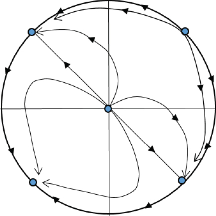
Global phase portrait for case 1 (12)

Case 2. If Δ = 0 then λ₁ = λ₂ > 0 that is, the origin is a repulsor critical point. For the points at infinity the system (14) is reduced to:

±y˙=(y−a−b)2±z˙=zy

with solution y = a + b > 0. Then the phase portrait for the system in this case is:

$Global phase portrait for case 2 (12)$

Global phase portrait for case 2 (12)

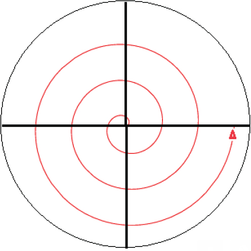
Case 3. If Δ < 0 then λ1=(a+b)+ic−2ab and λ2=(a+b)−ic−2ab with (a + b ) > 0 that is the origin is critical point of a spiral type. So the phase portrait for the system in this case is:

$Global phase portrait for case 3 (12)$

Global phase portrait for case 3 (12)

As regards infinity, the equation (15) has no real solutions, that is, it has no critical points at infinity.

4 Bifurcations

Lemma 4.1

Let B₀:= {(a,b,c ): a² + b² < − c}. if (a,b,c ) ∈ B₀then the associated system of the form (12) has unstable critical point (0, 0).

Proof

We consider eigenvalues (13), if (a,b, c ) ∈ B₀ that is a² + b² < − c, then (a + b )² < 2ab − c, it is 0<(a+b)<2ab−c

If a + b > 0, then a+b<2ab−c
λ2=a+b−2ab−c2<0 & λ1=a+b+2ab−c2>0.
This implies that the critical point (0, 0 ) is of a saddle type.
If a + b < 0, then −(a+b)<2ab−c, i.e.
λ1=a+b+2ab−c2>0 & λ2=a+b−2ab−c2<0.
Then the critical point (0, 0 ) is of a saddle type.
If a + b = 0 then λ1=2ab−c>0 and λ2=−2ab−c<0. Then the critical point (0, 0) is of a sadle type.

Lemma 4.2

Let B₁:= {(a,b,c): 2ab − c < 0 & a + b > 0}. if (a,b,c ) ∈ B₁then the associated system of the form (12)has unstable focus critical point (0, 0).

Proof

We consider the eigenvalues (13), if (a,b, c ) ∈ B₁, then 0 < (a + b )² > 0 > 2ab − c, i.e. that the eigenvalues are:

λ1=a+b+ic−2ab2<0 & λ2=a+b−ic−2a2<0.

where the real part in both cases is (a+ b ) > 0, i.e. the critical point is focus stable.

Lemma 4.3

Let B₂:= {(a,b,c): 2ab − c < 0 & a + b > 0}. If (a,b,c) ∈ B₂the associated system of the form (12) has a critical point of saddle type (0, 0).

Proof

The proof of this lemma is as in the previous lemma, but in this case a + b < 0, then the critical point is focus stable.

Lemma 4.4

Let B₃:= {(a,b,c ) : 2ab − c ≥ 0 & a + b > 0 & a² + b² > − c}. If (a,b,c ) ∈ B₃then the associated system of the form (12)has a critical point of unstable node type (0, 0).

Proof

We consider the eigenvalues (13), if (a,b, c ) ∈ B₃, then a² + b² > − c, that is (a + b )² > 2ab − c > 0, i.e.

λ1=a+b+2ab−c>0 & λ2=a+b−2ab−c>0.

Then the critical point (0, 0 ) is an unstable node.

Lemma 4.5

Let B₄:= {(a,b,c ): 2ab − c ≥ 0 & a + b < 0 & a² + b² > − c}. If (a,b,c ) ∈ B₄then the associated system of the form (12)has a critical point stable node type (0, 0).

Proof

If (a,b, c ) ∈ B₄, then |a+b|≥2ab−c, but a + b < 0 that is −(a+b)≥2ab−c. Now the eigenvalues are:

λ1=a+b+2ab−c<0 & λ2=a+b−2ab−c<0.

Then the critical point(0, 0 ) is a stable node.

Proposition 4.6

The set B := {(a,b,c ) :a + b < 0 & a² + b² = − c} ∪ {(a,b,c ) :a + b = 0 & a² + b² > − c} is a bifurcation for the system (12).

Proof

For the previous lemmas, the set B is a bifurcation for the family of systems (12).

Remark 4.7

The Proposition (4.6) us present a new kind of bifurcation.

The following corollary summarizes the study of the bifurcations for the rest of families and is a direct consequence of the proposition (4.6).

Corollary 4.8

The following statements hold:

For the family (4), c = 0 is a bifurcation. For the family (5) there is no bifurcation. For the family (6) a = 0 is a bifurcation.
For the families (7) and (8), the set F₁:= {(b, c ) : b = 0 & b² > − c or b² = − c & b > 0} is a bifurcation.
For the families (9) and (10), the set F₂:= {(a, c ) : a = 0 & a² > − c or a² = − c & a > 0} is a bifurcation.
For the family (11) the set F₃:= {(a,b): a + b = 0} is a bifurcation.

5 Galoisian aspects

To simplify the next proposition, we summarize all the possibilities for parameter ρ in Table 1.

Table 1

Possibles ρ values.

a	b	c	ρ	*Differential Galois Group*
0	0	≠ 0	− C	Gm
0	≠ 0	0	0	Ga
≠ 0	0	0	0	Ga
≠ 0	≠ 0	0	2ab	Gm
≠ 0	0	≠ 0	− C	Gm
0	≠ 0	≠ 0	− C	Gm
≠ 0	≠ 0	≠ 0	2ab − C	Gm

Proposition 5.1

For (12), with ρ = 2ab − c we have that:

If (2ab − c) = 0 then the differential Galois group is
DGal<L/K>=({σc:σc(y)=y+c c∈C},o)(1)
If (2ab − c) ≠ 0 then the differential Galois group is
DGal<L/K>=({σc/σc(y)=cy c∈C},o)(2)

Proof

The associated foliation to (12) is:

yy′=(2a+2b)y−(a2+c+b2)x.

Then taking into account that f(x) = −2(a + b )y and g (x) = (a² + c + b²)x, the Lienard equation will be:

x¨−(2a+2b)x˙+(a2+c+b2)x=0.

This is a second order equation with constant coefficients.

If we take it to the form ÿ = ρy with the change of variable x = exp(−1/2 ∫ f (x)dt) that is to say x = exp((a + b )t)y, we obtain:

y¨=(2ab−c)y.

Let’s analyze each case of the solution of the associated Lienard equation taking into account the following: (2ab − c ) = ρ . The solution of the second order reduced equation is y(t)=C1exp(ρt)+C2exp(−ρt) if they are taken (C₁,C₂) = (1, 0) or (C₁,C₂) = (0, 1) and the particular solutions are

y1=exp(ρt) y2=exp(−ρt).

With these we can build the solutions of the Lienard equation that are

x1=exp((a+b)t) x2=exp((a+b+2ab−c)t).

For these we have the following cases:

Case 1. If a,b,c ∈ C and (a+b+2ab−c)=α+iβ=z, then x₁ = exp(αt ). exp(βt)

1.1 If α ≥ 0 and β = 0 then x₁ is not bounded in −∞ and is not bounded in +∞
1.2 If α < 0 and β = 0 then x₁ is not bounded in +∞ and not bounded in −∞
1.3 If α = 0 and β ≠ 0 then the solution x₁ is periodic.

Case 2. If a,b,c ∈ R then x1=exp((a+b)t).exp(2ab−ct)

2.1 If c > 2ab then we will have two solutions x₁ and x₂.
2.2 If c > 2ab then (a+b)+2abc=(a+b)+ic−2ab, that is to say that we would be in case one with α = a + b, β=c−2ab and also if a = − b ⇒ α = 0 or a < − b ⇒ α < 0 and a > − b ⇒ α 0.

Our next aim will be to calculate the Galois groups associated with the equation ÿ = ρy, taking as a field of constants K = C . This study can be seen in [15]. We must consider two cases:

Case 1. If ρ = 0 then we will have the equation ÿ = 0, whose space of solutions is generated by y₁ = 1 and y₂ = t. The Picard-Vessiot extension is L = C < t >, where <t>={k^0+k^1t:k^0,k^1∈C}. If we take the automorphism σ ∈ DGal < L/K > we check what form we should have.
First we must consider that σ: L → L so that σ|_t = identity, then σ (y₁) = 1 = y₁. Now
σ(∂tt)=∂t(σ(t))σ(1)=1=∂t(σ(t))
Solving this equation by separable variables we have σ(t) = t + C . Therefore, the differential Galois group will be
DGal<L/K>=({σc:σc(y)=y+c c∈C},o)=Ga.
We can also see that:
σ(y1y2)=(10c11)
That is the differential Galois group is isomorphic to the group:
{(10c11):c∈C},•}
case 2. If ρ ≠ 0 we will then have the equation (ÿ) = ρy, taking the same field of constants from the previous case K. The base solutions for the equation are y1=expρt and y2=exp(−ρt)=1y1. The Picard-Vessiot extension will be L=C<exp(ρt)>.
Now suppose that σ ∈ DGal < L /K > and let’s see what action it performs on the solutions y₁,y₂.
σ(y1)=σ(exp(ρt))⇔∂tσ(y1)=σ(∂texp(ρt))=ρ(y1)
Solving the differential equation: ∂tσ(y1)=ρ(σ(y1)), by the method of separation of variables we have σ(y₁) = y₁.C. also as y₂ = 1/y₁, then σ(y2)=1σ(y1)=1c.y1=1cy2.
The Galois differential group will be
DGal<L/K>=({σc/σc(y)=cy c∈C},o)=Gm.
We can also see in this case that:
σ(y1y2)=(c001/c)
That is the Galois differential group is isomorphic to the group:
{(c001/c):c∈C,•}

6 Darboux theory of integrability

Proposition 6.1

Consider the values of ρ according to the table 1. The following statements hold:

The invariant algebraic curves aref1=−v+ρyf2=−v−ρand their respective generalized cofactorsK1=−1(v+ρ)yK2=−1(v−ρ).
The Generalized Exponential factors areF1(v,x)=exp(ρx+c)andF2(v,x)=exp(−ρx+c). Moreover, their respective generalized cofactors areL1=(v,x)=ρyL2=−ρ
The integrating factors areR1(v,x)=exp(−2ρx)(−v+ρ)2andR2(v,x)=exp(2ρx)(−v−ρ)2
The first integrals are given by
I1(v,x)=−v−ρ−exp(−2ρx)−2ρexp(−2ρx+C)−v−ρ(−2ρexp(−2ρx))exp(1/4ρ)I2(v,x)=−v+ρ−exp(2ρx)2ρexp(2ρx)+C−v+ρ(2ρexp(2ρx))exp(1/4ρ)

Proof

If we change the variable v=y˙y about the equation ÿ = ρy we will have the Riccati equation:

v˙=ρ−v2,

with solutions corresponding to y₁,y₂, respectively,

v1=ρ, v2=−ρ.

Taking this equation as a foliation, the associated system will be:

x˙=1v˙=ρ−v2(16)

and the associated vector field is X ∂_x + (ρ − V²)∂_v.

Applying Lemma 1 of [3], we identify each of the Darboux integrability elements (also defined in Section 1.2), with v_λ(x) as the solution:

Invariant Algebraic Curves:
(f_λ(v, x ) = − v + v_λ(x))
f1=−v+ρ and f2=−v−ρ
Generalized Cofactors:
(K_λ(v, x ) = − N(x)(v + v_λ (x))) in this case:
K1=−1(v+ρ) and k2=−1(v−ρ)
Generalized Exponential Factor:
Fλ(v,x)=exp∫(N′(x)2N(n)+vλ(x))dx in this case:
F1(v,x)=exp(∫(02+v1(x))dx)=exp(∫ρdx)=exp(ρx+c)
also
F2(v,x)=exp(∫(02+v2(x))dx)=exp(∫−ρdx)=exp(−ρx+c)
Generalized Cofactor:
L_λ(v, x ) = N′(x)/2 + N (x) v_λ(x), in this case:
L1=(v,x)=N′/2+Nv1=ρ, L2=(v,x)=N′/2+Nv2=−ρ
Integrating Factor:
Rλ(v,x)=exp(∫(−N′/N−2vλ)dx)−v+vλ
R1(v,x)=exp(∫(−1′/1−2v1)dx)−v+v1=exp(−2ρx)(−v+ρ)2,R2(v,x)=exp(∫(−1′/1−2v2)dx)−v+v2=exp(2ρx)(−v−ρ)2.
First Integral For this case we must first calculate two elements:
1. v_(λ,1) = (ln(y_λ))′, in our case
  v(1,1)=ρ and v(2,1)=ρ
2. v(λ,2)=v(λ,1)+exp(−2∫v(λ,1)dx)∫(exp(−2∫v(λ,1)dx))dx, In our case
v(1,2)=v(1,1)+exp−2∫v(1,1)dx∫(exp(−2∫v(1,1)dx))dx=ρ+exp(−2∫ρdx)∫(exp(−2∫ρdx))dx=ρ−exp(−2ρx)−2ρexp(−2ρx)+Cv(2,2)=v(2,1)+exp(−2∫v(2,1)dx)∫(exp(−2∫v(2,1)dx))dx=−ρ+exp(2∫ρdx)∫(exp(2∫ρdx))dx=−ρ+exp(2ρx)2ρexp(2ρx)+C
Now the first integrals are given by:
Iλ(v,x)=−v−v(λ,2)−v−v(λ,1)exp(∫(v(λ,2)−v(λ,1))dx).
Then:
I1(v,x)=−v−ρ−exp⁡(−2ρx)−2ρexp⁡(−2ρx)+C−v−ρexp⁡(∫(ρ−exp⁡(−2ρx)−2ρexp⁡(−2ρx)+C−ρ)dx)=−v−ρ−exp⁡(−2ρx)−2ρexp⁡(−2ρx)+C−v−ρ(−2ρexp⁡(−2ρx))exp⁡(1/4ρ)I2(v,x)=−v+ρ−exp⁡(2ρx)2ρexp⁡(2ρx)+C−v+ρexp⁡(∫(−ρ+exp⁡(2ρx)2ρexp⁡(2ρx)+C+ρ)dx)=−v+ρ−exp⁡(2ρx)2ρexp⁡(2ρx)+C−v+ρ(2ρexp⁡(2ρx))exp⁡(1/4ρ)

7 Final remarks

In this paper we studied one parametric family of linear differential systems from algebraic and qualitative point of view. Such parametric family comes from the correction of Exercise 11 in [2, §1.3.3], which we called Polyanin-Zaitsev vector field, see [1].

In this case we have taken a particular member of a family of equations, which were studied in general case in [1]. We have found critical points and the description near to these points. To our knowledge, we have obtained a new type of bifurcation. In the algebraic approach, the explicit first integral has been found using the Darboux method. Moreover, the differential Galois groups associated to solutions have also been found.

References

[1] Acosta-Humánez P.B., Reyes-Linero A., Rodríguez-Contreras J., Algebraic and qualitative remarks about the family yy (αX^{m + k − 1} + βX^m−k−1)y + γX^2m−2k−1, preprint 2014. Available at arXiv:1807.03551.Search in Google Scholar

[2] Polyanin A.D., Zaitsev V.F., Handbook of exact solutions for ordinary differential equations, Second Edition, 2003, Chapman and Hall, Boca Raton.10.1201/9781420035339Search in Google Scholar

[3] Acosta-Humánez P.B., Pantazi Ch., Darboux Integrals for Schrodinger Planar Vector Fields via Darboux Transformations SIGMA, 2012, 8, 043.10.3842/SIGMA.2012.043Search in Google Scholar

[4] Van der Pol B., Van der Mark J., Frequency demultiplication, Nature, 1927, 120, 363–364.10.1038/120363a0Search in Google Scholar

[5] Nagumo J., Arimoto S., Yoshizawa S. An active pulse transmission line simulating nerve axon, Proc. IRE, 1962, 50, 2061–2070.10.1109/JRPROC.1962.288235Search in Google Scholar

[6] Guckenheimer J., Hoffman K., Weckesser W., The forced Van der Pol equation I: The slow flow and its bifurcations, SIAM J. Applied Dynamical Systems, 2003, 2, 1–35.10.1137/S1111111102404738Search in Google Scholar

[7] Kapitaniak T., Chaos for Engineers: Theory, Applications and Control, 1998, Springer, Berlin, Germany.10.1007/978-3-642-97719-0Search in Google Scholar

[8] Acosta-Humánez P.B., Lázaro J.T., Morales-Ruiz J.J., Pantazi Ch., On the integrability of polynomial fields in the plane by means of Picard-Vessiot theory. Discrete and Continuous Dynamical Systems, 2015, 35, 1767–180010.3934/dcds.2015.35.1767Search in Google Scholar

[9] Perko L., Differential equations and Dynamical systems, Third Edition, 2001, Springer-Verlag New York, Inc.10.1007/978-1-4613-0003-8Search in Google Scholar

[10] Guckenheimer J., Nonlinear Oscillations, Dynamical Systems and Bifurcations of Vector Fields, 1983, Springer-Verlag New York.10.1007/978-1-4612-1140-2Search in Google Scholar

[11] Nemytskii V.V., Stepanov V.V., Qualitative Theory of Differential Equations, 1960, Princeton University Press, Princeton.10.1515/9781400875955Search in Google Scholar

[12] Christopher C., Llibre J., Integrability via invariant algebraic curves for planar polynomial differential systems, Annals of Differential Equations, 2000, 14, 5–19.Search in Google Scholar

[13] Pantazi Ch., Inverse problems of the Darboux Theory of integrability for planar polynomial differential systems, PhD, 2004.Search in Google Scholar

[14] Acosta-Humánez P.B., Teoría de Morales-Ramis y el algoritmo de Kovacic, Lecturas Matemáticas. Volumen Especial, 2006, 21–56.Search in Google Scholar

[15] Acosta-Humánez P.B., Galoisian Approach to Supersymmetric Quantum Mechanics. PHD Thesis, Barcelona, 2009. Available at arXiv:0906.3532Search in Google Scholar

[16] Acosta-Humánez P., Morales-Ruiz J., Weil J.-A., Galoisian Approach to integrability of Schrödinger Equation. Reports on Mathematical Physics, 2011, 67, 305–374.10.1016/S0034-4877(11)60019-0Search in Google Scholar

[17] Acosta-Humánez P.B., Perez J., Teoría de Galois diferencial: una aproximación Matemáticas: Enseñanza Universitaria, 15, 2007, 91–102.Search in Google Scholar

[18] Acosta-Humánez P.B., Perez J., Una introducción a la teoría de Galois diferencial. Boletín de Matemáticas Nueva Serie, 2004, 11, 138–149.Search in Google Scholar

[19] van der Put M., Singer M., Galois Theory in Linear Differential Equations, 2003, Springer-Verlag New York.10.1007/978-3-642-55750-7Search in Google Scholar

[20] Morales-Ruiz J., Differential Galois Theory and Non-Integrability of Hamiltonian Systems, 1999, Birkhäuser, Basel.10.1007/978-3-0348-0723-4Search in Google Scholar

[21] Lang S., Linear Algebra, Undergraduate Text in Mathematics, 2010, Springer, Third edition.Search in Google Scholar

[22] Weil J.A., Constant et polynómes de Darboux en algèbre différentielle: applications aux systemes différentiels linéaires. Doctoral thesis, 1995.Search in Google Scholar

[23] Pantazi Ch., El metodo de Darboux, en notas del primer seminario de Integrabiliad. Universidad Politecnica de Catalunya, 2005. Available at https://upcommons.upc.edu/e − prints/bitstream/2117/2233/1/noinupc.pdf.Search in Google Scholar

[24] Giacomini H., Gine J., Grau M., Integrability of planar polynomial differential systems through linear differential equations. Birkhauser, Rocky Mountain J. Math., 2006, 36, 457–485.10.1216/rmjm/1181069462Search in Google Scholar

Received: 2018-03-07

Accepted: 2018-06-13

Published Online: 2018-10-31

This work is licensed under the Creative Commons Attribution-NonCommercial-NoDerivatives 4.0 License.

Articles in the same Issue

https://doi.org/10.1515/math-2018-0102

Keywords for this article

Integrability; Qualitative; Stability; Critical point; Polynomial; Polyanin-Zaitsev vector field

Creative Commons

BY-NC-ND 4.0