Global stability of a distributed delayed viral model with general incidence rate
-
 ,
,

Abstract
In this paper, we discussed a infinitely distributed delayed viral infection model with nonlinear immune response and general incidence rate. We proved the existence and uniqueness of the equilibria. By using the Lyapunov functional and LaSalle invariance principle, we obtained the conditions of global stabilities of the infection-free equilibrium, the immune-exhausted equilibrium and the endemic equilibrium. Numerical simulations are given to verify the analytical results.
1 Introduction
During recent decades there has been a lot of research regarding mathematical modelling of viruses’ dynamics via models of ordinary differential equations. The advances in immunology have lead us to better understand the interactions between populations of virus and the immune system, therefore several nonlinear sytems of ordinary differential equations have been proposed. Nowak and Bengham [1] study the model
Where x(t) denotes the number of healthy cells, y(t) denotes the infected cells, v(t) denotes the number of mature viruses and z(t) denotes the number of CTL (cytotoxic T lymphocyte response) cells. Uninfected target cells are assumed to be generated at a constant rate s and die at rate d. Infection of target cells by free virus is assumed to occur at rate β. Infected cells die at rate a and are removed at rate p by the CTL immune response. New virus is produced from infected cells at rate k and dies at rate u. The average lifetime of uninfected cells, infected cells and free virus is thus given by 1/d, 1/a and 1/u, respectively. The parameter c denotes the rate at which the CTL response is produced and b denotes death rate of the CTL response. All given constants are assumed to be positive.
Generally, the type of incidence function used in a model has an important role in modeling the dynamics of viruses. The most common, is the bilinear incidence rate βxv. However, this rate is not useful all the time. For instance, bilinear incidence suggests, that the model can not describe the infection process of hepatitis B, where individuals with small liver are more resistant to infection than the ones with a bigger liver. Recently, works about models of infections by viruses have used the incidence function of type Beddington-DeAngelis and Crowley-Martin. In [2] the authors propose a model of infection by virus with Crowley-Martin functional response
They construct a Lyapunov functional to establish the global dynamics of the system. More recently, in [4], the authors consider the system
They also give also results of global stability as well as, Hopf bifurcation results.
Yang and Wei in [5] consider a more general incidence rate, they study the system
giving some results about global stability in terms of the basic reproduction number and the immune response reproduction number. Here the f(v) is assumed to be a continuous function on v that belongs to (0, ∞) and satisfies f(0) = 0, f′(v) > 0 for all v greater or equal to 0 and f″(v) < 0 for all v greater or equal to 0.
In [6], the authors consider a more general incidence rate f(x, y, v)v, where f is assumed to be continuously differentiable in the interior of
f(0, y, v) = 0, for all y ≥ 0, v ≥ 0.
In [7], authors analyze an infection model by virus, with general incidence and immune response, which generalizes the systems [2, 6, 8], namely,
where f(x, y, v) is a continuous and differentiable function in the interior of
Another viral infection model is the studied in [9] given by:
Where x, y, v, z denotes the non infected cells, infected cells, virus and specific virus CTL at time t respectively. Conditions on functions fi, h, w, and gi are specified in [9]. Related works are [10, 11, 12, 13, 14].
Based on the discussion above, we will study a delayed viral infection model with general incidence rate and CTL immune response given by
The dynamics of uninfected cells, x, in the absence of infection is governed by x′ = n(x). n(x) is the intrinsic growth rate of uninfected cells accounting for both productions and natural mortality. This is assumed to satisfy the following:
n(x) is continuously differentiable, and exist x̄ > 0 such as that n(x̄) = 0, n(x) > 0 for x ∈ [0, x̄), and n(x) < 0 for x < x̄. Typical functions appearing in the literature are n(x) = s − dx and n(x) = s − dx + rx(1 − x/xmax).
φi is strictly increasing on [0, ∞); φi(0) = 0;
w(y, z) is continuously differentiable;
All parameters are nonnegative and the distributions fi for i = 1, 2 are assumed to satisfy the following (see [9, 14]):
fi(τ) ≥ 0, for τ ≥ 0.
In addition, the uniqueness and global stability results on the positive equilibrium require the following assumption:
w(y, z) = φ1(y)φ2(z).
In this paper, we will study the global dynamics model of (17)-(20). Organization is as follows: in section 2, we prove the existence and uniqueness of the infection free equilibrium, the CTL-inactivated infection equilibrium and the CTL-activated infection equilibrium. In section 3, the conditions that allow the global stability of each equilibrium are determined and proved. Section 4, provide several numerical simulations that show the results obtained in section 3 and 4. Finally, in section 5 we summarize the results we have obtained, comparing them with previous models studied in literature, and setting the guidelines for possible future work.
1.1 Positivity and boundedness
For system (17) the suitable space is 𝓒4 = 𝓒 × 𝓒 × 𝓒 × 𝓒, where 𝓒 is the Banach space of fading memory type ([15]):
where the norm of a ϕ ∈ 𝓒 is defined as ∥ϕ∥ = supθ≤0 ∣ϕ(θ)∣eαθ. The nonnegative cone of 𝓒 is defined as 𝓒+ = C((−∞, 0], ℝ+).
Theorem 1.1
Under the initial conditions, all solutions of system(17)-(20)are positive and ultimately uniformly bounded inX.
Proof
To see that x(t) is positive, we proceed by contradiction. Let t1 the first value of time such that x(t1) = 0. From (17) we see that x′(t1) = n(0) > 0 and x(t1) = 0, therefore there exists ϵ > 0 such that x(t) < 0 for t ∈ (t1 − ϵ, t1), this leads to a contradiction. It follows that x(t) is always positive. With a similar argument we see that y(t), v(t) and z(t) are positive for t ≥ 0.
The hypotheses (H1) and equation (17) imply that limsupt⟶∞x(t) ≤ x̄.
From (17), (18) and assumption (H2), we obtain
where M1 = supx∈[0,x̄]n(x) and G1 =
Let e(t) =
and thus limsupt⟶∞ (e(t) + y(t))
where
Using a similar argument, let G3 =
and
therefore limsupt⟶∞L(t)
Therefore, x(t), y(t), v(t) and z(t) are ultimately uniformly bounded in 𝓒4. □
Previous theorem implies that the omega limit set of system (17)-(20) is contained in the following bounded feasible region:
It can be verified that the region Γ is positively invariant with respect to model (17)-(20) and that the model is well posed.
2 Existence and uniqueness of equilibria of system
At any equilibrium we have
System (17)-(20) always has an infection free equilibrium E0 = (x̄, 0, 0, 0). In addition to E0, the system could have two types of chronic infection equilibria E1 = (x1, y1, v1, 0) and E2 = (x2, y2, v2, z2) in Γ, where the entries of E1 and E2 are strictly positive. The equilibria E1 and E2 are called CTL-inactivated infection equilibrium (CTL-IE) and CTL-activated infection equilibrium (CTL-AE), respectively.
We define the general reproduction number as
which is the ratio of the per capita production and decay rates of mature viruses at an equilibrium (x, y, v, z) with z = 0. In particular, at the infection free equilibrium, E0, we denote R(x̄, 0, 0) by R0, representing the basic production number for viral infection:
From assumption (H2) we have that φ1 is invertible, so we can define from equation (25):
Define also H(x) = n(x) − f(x, ŷ, v̂)v̂, we have H(0) = n(0) > 0 and H(x̄) = − f(x̄, ŷ, v̂)v̂, with f(x̄, ŷ, v̂) > f(0, ŷ, v̂) = 0 by (ii), so there exists a x̂ ∈ (0, x̄) such that H(x̂) = 0. We denote:
and refer it as the viral reproduction number. From assumptions on f it is easy to see that f(x̄, 0, 0) > f(x̄, y, v), for all y, v > 0, moreover for all x ∈ [0, x̄) we have f(x, y, v) < f(x̄, y, v), so:
Particularly, R0 > R1. The basic reproduction number for the CTL response is given by:
In order to prove of the existence and uniqueness of equilibria, we require two additional assumptions. First, we define the following sets:
The following conditions are used to guarantee the uniqueness of the equilibria.
The system (17) has an equilibrium E2 = (x2, y2, v2, z2) satisfying Xn ∩ Xf(y2, v2).
Theorem 2.1
Assume that i) − iii) andH1 − H4are satisfied.
IfR0 > R1 > 1 then, in addition toE0andE1system(17)has a CTL activated infection equilibrium.
When x = x̄ and y = v = z = 0 the equations (22)-(25)are satisfied, therefore E0 = (x0, 0, 0, 0) is a steady state called the infection free equilibrium. To prove that it is unique when R0 < 1, we look for the existence of a positive equilibrium.
To find a positive equilibrium we proceed as follows: from equation (25)φ2(z) = 0 or φ1(y) =
By (H2), we know that
with ϕ(x̄) = 0 and ϕ(0) = y0 being a unique root of equations
Note that, from (ii) we have f(x, y, v) > f(0, y, v) = 0, ∀x > 0. So if E* = (x*, y*, v*, z*) is a positive equilibrium, then n(x*) = f(x*, y*, v*)v* > 0, so x* ∈ (0, x̄).
Now, using (29) define on the interval [0, x̄) the function G,
we have
or equivalently
We conclude that, for R0 > 1, there exists another equilibrium E1 = (x1, y1, v1, 0) with x1 = x* ∈ (0, x̄), y1 = ϕ(x1) and
so equation (22) never holds. Therefore, E1 exists iff R0 > 1.
Next we show that E1 = (x1, y1, v1, 0) is unique. Suppose, to the contrary, that there exists another CTL-IE equilibrium
Note that the CTL-AE E2 = (x2, y2, v2, z2) exists if (x2, y2, v2, z2) ∈
Note that the values x̂, ŷ, v̂ are used to define R1, so they clearly satisfy the equilibrium equations. Solving the equation (23) for z and using (H2) yields
Now we will prove that E2 is unique. Suppose that there exists another CTL-AE,
3 Global stability
Let R0 and R1 be defined as in previous section.
Theorem 3.1
IfR0 < 1, then infection free-EquilibriumE0of model(17)-(20)is globally asymptotically stable.
Proof
Define a Lyapunov functional
where Gi =
Calculating the derivative of V1 along the positive solutions of system (17)-(20), it follows that
Using n(x0) = 0 and simplifying, we get
Using the following inequalities:
We have that
Since R0 ≤ 1, we have V̇1 ≤ 0. Therefore the disease free E1 is stable, V̇1 = 0 if and only if x = x0, y = 0, v = 0, z = 0. So, the largest compact invariant set in {(x, y, v, z):V̇1 = 0} is just the singleton E1. From LaSalle invariance principle, we conclude that E1 is globally asymptotically stable. □
Theorem 3.2
IfR0 > 1 andR1 < 1, then CTL-IEE1, of model (17) is globally asymptotically stable.
Proof
Consider the following Lyapunov functional:
where
At infected equilibrium
Calculating the derivative of L̂ along the positive solutions of (17), we get
Therefore
Using the inequalities:
We have that
Since R1 ≤ 1, we have V̇1 ≤ 0, thus E1 is stable. V̇1 = 0 if and only if x = x1, y = y1, v =1, z = 0. So, the largest compact invariant set in {(x, y, v, z) : v̇1 = 0} is the singleton E1. From LaSalle invariance principle, we conclude that E1 is globally asymptotically stable. □
Theorem 3.3
Assume that (i)−(iii), H1 − H4hold andf3(τ) = δ (τ). IfR1 > 1, then the CTL-AE, E2is Globally asymptotically stable.
Proof
Define a Lyapunov functional for E2.
The derivative of V2 along with the solutions of system (17) is
Applying n(x2) = f(x2, y2, v2)v2, f(x2, y2, v2)
Therefore
Therefore V̇2 ≤ 0, thus E2 is stable. V̇2 = 0 if and only if x = x2, y = y2, v = v2, z = z3. So, the largest compact invariant set in {(x, y, v, z) : V̇2 = 0} is the singleton E2. From LaSalle invariance principle, we conclude that E2 is globally asymptotically stable. □
4 Numerical simulations
In this section we present some numerical simulations to illustrate the results of stability, obtained in our theorems from previous sections.
Example 4.1
Consider the functions
Then, the model takes the form:
Fix the parameters as λ = 200, d = 0.1, r = 0.6, K = 500, p = 1, k = 0.8, α2 = 0.05, u = 3.5, c = 0.03, b = 0.75, τ1 = 5, τ2 = 10, μ = 0.1, α = γ = 0.001. The trivial equilibrium point is given byE0 = (666.6666, 0, 0, 0), so the basic reproduction number 𝓡0is obtained by:
𝓡0 ≤ 1 iffβ ≤ 0.009513986. We setβ = 0.003 . By Theorem 2.1 i), we have the single equilibriumE0 = (666.6666, 0, 0, 0) which is globally asymptotically stable by Theorem 3.1. Using a constant history functionS = (25, 50, 10, 5) fort ∈ (0, 10) and the tool DDE 23 from Matlab, we can compute numerically the solution of system(34)-(37)fort ∈ (10, 200). The results are shown in Figure 1, where we can see that the solution goes to the equilibria pointE0.
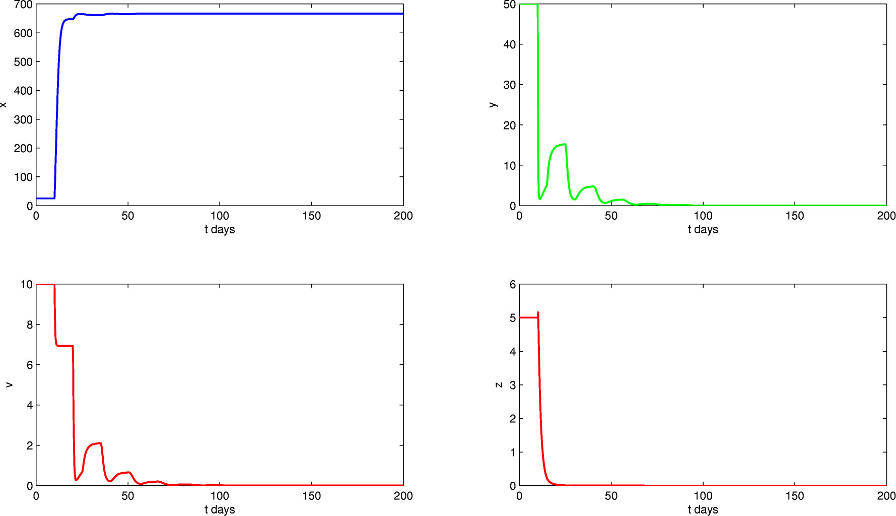
Global stability of infection free equilibrium for 𝓡0 < 1.
Example 4.2
Now, setβ = 0.0096, soR0 > 1. ComputingR1from its definition we haveR1 =
thereforeR1 = 0.97091 < 1 and we have then, a second equilibrium
Using the history function from previous example we can plot the solution with Matlab. By Theorem 3.2, E1is globally asymptotically stable as we can see in Figure 2.
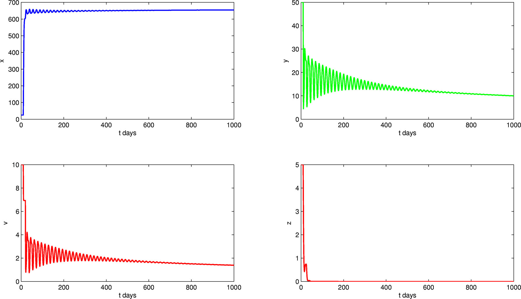
Global stability of CTL-IE E1 for 𝓡0 > 1 > R1.
Finally, forβ = 1, we haveR0 > 1 andR1 = 6.088529, so there exists an infection free equilibriumE0and two equilibria
and
By Theorem 3.3 we have global stability of equilibriumE2. We can see in Figure 3 that the solutions approach toE2.
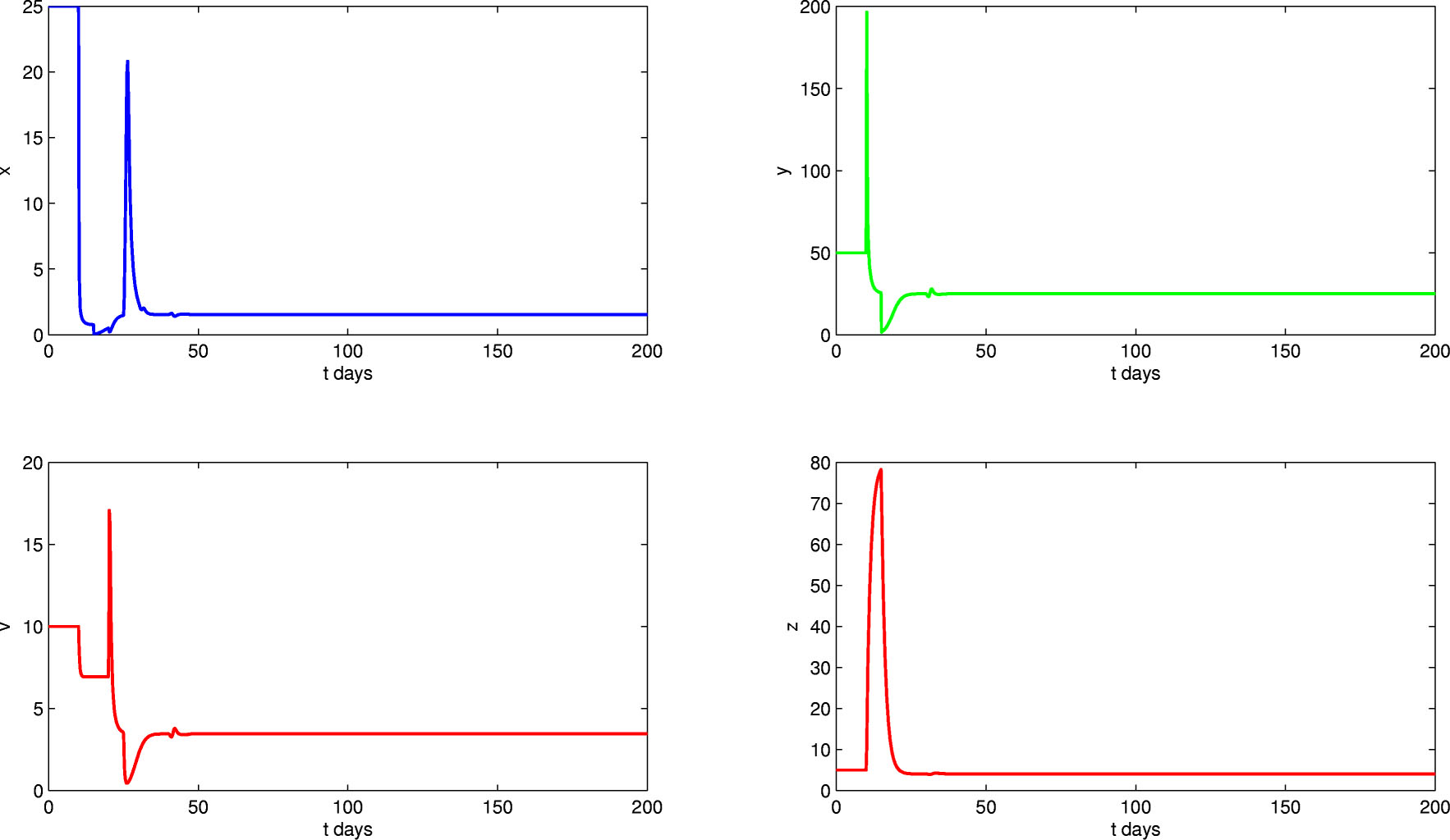
Global stability of CTL-AE E2 for R0 > 1, R1 > 1.
Example 4.3
In order to show that our model, generalizes the previous articles, we propose the following incidence function to show our results:
This function is not included in the cases studied by [9], since the general form in that work ish(x, v). Our functionfincludes the three variablesx, y, vand satisfies our conditions (i)-(iii) to be an admisible incidence rate.
f(0, y, v) = 0, ∀y, v ≥ 0.
Setting the other functions and parameters, as in Example 4.1, then we obtain model:
The infection free equilibrium isE0 = (666.6666, 0, 0, 0) as in previous cases, withR0 = 70.0722745 β, soR0 > 1 iffβ > 0.01427097. Therefore, if we setβ = 0.1 then we haveR0 > 1, R1 = 4.9234560677357286281 and there exists two more equilibria points,
withE2globally asymptotically stable. Figure 4 shows how the solutions approach to the equilibriumE2.
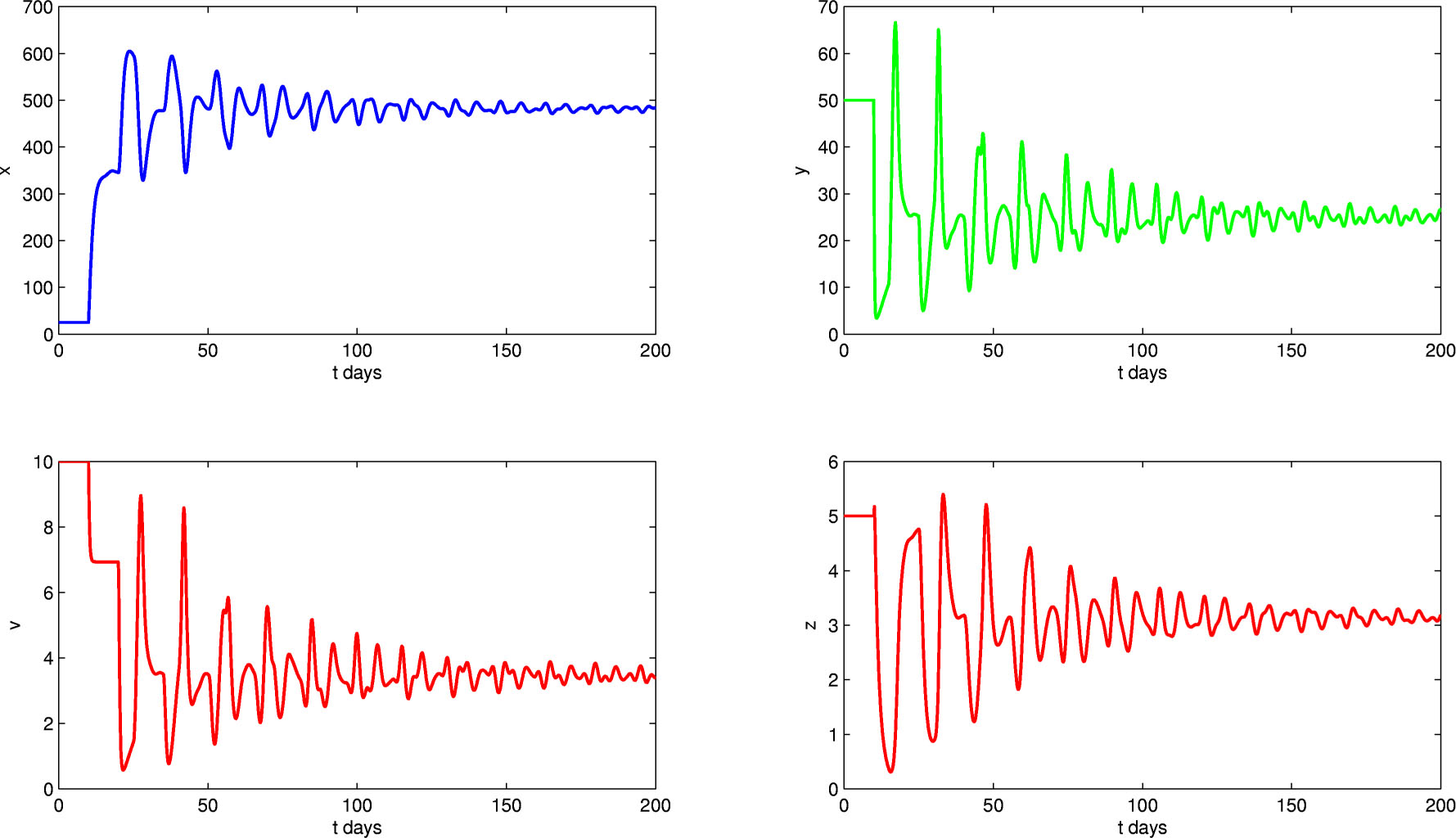
Global stability of CTL-AE E2 for
5 Conclusions
In this paper we studied the global properties of a model of infinitely distributed delayed viral infection. That considers a nonlinear CTL immune response, given by w(y, z) = ϕ1(y) ϕ2(z) and a general incidence function of the form f(x, y, v)v, where w and f satisfy certain conditions derived from previous works and biological meanings. Even when there exists variety of papers that include the CTL immune response (see for example [1, 3, 4, 5, 7]) and general incidence functions of various types (see [5, 7, 9]), the model proposed in this article includes a family of the works studied by several authors, and their conclusions can be seen as a particular case of our theorems. There lies its importance and relevance.
The model always presents an infection free positive equilibrium E0 = (x̄, 0, 0, 0), and two types of chronic infection equilibria: the CTL inactivated infection equilibrium (CTL-IE) E1 = (x1, y1, v1, 0) and the CTL activated infection equilibrium (CTL-AE) E2 = (x2, y2, v2, z2). The coexistence of these equilibria is determined by the basic reproduction number R0 and the viral reproduction number R1. These were defined in section 2 and are given in terms of parameters and the functions f(x, y, v), fi(τ), ϕ1(y) and ϕ2(z). The results show that R0 > R1 and the system admits always a positive infection free equilibrium E0, which is the unique equilibrium when R0 ≤ 1. If R0 > 1 which in addition to E0 provides only the CTL-IE (when R1 ≤ 1), or the coexistence of the CTL-IE and CTL-AE (R1 > 1).
We proved, by construction of a Lyapunov function, that whenever the equilibrium E0 is unique (R0 ≤ 1) and R0 ≠ 1, E0 is globally asymptotically stable. Moreover when R0 > 1 and R1 < 1 the CTL-IE, E1 is globally asymptotically stable. In the case of CTL-AE, E2 we obtained conditions for global stability only in the case f3(τ) = δ (τ), i.e., when the equation ż does not present delay. The results indicate that in this case, the equilibrium E2 is globally asymptotically stable when R1 > 1 and conditions (i)−(iii), H1 − H4 hold. It will be of interest to find conditions that guarantee the global stability of the E2 with a general f3(τ), this topic can be taken as a future work.
Acknowledgement
This article was supported in part by Mexican SNI under grant 15284 and CONACYT Scholarship 295308.
References
[1] Nowak M. A. and Bangham C. R. Population dynamics of immune responses to persistent viruses, Science, 1996, 272(5258), 74-79.10.1126/science.272.5258.74Search in Google Scholar PubMed
[2] Xu S. Global stability of the virus dynamics model with Crowley-Martin functional response. Electron. J. Qual. Theory of Differ. Eq., 2012, 9,1–10.10.14232/ejqtde.2012.1.9Search in Google Scholar
[3] Li X. and Fu S. Global stability of a virus dynamics model with intracellular delay and CTL immune response. Math. Methods Appl. Sci., 2015, 38(3), 420–430.10.1002/mma.3078Search in Google Scholar
[4] Yang Y. Stability and hopf bifurcation of a delayed virus infection model with Beddington–DeAngelis infection function and cytotoxic T-lymphocyte immune response. Math. Methods Appl. Sci., 2015, 38(18), 5253–5263.10.1002/mma.3455Search in Google Scholar
[5] Yang H. and Wei J. Analyzing global stability of a viral model with general incidence rate and cytotoxic T lymphocytes immune response. Nonlinear Dyn., 2015, 82(1-2), 713–722.10.1007/s11071-015-2189-8Search in Google Scholar
[6] Hattaf K., Yousfi N., and Tridane A. Mathematical analysis of a virus dynamics model with general incidence rate and cure rate. Nonlinear Anal. Real World Appl., 2012,13(4), 1866–1872.10.1016/j.nonrwa.2011.12.015Search in Google Scholar
[7] Hattaf K., Yousfi N., and Tridane A. Global stability analysis of a generalized virus dynamics model with the immune response. Can. Appl. Math. Q., 2012, 20(4), 499–518.Search in Google Scholar
[8] Wang X., Tao Y., and Song X. Global stability of a virus dynamics model with Beddington–DeAngelis incidence rate and CTL immune response. Nonlinear Dyn., 2011, 66(4), 825–830.10.1007/s11071-011-9954-0Search in Google Scholar
[9] Shu H., Wang L., and Watmough J. Global stability of a nonlinear viral infection model with infinitely distributed intracellular delays and CTL immune responses. SIAMJ. Appl. Math., 2013, 73(3), 1280–1302.10.1137/120896463Search in Google Scholar
[10] Hattaf K. and Yousfi N. A class of delayed viral infection models with general incidence rate and adaptive immune response. International Journal of Dynamics and Control, 2016, 4(3), 254–265.10.1007/s40435-015-0158-1Search in Google Scholar
[11] Ji Y. and Liu L. Global stability of a delayed viral infection model with nonlinear immune response and general incidence rate. Discrete & Continuous Dyn. Syst. Ser.B, 2016, 21(1).10.3934/dcdsb.2016.21.133Search in Google Scholar
[12] Wang J., Tian X., and Wang X. Stability analysis for delayed viral infection model with multitarget cells and general incidence rate. Int. J. Biomath., 2016, 9(01), 1650007.10.1142/S1793524516500078Search in Google Scholar
[13] Wang J., Lang J., and Li F. Constructing lyapunov functionals for a delayed viral infection model with multitarget cells, nonlinear incidence rate, state-dependent removal rate. J. Nonlinear Sci. Appl., 2016, 9, 524–536.10.22436/jnsa.009.02.18Search in Google Scholar
[14] Wang J., Guo M., Liu X., and Zhao Z. Threshold dynamics of HIV–1 virus model with cell-to-cell transmission, cell-mediated immune responses and distributed delay. Appl. Math. Comput., 2016, 291,149–161.10.1016/j.amc.2016.06.032Search in Google Scholar
[15] FV A. and Haddock J. On determining phase spaces for functional differential equations. Funkcialaj Ekvacioj, 1988, 31, 331–347.Search in Google Scholar
© 2018 Ávila-Vales et al., published by De Gruyter
This work is licensed under the Creative Commons Attribution-NonCommercial-NoDerivatives 4.0 License.
Articles in the same Issue
- Regular Articles
- Algebraic proofs for shallow water bi–Hamiltonian systems for three cocycle of the semi-direct product of Kac–Moody and Virasoro Lie algebras
- On a viscous two-fluid channel flow including evaporation
- Generation of pseudo-random numbers with the use of inverse chaotic transformation
- Singular Cauchy problem for the general Euler-Poisson-Darboux equation
- Ternary and n-ary f-distributive structures
- On the fine Simpson moduli spaces of 1-dimensional sheaves supported on plane quartics
- Evaluation of integrals with hypergeometric and logarithmic functions
- Bounded solutions of self-adjoint second order linear difference equations with periodic coeffients
- Oscillation of first order linear differential equations with several non-monotone delays
- Existence and regularity of mild solutions in some interpolation spaces for functional partial differential equations with nonlocal initial conditions
- The log-concavity of the q-derangement numbers of type B
- Generalized state maps and states on pseudo equality algebras
- Monotone subsequence via ultrapower
- Note on group irregularity strength of disconnected graphs
- On the security of the Courtois-Finiasz-Sendrier signature
- A further study on ordered regular equivalence relations in ordered semihypergroups
- On the structure vector field of a real hypersurface in complex quadric
- Rank relations between a {0, 1}-matrix and its complement
- Lie n superderivations and generalized Lie n superderivations of superalgebras
- Time parallelization scheme with an adaptive time step size for solving stiff initial value problems
- Stability problems and numerical integration on the Lie group SO(3) × R3 × R3
- On some fixed point results for (s, p, α)-contractive mappings in b-metric-like spaces and applications to integral equations
- On algebraic characterization of SSC of the Jahangir’s graph 𝓙n,m
- A greedy algorithm for interval greedoids
- On nonlinear evolution equation of second order in Banach spaces
- A primal-dual approach of weak vector equilibrium problems
- On new strong versions of Browder type theorems
- A Geršgorin-type eigenvalue localization set with n parameters for stochastic matrices
- Restriction conditions on PL(7, 2) codes (3 ≤ |𝓖i| ≤ 7)
- Singular integrals with variable kernel and fractional differentiation in homogeneous Morrey-Herz-type Hardy spaces with variable exponents
- Introduction to disoriented knot theory
- Restricted triangulation on circulant graphs
- Boundedness control sets for linear systems on Lie groups
- Chen’s inequalities for submanifolds in (κ, μ)-contact space form with a semi-symmetric metric connection
- Disjointed sum of products by a novel technique of orthogonalizing ORing
- A parametric linearizing approach for quadratically inequality constrained quadratic programs
- Generalizations of Steffensen’s inequality via the extension of Montgomery identity
- Vector fields satisfying the barycenter property
- On the freeness of hypersurface arrangements consisting of hyperplanes and spheres
- Biderivations of the higher rank Witt algebra without anti-symmetric condition
- Some remarks on spectra of nuclear operators
- Recursive interpolating sequences
- Involutory biquandles and singular knots and links
- Constacyclic codes over 𝔽pm[u1, u2,⋯,uk]/〈 ui2 = ui, uiuj = ujui〉
- Topological entropy for positively weak measure expansive shadowable maps
- Oscillation and non-oscillation of half-linear differential equations with coeffcients determined by functions having mean values
- On 𝓠-regular semigroups
- One kind power mean of the hybrid Gauss sums
- A reduced space branch and bound algorithm for a class of sum of ratios problems
- Some recurrence formulas for the Hermite polynomials and their squares
- A relaxed block splitting preconditioner for complex symmetric indefinite linear systems
- On f - prime radical in ordered semigroups
- Positive solutions of semipositone singular fractional differential systems with a parameter and integral boundary conditions
- Disjoint hypercyclicity equals disjoint supercyclicity for families of Taylor-type operators
- A stochastic differential game of low carbon technology sharing in collaborative innovation system of superior enterprises and inferior enterprises under uncertain environment
- Dynamic behavior analysis of a prey-predator model with ratio-dependent Monod-Haldane functional response
- The points and diameters of quantales
- Directed colimits of some flatness properties and purity of epimorphisms in S-posets
- Super (a, d)-H-antimagic labeling of subdivided graphs
- On the power sum problem of Lucas polynomials and its divisible property
- Existence of solutions for a shear thickening fluid-particle system with non-Newtonian potential
- On generalized P-reducible Finsler manifolds
- On Banach and Kuratowski Theorem, K-Lusin sets and strong sequences
- On the boundedness of square function generated by the Bessel differential operator in weighted Lebesque Lp,α spaces
- On the different kinds of separability of the space of Borel functions
- Curves in the Lorentz-Minkowski plane: elasticae, catenaries and grim-reapers
- Functional analysis method for the M/G/1 queueing model with single working vacation
- Existence of asymptotically periodic solutions for semilinear evolution equations with nonlocal initial conditions
- The existence of solutions to certain type of nonlinear difference-differential equations
- Domination in 4-regular Knödel graphs
- Stepanov-like pseudo almost periodic functions on time scales and applications to dynamic equations with delay
- Algebras of right ample semigroups
- Random attractors for stochastic retarded reaction-diffusion equations with multiplicative white noise on unbounded domains
- Nontrivial periodic solutions to delay difference equations via Morse theory
- A note on the three-way generalization of the Jordan canonical form
- On some varieties of ai-semirings satisfying xp+1 ≈ x
- Abstract-valued Orlicz spaces of range-varying type
- On the recursive properties of one kind hybrid power mean involving two-term exponential sums and Gauss sums
- Arithmetic of generalized Dedekind sums and their modularity
- Multipreconditioned GMRES for simulating stochastic automata networks
- Regularization and error estimates for an inverse heat problem under the conformable derivative
- Transitivity of the εm-relation on (m-idempotent) hyperrings
- Learning Bayesian networks based on bi-velocity discrete particle swarm optimization with mutation operator
- Simultaneous prediction in the generalized linear model
- Two asymptotic expansions for gamma function developed by Windschitl’s formula
- State maps on semihoops
- 𝓜𝓝-convergence and lim-inf𝓜-convergence in partially ordered sets
- Stability and convergence of a local discontinuous Galerkin finite element method for the general Lax equation
- New topology in residuated lattices
- Optimality and duality in set-valued optimization utilizing limit sets
- An improved Schwarz Lemma at the boundary
- Initial layer problem of the Boussinesq system for Rayleigh-Bénard convection with infinite Prandtl number limit
- Toeplitz matrices whose elements are coefficients of Bazilevič functions
- Epi-mild normality
- Nonlinear elastic beam problems with the parameter near resonance
- Orlicz difference bodies
- The Picard group of Brauer-Severi varieties
- Galoisian and qualitative approaches to linear Polyanin-Zaitsev vector fields
- Weak group inverse
- Infinite growth of solutions of second order complex differential equation
- Semi-Hurewicz-Type properties in ditopological texture spaces
- Chaos and bifurcation in the controlled chaotic system
- Translatability and translatable semigroups
- Sharp bounds for partition dimension of generalized Möbius ladders
- Uniqueness theorems for L-functions in the extended Selberg class
- An effective algorithm for globally solving quadratic programs using parametric linearization technique
- Bounds of Strong EMT Strength for certain Subdivision of Star and Bistar
- On categorical aspects of S -quantales
- On the algebraicity of coefficients of half-integral weight mock modular forms
- Dunkl analogue of Szász-mirakjan operators of blending type
- Majorization, “useful” Csiszár divergence and “useful” Zipf-Mandelbrot law
- Global stability of a distributed delayed viral model with general incidence rate
- Analyzing a generalized pest-natural enemy model with nonlinear impulsive control
- Boundary value problems of a discrete generalized beam equation via variational methods
- Common fixed point theorem of six self-mappings in Menger spaces using (CLRST) property
- Periodic and subharmonic solutions for a 2nth-order p-Laplacian difference equation containing both advances and retardations
- Spectrum of free-form Sudoku graphs
- Regularity of fuzzy convergence spaces
- The well-posedness of solution to a compressible non-Newtonian fluid with self-gravitational potential
- On further refinements for Young inequalities
- Pretty good state transfer on 1-sum of star graphs
- On a conjecture about generalized Q-recurrence
- Univariate approximating schemes and their non-tensor product generalization
- Multi-term fractional differential equations with nonlocal boundary conditions
- Homoclinic and heteroclinic solutions to a hepatitis C evolution model
- Regularity of one-sided multilinear fractional maximal functions
- Galois connections between sets of paths and closure operators in simple graphs
- KGSA: A Gravitational Search Algorithm for Multimodal Optimization based on K-Means Niching Technique and a Novel Elitism Strategy
- θ-type Calderón-Zygmund Operators and Commutators in Variable Exponents Herz space
- An integral that counts the zeros of a function
- On rough sets induced by fuzzy relations approach in semigroups
- Computational uncertainty quantification for random non-autonomous second order linear differential equations via adapted gPC: a comparative case study with random Fröbenius method and Monte Carlo simulation
- The fourth order strongly noncanonical operators
- Topical Issue on Cyber-security Mathematics
- Review of Cryptographic Schemes applied to Remote Electronic Voting systems: remaining challenges and the upcoming post-quantum paradigm
- Linearity in decimation-based generators: an improved cryptanalysis on the shrinking generator
- On dynamic network security: A random decentering algorithm on graphs