Restricted triangulation on circulant graphs

Lemma 2.1

If T_n is a restricted triangulation of a circulant graph G = C(n, S), then S contains D(T_n).

Proof

Suppose T_n is a restricted triangulation of G = C(n, S). Let d ∈ D(T_n). By definition of span of edges, there is an edge v_iv_j in T_n such that v_iv_j = v_iv_{i± d} where d = min{|j − i|, n − |j − i|}. Since T_n is a restricted triangulation of G, then E(T_n) ⊂ E(G). Hence, v_iv_{i ± d} ∈ E(G). Thus, d∈ S (by definition of S) □

The following proposition proves that any circulant graph C(n, S) does not admit a restricted triangulation unless 1, 2 ∈ S.

Proposition 2.2

Let n ≥ 4 be a natural number. Suppose the circulant graph C(n, S) admits a restricted triangulation. Then 1, 2 ∈ S.

Proof

Suppose that C(n, S) is a circulant graph. Let T_n be a restricted triangulation of C(n, S).

It is well known that any triangulation on a set of point in the plane includes the boundary of the convex hull. For our case, v_iv_i+1 ∈ E(T_n) for each i = 0, 1, …, n − 1 which yields 1 ∈ D(T_n) and then 1 ∈ S by Lemma 2.1.

Every maximal outer planar graph (as a special case, triangulation on a convex polygone) has at least two vertices of degree 2 (see [12]). Hence, if v_i+1 is a vertex of degree 2 in T, then the diagonal edge v_iv_i+2 must be in E(T_n) because v_i+1 is incident just on two edges of T_n which are the boundary edges v_iv_i+1 and v_i+1v_i+2. Thus, 2 ∈ D(T_n) since 2 is the distance between v_i and v_i+1. Then 2 ∈ S by Lemma 2.1. □

It is not difficult to verify that the converse of Proposition 2.2 is not true. For instance, G₁ = C(12, S₁) where S₁ = {1, 2, 3} does not admit any restricted triangulation, while each of G₂ = C(12, S₂) and G₃ = C(12, S₃) admits a restricted triangulation with S₂ = {1, 2, 4} and S₃ = {1, 2, 3, 5}. Note that |S₂| = |S₁| while S₃ = S₁ ∪ {5}. Hence, the question arises: what conditions on S do guarantee that C(n, S) admits a restricted triangulation and what is the smallest cardinality |S| of the set of jump values S for which C(n, S) admits a restricted triangulation?

The following proposition proves that the circulant graph C(n, S_n) admits a restricted triangulation where S_n is a set of ascending values {a₁, a₂, …, a_s} in which a₁ = 1, a₂ = 2, a_s = ⌊n2⌋ and a_i+1 − a_i ∈ S_n for each i ∈ {1, 2, …, s − 1}.

Proposition 2.3

Let n ≥ 4 be a natural number. Suppose S_n is a set of ascending values {1, 2, a₃, …, a_s} in which a_s = ⌊n2⌋and S_n has the property a_i+1 − a_i ∈ S_n for each i ∈ {1, 2, …, s − 1}. Then the circulant graph C(n, S_n) admits a restricted triangulation.

Proof

Suppose that C(n, S_n) is a circulant graph. Since a_s ∈ S_n is a jump value, then v₀v_as and v_{n − as}v₀ are two edges in C(n, S_n). Thus, we can define G₁ and G₂ to be two subgraphs of C(n, S_n), induced by the vertices v₀, v₁, v₂, …, v_as and v_{n − as}, v_{n − as+1}, …, v_{n − 1}, v₀, respectively. See Figure 1.

Fig. 1

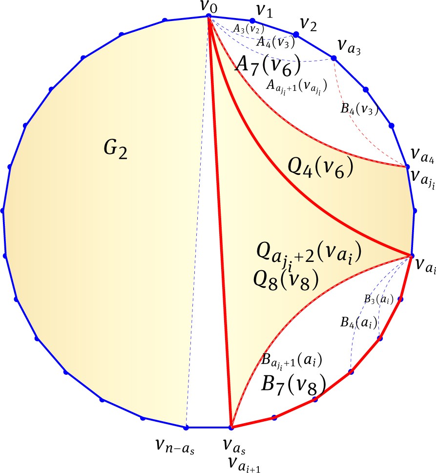
Q_aji+2(a_i) on G₁

We shall construct the triangulation T_G1 of G₁, and then G₂ can be triangulated in a similar way.

(∗) It is important to mention that in the following argument the property a_i+1 − a_i ∈ S_n, for each two consecutive values a_i and a_i+1 in S_n, and 1, 2 ∈ S_n, are basic tools to construct T_G1.

Let a_i, a_i+1 be two consecutive vertices in S_n and a_i+1 − a_i = a_ji ∈ S_n for some a_ji ∈ {1, 2, a₃, …, a_i} (since S_n is a set of ascending values). Let v₀v_aiv_ai+1 … v_ai+1v₀ be a convex (a_ji+2)-gon in G₁ denoted by Q_aji+2(v_ai). Clearly G1=∪i=1s−1Qaji+2(vai). First, we prove Q_aji+2(v_ai) can be triangulated by edges of C(n, S_n) for each i = 1, …, s − 1.

Note that a₁ = 1, a₂ = 2 and a₃ ∈ {3, 4} (otherwise, if a₃ = 5 then a₃ − a₂ = 5 − 2 = 3 ∉ S_n, a contradiction). It is easy to see that Q₃(v₁) ( = v₀v₁v₂v₀) is triangulated by v₀v₁v₂v₀ and when a₃ = 3 we have Q₃(v₂) ( = v₀v₂v₃v₀) is triangulated by v₀v₂v₃v₀, and also when a₃ = 4 we have that Q₄(v₂) ( = v₀v₂v₃v₄v₀) is triangulated by the boundary edges v₀v₂v₃v₄v₀ together with the diagonal edge v₂v₄.

Now we obtain a triangulation for Q_aji+2(v_ai), i = 3, …, s − 1.

Let A_ai+1(v_ai) = v₀v₁ … v_aiv₀, be a convex (a_i+1)-gon in G₁. Clearly, A₃(v₂) ( = v₀v₁v₂v₀) is a triangle that is trivially triangulated by T₁ = v₀v₁v₂v₀. If i = 3, then either a₃ = 3 and A₄(v₃) ( = v₀v₁v₂v₃v₀) is a quadrilateral that is triangulated by T₂ = v₀v₂ ∪ v₀v₁v₂v₃v₀, or a₃ = 4 and A₅(v₄) ( = v₀v₁v₂v₃v₄v₀) is a pentagon triangulated by T₂ = v₀v₂v₄ ∪ v₀v₁v₂v₃v₄v₀.

Let B_aji+1(v_ai) = Q_aji+2(v_ai) − v₀. Then B_aji+1(v_ai) = v_aiv_ai+1 … v_ai+ajiv_ai (since a_i+1 − a_i = a_ji) which is equivalent to the convex polygon v₀v₁ … v_ajiv₀ (by considering a_i = 0). Thus, B_aji+1(v_ai) is equivalent A_aji+1(v_aji).

If i = 3, we have a₄ − a₃ = a_j3 ∈ S_n for some a_j3 ∈ {1, 2, a₃}. Then, B_aj3+1(a₃) ( = v_a3v_a3+1 … v_a4v_a3 = v_a3v_a3+1 … v_a3+aj3v_a3) is equivalent to A_aj3+1(a_j3) ( = v₀v₁ … v_aj3v₀) which is triangulated by T ∈ {T₁, T₂}. Then, B_aj3+1(a₃) can be triangulated by T′ equivalent to T. Hence, T₃ = T′ ∪ v_a3v₀v_a4 is a triangulation of Q_aj3+2(v_a3).

Recursively, if we have i = s − 1 then a_s − a_{s − 1} = a_{js − 1} ∈ S_n for some a_{js − 1} ∈ {1, 2, a₃, …, a_{s − 1}}. Then, B_{ajs − 1+1}(v_{as − 1}) is equivalent to A_{ajs − 1+1}(a_{js − 1}) which is triangulated by T ∈ {T₁, T₂, T₃, …, T_{s − 2}} (depending on the value of a_{js − 1} ∈ {1, 2, a₃, …, a_{s − 1}}). Then, B_{ajs − 1+1}(v_{as − 1}) can be triangulated by T′ equivalent to T. Hence, T_{s − 1} = T′ ∪ v_{as − 1}v₀v_as is a triangulation of Q_{ajs − 1+2}(v_{as − 1}).

Since, G1=∪i=1s−1Qaji+2(vai), then let TG1=∪i=1s−1Ti be the triangulation of G₁. In a similar way we obtain T_G2. Thus, T_n = T_G1 ∪ T_G2 ∪ {v_asv_{n − as}}, where a_s ≠ n − a_s; otherwise {v_asv_{n − as}} = ∅ is a restricted triangulation of G. □

Corollary 2.4

Let n ≥ 4 be a natural number. Suppose G = C(n, S) is a circulant graph. Then G admits a restricted triangulation if one of the following conditions hold.

1. S = {1, 2, a₃, a₄, …, ⌊n2⌋} whereai′s are consecutive odd values.

2. S = {1, 2, a₃, a₄, …, ⌊n2⌋} whereai′are consecutive even values.

Proof

In both cases a₁ = 1, a₂ = 2 and ⌊n2⌋ are in S. Further, for each a_i+1, a_i ∈ S_n, a_i+1 − a_i ∈ {1, 2} ⊆ S_n. Then the circulant graph C(n, S) admits a restricted triangulation by Proposition 2.3. □

Now, we shall define a smallest size circulant graph that admits a restricted triangulation. Before proceeding, we present some ingredients that will be used to prove the main results in this section.

1. When n is even number, then n can be written as n = t.2^r′ for some positive natural number r′ and some positive odd natural number t.

2. Let S_α be a set of jump values obtaining by next algorithm where α = ⌊t3⌋ and β = ⌊t3⌋ with t = n,n is odd ;t,n=t.2r′.

3. Let S₁ = {1, 2, 4, 8, …, c} with c = 2^r where r=0,n is odd ;r′−1,t=1;r′,t≥3.

4. If we have a set B = {b₁, b₂, …, b_k} of positive integers, then define a.B to be {a.b₁, a.b₂, …, a.b_k} where a ≥ 1 is an integer number.

Algorithm (A)

1. If α = 0, then let S_α = {β} and Stop. If α = 1, then let S_α = {1, β} and Stop. If 2 ≤ α ≤ 4, then let S_α = {1, 2, α, β} and Stop. Otherwise, let L = 0 be the number of starting level. Let S(L) = {1, 2, β}, a₀ = α, and let L = L+1.

2. 2- If a₀ is odd and divisible by 3, then let a_{1, L} = a03 and a_{2, L} = 2.a_{1, L}. Otherwise, let a_{1, L} = ⌊ a02⌋ and a_{2, L} = ⌈ a02⌉.

3. Let S(L) = {a_{1, L}, a_{2, L}, a₀}. Let Sα=⋃l=0LS(l).

4. If 3 ∈ {a_{1, L}, a_{2, L}} and each of α and ⌊α2⌋ is odd and not divisible by 3, then do the following:

   1. Let L = 0 be the number of starting level. Let S(L) = {1, 2, 3, α − 3, α, β}, a₀ = α − 3, and let L = L+1.

   2. If a₀ is odd and not divisible by 3, then let a_{1, L} = a_{2, L} = a₀ − 3. If a₀ is odd and divisible by 3, then let a_{1, L} = a03 and a_{2, L} = 2.a_{1, L}. Otherwise, a_{1, L} = a_{2, L} = a02.

   3. Let S(L) = {a_{1, L}, a_{2, L}, a₀}. Let Sα=⋃l=0LS(l).

   4. If a_{1, L} ≤ 3, then arrange S_α to be a set of ascending values and stop. Otherwise, let a₀ = a_{1, L} and L = L+1 and then repeat Step (ii).

5. If a_{1, L} ≤ 4, then arrange S_α to be a set of ascending values and stop. Otherwise, let a₀ = a_{1, L} and L = L+1 and then repeat Step (2).

Note that, S_α that obtained by Algorithm (A) is a set of ascending values 1, 2, a_{i − 1}, a_i, a_i+1, …, α, β.

Lemma 2.5

Suppose S_α = {a₁, a₂, …, α, β} is a set obtained by Algorithm (A). Then 1, 2 ∈ S_α and a_i+1 − a_i ∈ S_αfor each a_i+1, a_i belong to S_α.

Proof

By Algorithm (A) step (1), we get 1, 2 ∈ S_α. Suppose that, a_i, a_i+1 are two consecutive values belonging to S_α.

If a_i+1 = a₀ is an odd and divisible by 3 number, then by Algorithm (A) Step (2), ai=a2,L=2.ai+13. Thus, ai+1−ai=ai+1−2.ai+13=ai+13=ai−1∈Sα (where ai−1=a1,L=ai+13∈Sα).

If 3 ∈ S_α and a_i+1 = a₀ is an odd and not divisible by 3 number, then by Algorithm (A) Step (4), a_i = a_i+1 − 3. Thus, a_i+1 − a_i = 3 ∈ S_α.

Otherwise, by Algorithm (A) Step (2), ai=⌈ai+12⌉(where ⌈ai+12⌉=a2,L∈Sα). Hence, ai+1−ai=ai+1−⌈ai+12⌉=⌊ai+12⌋=ai−1∈Sα (where ai−1=⌊ai+12⌋=a1,L∈Sα). In case when, ⌈ai+12⌉=⌊ai+12⌋=ai+12, then we have ai=ai+12. Thus, ai+1−ai=ai+1−ai+12=ai+12=ai∈Sα.

Theorem 2.6

Let S(n) = S₁ ∪ c.S_α, where n ≥ 4. Then C(n, S(n)) admits a restricted triangulation.

Proof

Suppose that C(n, S(n)) is a circulant graph and let α, β, c and t is defined as above. We shall construct a restricted triangulation T_n of C(n, S(n)).

When n is even and t = 1, S(n) = S₁ (In this case, β = 1 and then S_α = {1} and then c. S_α = {c} and c ∈ S₁). Then let Tn=⋃i=0r{vj2iv(j+1)2i,j=0,1,…,n2i−1}. The circulant graph when n = 8 is depicted in Figure 2.

Fig. 2

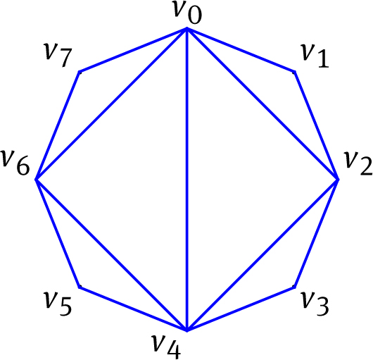
n = 8 = 2³, t = 1, r = r′ − 1 = 2, T₈ = {v_jv_(j+1), j = 0, …, 7} ∪ {v_2jv_2(j+1), j = 0, …, 3} ∪ {v_4jv_4(j+1), j = 0, 1}.

When n is even and t ≥ 3, S(n) = S₁ ∪ c.S_α. In this case, and also when n is odd (which means t = n), we have t-gon which is induced by the vertices v₀, v_c, v_2.c, …, v_{(t − 2).c}, v_{(t − 1).c} (the shaded part in Figure 3).

We shall triangulate this t-gon by T′ which is obtained by one of the following three cases depending on S_α. According to S₁, let T=⋃i=0r{vj2iv(j+1)2i,j=0,1,…,n2i−1} which triangulates unshaded part, between n-gon and t-gon, in Figure 3.

Fig. 3

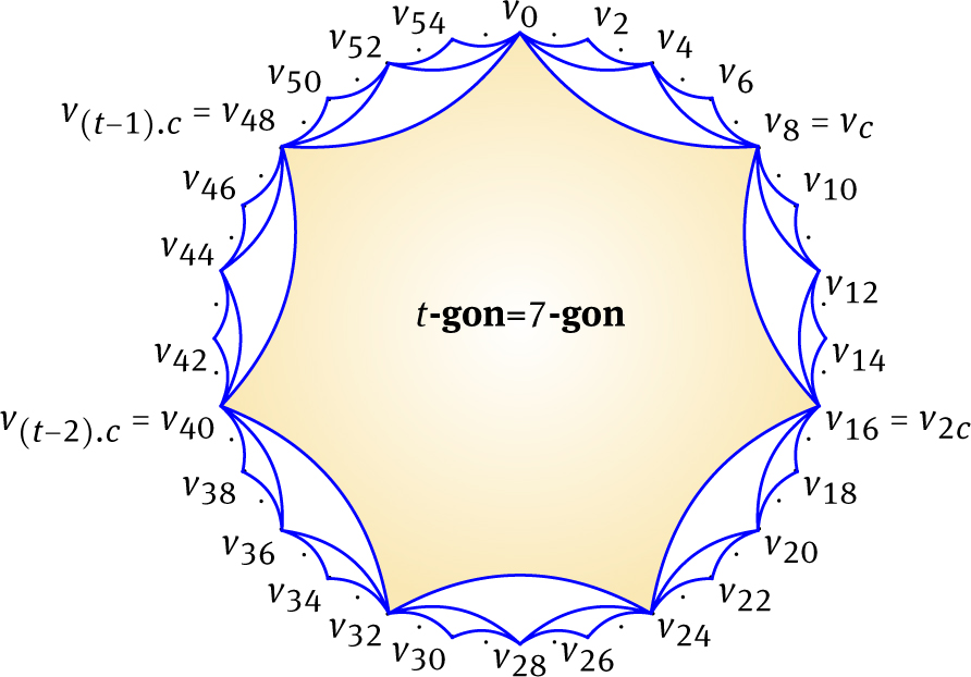
n = 56 = 7.2³, t = 7, r = r′ = 3, T₅₆ = {v_jv_(j+1), j = 0, …, 55} ∪ {v_2jv_2(j+1), j = 0, …, 27} ∪ {v_4jv_4(j+1), j = 0, …, 13} ∪ {v_8jv_8(j+1), j = 0, …, 6}.

Then, let T_n = T ∪ T′ or T_n = T′ be a triangulation to C(n, S(n)) when n is even with t ≥ 3 or when n is odd, respectively.

1. When α = t−23, then t = 2β+α (since β = α+1). Let △ = v₀v_αv_α+βv₀ be a triangle. Then there are three (α + 1)-gons G₁, G₂ and G₃ induced by the vertices v₀, v_c, v_2.c, …, v_α.c; v_(α).c, v_(α+1).c, …, v₂α.c and v_(α+β).c, v_(2α+2).c, …, v_(3α+1).c, respectively. See Figure 4.

   

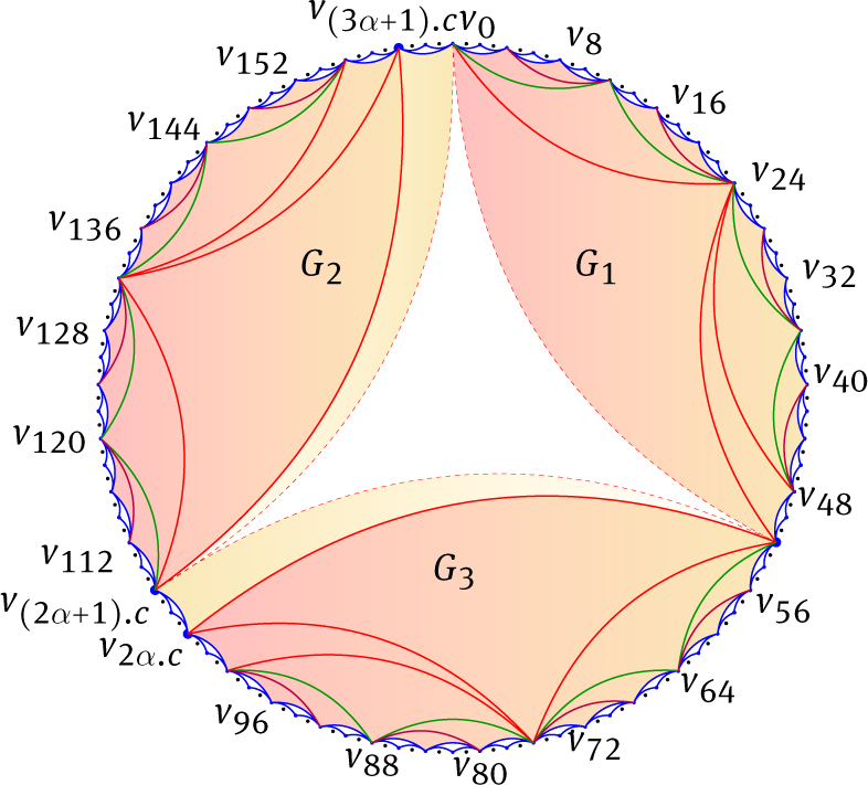   Fig. 4

   n = 164, t = 41, r = 2, α = 13, and β = 14.

2. When α = t−13, then t = 2α+β (since β = α + 1). Let △ = v₀v_αv_2αv₀ be a triangle. Then there are three (α + 1)-gons G₁, G₂ and G₃, induced by the vertices v₀, v_c, v_2.c, …, v_α.c; v_(α).c, v_(α+1).c, …, v₂α.c and v_(2α).c, v_{(2α + 1).c}, …, v_(3α).c, respectively. See Figure 5.

   

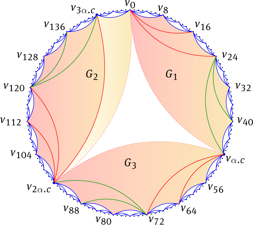   Fig. 5

   n = 152, t = 19, r = 3, α = 6, and β = 7.

3. When α = t3, then t = 3α. There are three (α + 1)-gons G₁, G₂ and G₃ induced by the vertices v₀, v_c, v_2.c, …, v_α.c; v_(α).c, v_(α+1).c, …, v₂α.c and v₂α.c, v_(2α+1).c, …, v_(3α−1).c, v₀, respectively. See Figure 6.

   In each case, G₁, G₂ and G₃ are of the same order. Suppose that R is an r-gon in G_i, for some i ∈ {1, 2, 3} such that V(R) = {v_h, v_h+ai, v_h+a_i+1, …, v_h+ai+1} for some v_h ∈ V(G_i) and two consecutive jump values a_i and a_i+1 in S_α.

   Without loss of generality assume that R is a subgraph of G₁ and h = 0.

   By Lemma 2.5, we have 1, 2 ∈ S_α and a_i+1 − a_i ∈ S_α for each a_i+1, a_i belonging to S_α. Hence, we can use the argument (∗) of Proposition 2.3 to show that R can be triangulated by T_r. Moreover, similar as in the proof of Proposition 2.3 we can consider G₁ as a finite union of such polygons. Then we can assume that T_G1 is a finite union of the restricted triangulation of these polygons.

   Obtain T_G2 (on G₂) and T_G3 (on G₃) by “rotating” the edges of T_G1, see Figures 4, 5 and 6. Let T′ = T_G1 ∪ T_G2 ∪ T_G3 ∪ △ for case (1) and case (2), and let T′ = T_G1 ∪ T_G2 ∪ T_G3 for case (3).

   

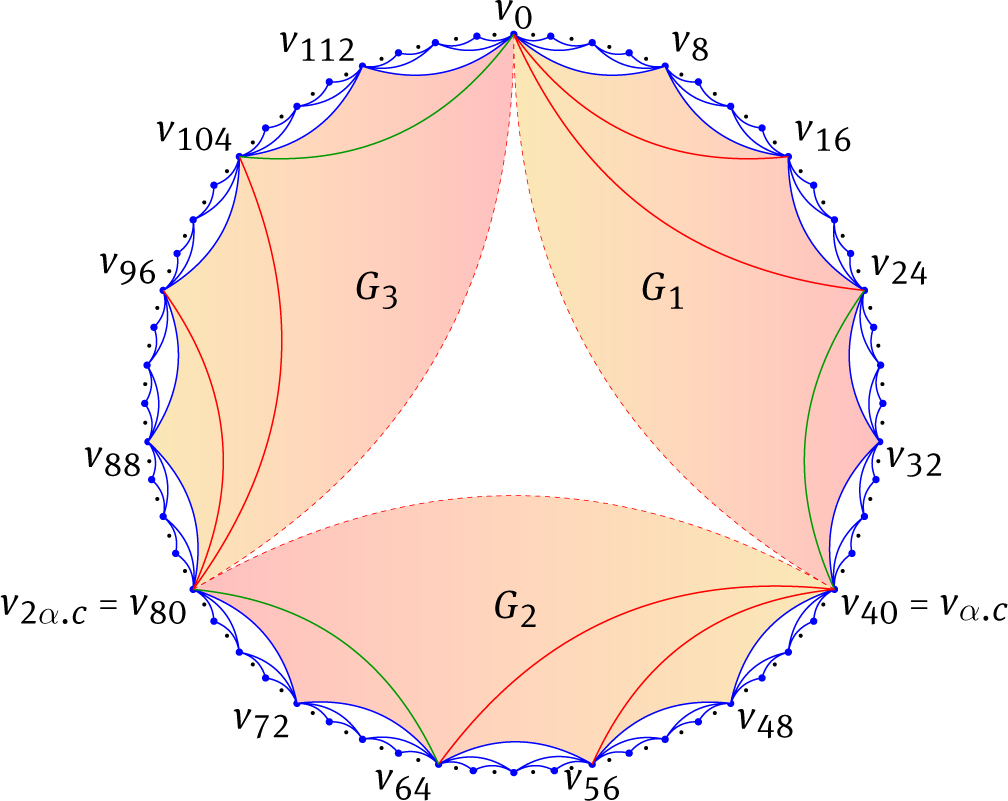   Fig. 6

   n = 120, t = 15, r = 3, and α = 5.

   This completes the proof.

Definition 2.7

Letn ≥ 4 andtbe defined as above, and leta_kbe a natural number such that ⌈t3⌉ ⋅ c ≤ a_k ≤ ⌊n2⌋. Then defineS^*to be a set of ascending natural numbers such that,

1. S^* = {1, 2, a₃, a₄, …, a_k},

2. there is {x, z} ⊂ S^*such thatn = x + y + z wherey ∈ {0, a_i} for somei ∈ {1, …, k},

3. a_i+1 − a_i ∈ S^*for eachi = 1, …, k − 1.

Theorem 2.8

SupposeG = C(n, S) is a circulant graph. Gadmits a restricted triangulation if and only ifScontainsS^*.

Proof

Let G have a restricted triangulation T_n. We shall prove that S contains S^*. By Lemma 2.1, it is enough to prove S^* = D(T_n).

Arrange the spans of D(T_n) to be ascending values.

Since, the circulant graph C(n, D(T_n)) admits T_n, then by Proposition 2.2, we have {1, 2} ⊆ D(T_n).

Let |D(T_n)| = s, then d_s is the maximum span in D(T_n).

(⋆) Let t be defined as before. Suppose that d_s < ⌈t3⌉ ⋅ c. Without loss of generality assume that, c = 1 and d_s = ⌈t3⌉ − 1. Thus, d_s = t−b3 − 1, b ∈ {0, 1, 2} and then 3d_s + b + 3 = t. Let R be a convex r-gon induced by the vertices v_ds, v_2ds, v_3ds, v₃d_s+1, …, v_3ds+b+1, v_{3ds+b +2}, v_t (recall that, v_t = v_3ds+b+3). Suppose that T_r = T_n(R) is a subgraph of T_n that triangulates R and let e be an edge in T_r such that the span of e is the maximum with respect to D(T_r). Then:

1. either e = v_2dsv_t which yields that its span t − 2d_s ∈ D(T_r) ⊂ D(T_n); but t-2d_s > d_s + 1 (by above assumption, t − 2d_s = d_s + b + 3 > d_s + 1), which is a contradiction with maximality of d_s ∈ D(T_n);

2. or, e = v_dsv₃d_s which yields that 3d_s − d_s = 2d_s ∈ D(T_r) ⊂ D(T_n); but 2d_s > d_s, which also contradicts the maximality of d_s ∈ D(T_n).

Hence, R is not triangulated by T_n which is a contradiction with C(n, S) admitting a restricted triangulation T_n. Thus, d_s ≥ ⌈t3⌉ ⋅ c.

Now, in order to check property (ii) of S^* we have to consider two cases:

1. If d_s = n2, then n = 2.d_s. Hence let x = z = d_s and y = 0.

2. If ⌈t3⌉ ⋅ c ≤ d_s ≤ n−12, then T_n contains a triangle △ = v_hv_h+dsv_h+ds+div_h for some d_i ∈ D(T_n) and v_h ∈ V(G). The span of the edge v_h+ds+div_h ∈ E(T_n) is n − (d_s+d_i) ∈ D(T_n) (by definition of the span of edge). Hence let x = d_s, y = d_i and z = n − (d_s+d_i), then n = x + y + z.

   To check the property (iii) of S^*, assume that d_i and d_i+1, i ∈ {1, 2, …, s − 1} are two consecutive spans in D(T_n).

   If d_s = n2, then let T₁ and T₂ be two subgraphs of T_n induced by the vertices v₀, v₁, v₂, …, v_x; v_x, v_x+1, …, v_x+y − 1, v₀ respectively (x = n2). Let R be a polygon induced by the vertices v_j, v_j+d_i, …, v_j+d_i+1 where v_j ∈ V(T_i) and v_jv_j+di and v_vv_j+di+1 are two diagonals in T_i for some i ∈ {1, 2}.

   If ⌈t3⌉ ⋅ c ≤ d_s ≤ n−12, then let T₁, T₂ and T₃ be three subgraphs of T_n induced by the vertices v₀, v₁, v₂, …, v_x, v_x, v_x+1, …, v_x+y, and v_x+y, v_x+y+1, …, v_x+y+z−1, v₀ respectively. Let R be a polygon induced by the vertices v_j, v_j+di, …, v_j+d_i+1 where v_j ∈ V(T_i) and v_jv_j+di and v_jv_j+di+1 are two diagonals in T_i for some i ∈ {1, 2, 3}.

   Assume without loss of generality that v_jv_j+di and v_jv_j+di+1 are two diagonals in T₁. Then, j < j + d_i < j + d_i+1 (by definitions of T₁ and R). It is clear that, v_jv_j+di … v_j+d_i+1v_j ⊂ T₁. Let T_r = T₁(R) be a subgraph of T₁ that triangulates R with the boundary edges v_jv_j+di … v_j+d_i+1v_j of R.

   Suppose that v_j+div_j+di+1 ∉ E(T_r). Then there is d_i < d < d_i+1 such that v_jv_j+d ∈ E(T_r). This implies that, d ∈ D(T_r) ⊂ D(T_n), a contradiction with d_i and d_i+1 are two consecutive spans in D(T_n).

   Hence, v_j+div_j+di+1 ∈ E(T_r) ⊂ E(T_n). Then d_i+1 − d_i ∈ D(T_n).

   Thus, D(T_n) = S^*. This completes the proof of the necessity.

   To show the sufficiency, suppose that S^* ⊆ S. Then, C(n, S^*) is a subgraph of C(n, S).

   Let △ = v₀v_xv_x+yv_x+y+z be a triangle (since, x + y + z = n). Clearly, E(△) ⊂ E(G). Then there are three polygons G₁, G₂ and G₃, induced by the vertices v₀, v₁, v₂, …, v_x; v_x, v_x+1, …, v_x+y and v_x+y, v_x+y+1, …, v_x+y+z respectively, and G₂ = ∅ where y ∈ {0, 1}.

   Suppose that R is an r-gon in G_i, for some i ∈ {1, 2, 3} such that V(R) = {v_h, v_h+ai, v_{h+ai +1}, …, v_h+ai+1} for some v_h ∈ V(G_i) and two consecutive jump values a_i and a_i+1 in S^*.

   Without loss of generality assume that R is a subgraph of G₁ and h = 0.

   Since S^* = {1, 2, a₃, a₄, …, a_k} and satisfies that a_i+1 − a_i ∈ S^* for each i = 1, …, k − 1, then we can use argument (∗) of Proposition 2.3 to show that R can be triangulated by T_r. Consider G₁ as a finite union of such polygons. Then we can assume that T_G1 is a finite union of the restricted triangulation of those polygons.

   Obtain T_G2 (on G₂) and T_G3 (on G₃) in a similar way. Then T_G1 ∪ T_G2 ∪ T_G3 is a triangulation of C(n, S^*). Since C(n, S^*) is a spanning subgraph of G, then T_G1 ∪ T_G2 ∪ T_G3 is a triangulation of G.

   This completes the proof. □

Corollary 2.9

S(n) is S^*.

Proof

By definition of S(n), either S(n) = S₁ (when n is even and t = 1) or S(n) = S_α (when n is odd) or else S(n) = S₁ ∪ c.S_α. By definition of S₁, we have that S₁ is a set of ascending values and contains 1, 2; also S_α is a set of ascending values by Algorithm (A) and contains 1, 2 by Lemma 2.5. Thus S(n) is a set of ascending values containing 1, 2.

Now, let ℓ denote the cardinality of S(n).

When S(n) = S₁, a_ℓ = 2^r = n2. Let x = z = a_ℓ and y = 0 then we have n = x + y + z.

When S(n) = S_α or S(n) = S₁ ∪ c.S_α, we have by definition of β, a_ℓ = ⌈t3⌉ ⋅ c. To get n = x + y + z we have three cases. When α = t−23, β = α + 1 and t = 3.α + 2. Let x = c.α, y = z = c.β (since, n = c.t). When α = t−13, β = α + 1 and t = 3.α + 1. Let x = y = c.α, z = c.β. When α = t3, let x = y = z = c.α (since β = α).

Let a_i and a_i+1 be any two consecutive values in S(n). If a_i, a_i+1 ∈ S₁, then a_i = 2ⁱ and a_i+1 = 2ⁱ⁺¹ and then a_i+1 − a_i = 2ⁱ⁺¹ − 2ⁱ = 2ⁱ ∈ S₁. If a_i = 2^r, then a_i is the last value in S₁ and the first in c.S_α (recall that, c = 2^r) and if a_i, a_i+1 ∈ S_α then by Lemma 2.2, a_i+1 − a_i ∈ S_α. Thus, a_i+1 − a_i ∈ S(n) for each a_i+1, a_i ∈ S(n).

This completes the proof. □

Corollary 2.10

Letn ≥ 4 be a natural number. SupposeG = C(n, S) is a circulant graph. ThenGadmits a restricted triangulation if one of the following conditions hold.

1. Whennis odd, Scontains {2} and all odd valuesa_i ≤ a_swhere ⌈n3⌉ ≤ a_s ≤ ⌊n2⌋.

2. Whennis even, Scontains {1} and all even valuesa_i ≤ a_swhere ⌈t3⌉ ⋅ c ≤ a_s ≤ ⌊n2⌋.

Proof

In both cases a₁ = 1, a₂ = 2 belong to a set of ascending values S, and ⌈t3⌉ ⋅ c ≤ a_s ≤ ⌊n2⌋ (when n is an odd natural number, ⌈t3⌉ ⋅ c = ⌈n3⌉). Further, for each a_i+1, a_i ∈ S, a_i+1 − a_i ∈ {1, 2} ⊂ S.

To show the property (2) of S^* we have to consider two cases.

1. When n is an odd natural number. Let n ≥ 7 (When n = 5, then S = {1,2} and clearly C(5, S) admits a restricted triangulation T₅ = {v₀v₁v₂v₃v₄v₀} ∪ {v₀v₂, v₀v₃}). If ⌈n3⌉ is an odd number, then ⌈n3⌉ = a_i for some i ∈ {3, …, s}. If ⌈n3⌉ is an even number, then ⌈n3⌉ + 1 = a_i for some i ∈ {4, …, s}.

   Whether ⌈n3⌉ is odd or even, we have n − 2a_i is odd and 1 ≤ n − 2a_i ≤ a_i. Then n − 2a_i = a_j for some j ∈ {1, …, i}. Let x = y = a_i, z = a_j. Thus, n = x + y + z.

2. When n is an even natural number, we have r ≥ 1 and then c(≥ 2) is even. Hence, ⌈t3⌉ ⋅ c is even and then ⌈t3⌉ ⋅ c = a_i for some i ∈ {2, …, s}. Now, we have n − 2a_i is even and either n − 2a_i = 0 or 2 ≤ n − 2a_i ≤ a_i. If n − 2a_i = 0, let x = z = a_i, y = 0. If 2 ≤ n − 2a_i ≤ a_i, then n − 2a_i = a_j for some j ∈ {2, …, i} and let x = z = a_i, y = a_j. Thus, n = x + y + z.

   By Theorem 2.8, the circulant graph C(n, S) admitting a restricted triangulation.

Proposition 2.11

([13]). SupposeG = C(n, {a₁, a₂, …, a_k}) andH = C(n, {b₁, b₂, …, b_k}) with {a₁, a₂, …, a_k} = q.{b₁, b₂, …, b_k}, where the multiplication is reduced modulonandgcd(q, n) = 1. ThenGis isomorphic toH.

Example 2.12

Letn = 9 andS(n) = {1, 2, 3}.

WhenS₁ = {2, 3, 4}, then we haveS₁ = {2, 6, 4} = 2.{1, 3, 2} = 2.S(n).

WhenS₂ = {1, 3, 4}, then we haveS₂ = {8, 12, 4} = 4.{2, 3, 1} = 4.S(n).

Corollary 2.13

letG = C(n, S) be a circulant graph. Suppose there is an integerq ≥ 1 withgcd(q, n) = 1 such thatS^* ⊆ q.Sorq.S^* ⊆ Swhere the multiplication is reduced modulon. ThenGhas a configuration that admits a restricted triangulation.

Proof

Suppose that, q ≥ 1 is an integer such that gcd(q, n) = 1 and S^* ⊆ q.S or q.S^* ⊆ S. Then, there is a set S′ ⊂ S such that S^* = q.S′ or q.S^* = S′. Thus, by Proposition 2.11, the subgraph H = C(n, S′) of C(n, S) is isomorphic to C(n, S^*). By Theorem 2.8, H = C(n, S′) admits a restricted triangulation. Thus, G has a configuration that admits a restricted triangulation. This completes the proof. □

Corollary 3.1

LetG = C(n, S) be a circulant graph. ThenK_n − Gadmits a restricted triangulation if one of the following conditions hold.

1. If there isS^*such thatS ∩ S^* = ∅.

2. Scontains all oddi of 𝓝 except {1, ⌊ n/2⌋}.

3. Scontains all eveniof 𝓝 except {2, ⌊ n/2⌋}.

Proof

First, it is well known that K_n − C(n, S) = C(n, 𝓝 − S).

Suppose that S ∩ S^* = ∅. Then, 𝓝 − S contains S^* which yields that the circulant graph C(n, 𝓝 − S) admits the restricted triangulation by Theorem 2.8, and this shows the property (1).

In (2), 𝓝 − S contains all even values of 𝓝 together with {1, ⌊ n/2⌋}. In (3), 𝓝 − S contains all odd values of 𝓝 together with {2, ⌊ n/2⌋}. By Corollary 2.4, C(n, 𝓝 − S) admits the restricted triangulation for both cases.

This completes the proof. □

Definition 3.2

([14]). LetK_nbe a convex complete graph withnvertices. F is said to be potentially triangulable inK_nif there exists a configuration of F inK_nsuch thatK_n − F admits a triangulation.

Corollary 3.3

LetG = C(n, S) be a circulant graph. SupposeS^* ⊆ q.(𝓝 − S) for some an integerq ≥ 1 withgcd(q, n) = 1. ThenGis potentially triangulable inK_n.

Proof

Suppose that, q ≥ 1 is an integer such that gcd(q, n) = 1 and S^* ⊆ q.(𝓝 − S) for some S^*. Then, there is a set S′ ⊂ 𝓝 − S such that S^* = q.S′. Then by Proposition 2.11, the subgraph C(n, S′) of C(n, 𝓝 − S) is isomorphic to C(n, S^*). By Theorem 2.8, C(n, S′) has a configuration that admits a restricted triangulation. Thus, C(n, 𝓝 − S) (= K_n − G) admits a restricted triangulation. This completes the proof. □

Theorem 3.4

C(n, S(n)) is the smallest size circulant graph admitting a restricted triangulation ifn ≥ 4.

Proof

Recall that, S(n) = S₁ ∪ c ⋅ S_α. By Theorem 2.6, C(n, S(n)) admits a restricted triangulation. Hence, we just show that S(n) is the smallest cardinality set for which the conclusion remains true.

Assume that C(n, S) is a circulant graph that admits a restricted triangulation where S = {b₁, b₂, b₃, …, b_s} is a set of ascending jump values to C(n, S).

By Theorem 2.8, S contains S^*. Thus, 1, 2 ∈ S and ⌈t3⌉ ⋅ c ≤ b_s ≤ ⌊n2⌋ and for any i ∈ {1, …, s − 1}, b_i+1 − b_i = b_j ∈ S where j ∈ {1, …, i}.

In case when b_i+1 is even we have, according to S_α (by Algorithm (A) step (2) where b_i+1 = a₀ is even) and S₁ (by definition of S₁), that the difference between the two consecutive values b_i and b_i+1 is always b_i.

If j ∈ {1, …, i − 1}, then the number of values in S(n) is less than the number of values in S. If b_i+1 − b_i = b_i ∈ S, then the number of values in S(n) is equal to the number of values in S. Thus, |S| ≥ |S(n)|.

In case when b_i+1 is odd, then b_j ≠ b_i and there are three cases which are depending only on S_α. (by definition of S₁).

1. b_j ∈ {1, 2}.

   In this case, the difference between the two consecutive values b_i and b_i+1 is at most 2. According to Algorithm (A), the difference between the two consecutive values is at most 2 only when b_i = ⌊bi+22⌋ and b_i+1 = ⌈bi+22⌉ or when b_i = 3 and b_i = 5. Then the number of values in S(n) is equal to or less than the number of values in S. Whereas Step (2) and Step (4) of Algorithm (A) give the difference between any two consecutive values being at least 3, which implies |S| ≥ |S(n)|.

   For instance, take b_i+1 = 13 then b_i ∈ {11, 12}. Take S ∈ {S₁, S₂, S₃, S₄, S₅, S₆} where S₁ = {1, 2, 3, 5, 10, 12, 13}, S₂ = {1, 2, 3, 6, 9, 12, 13}, S₃ = {1, 2, 3, 5, 6, 11, 13}, S₄ = {1, 2, 3, 6, 9, 11, 13}, S₅ = {1, 2, 3, 5, 10, 11, 13}, or S₆ = {1, 2, 3, 4, 7, 9, 11, 13}. Then the cardinality of S is 7. By Algorithm (A) step (2):

   1. either, b_i = 7 and b_i−1 = 6 and then S_α = {1, 2, 3, 6, 7, 13}. Thus, the cardinality of S_α is 6;

   2. or, b_i+2 = 25 and then b_i+1 = 13 and b_i = 12. Then, S_α = {1, 2, 3, 6, 12, 13, 25}. In this case, Take S ∈ {S₁, S₂} where S₁ = {1, 2, 3, 5, 10, 12, 13, 25}, and S₂ = {1, 2, 3, 6, 9, 12, 13, 25}. Note that S is of cardinality 8 while S_α is of cardinality 7.

2. j ∈ {3, …, i − 2}.

   In S_α, this case is satisfied in step (4) of Algorithm (A) (when b_i = a₀ is odd and not divisible by 3). But in this case, Algorithm (A) states b_i to be b_i+1 − 3 which is always even. Then by step (2) when b_i(= a₀) is even we have that b_i−1 = bi2. That is, the difference between the two consecutive values b_i and b_i−1 is always b_i−1 (since b_i = 2b_i−1). While, in S, we have either b_i − b_i−1 = b_i−1 and then |S| = |S(n)| or b_i − b_i−1 = b_k ≠ b_i−1 and then |S| > |S(n)|. Thus, |S| ≥ |S(n)|.

   For instance, take b_i+1 = 23 and S = {1, 2, 3, 6, 8, 9, 17, 23}. By Algorithm (A) we have S_α = {1, 2, 3, 5, 10, 20, 23}. Note that S is of cardinality 8 while S_α is of cardinality 7.

3. j = i − 1.

   If b_i+1 is not divisible by 3, then by Algorithm (A) step (2) we have b_j = b_i−1 = ⌊bi+12⌋ and b_i = ⌈bi+12⌉ (where b_i−1 = b_1,L and b_i = b_2,L), and then the difference between the two consecutive values b_i and b_i−1 is 1. While in S, we have either b_i − b_i−1 = 1 and then |S| = |S(n)| or b_i − b_i−1 = b_k ≠ 1 and then |S| > |S(n)|.

   If b_i+1 is divisible by 3, then in S_α by Algorithm (A) step (2) (where b_i+1 = a₀ is odd and divisible by 3). Then b_i−1 = bi+32 and b_i = 2.b_i−1 (where b_i−1 = a_1,L and b_i = a_2,L). That is, the difference between the two consecutive values b_i and b_i−1 is always b_i−1 itself (since b_i = 2.b_i−1). While in S, either b_i − b_i−1 = b_i−1 and then |S| = |S(n)| or b_i − b_i−1 = b_k for some k ∈ {1, 2, … i − 2} and then |S| > |S(n)|.

   This completes the proof.

Theorem 3.5

LetG = C(n, S) be a circulant graph. ThenK_n − Gadmits no restricted triangulation if |E(G)| > L(n).

Proof

Let |E(G)| > L(n). Then |E(K_n − G)| = (n2)−|E(G)|<(n2)−L(n) = 𝓔_ℓ. Then |𝓝 − S| < 𝓔_ℓ. By Theorem 3.4, C(n, 𝓝 − S) (= K_n − G) admits no restricted triangulation.

References

[1] Lloyd E.L., On triangulations of a set of points in the plane, Proc. of IEEE Symposium on Foundations of Computer Science (FOCS), IEEE,(1977), 228 — 240.10.1109/SFCS.1977.21Search in Google Scholar
[2] Schulz A., The Existence of a Pseudo-triangulation in a given Geometric Graph. Proc. 22nd European Workshop on Computational Geometry, March(2006), Delphi, Greece, 17 – 20.Search in Google Scholar
[3] Černý J., Dvořa′k Z., Jelínek, and J. Ka′ra V., Noncrossing Hamiltonian paths in geometric graphs, Discrete Applied Mathematics, (2007), 155(9), 1096—1105.10.1016/j.dam.2005.12.010Search in Google Scholar
[4] Aichholzer A., Cabello S., Fabila-Monroy R., Flores-Peñaloza D., Hackl T., Huemer C., Hurtado F. and Wood D.R., Edge-removal and non-crossing configurations and geometric graph, Discrete Maths. & Theorectical Comput. Sci., (2010), 12, 75–86.10.46298/dmtcs.525Search in Google Scholar
[5] Imran M., Baig A.Q., Bokhary S.A.U.H., Javaid I., On the metric dimension of circulant graphs, Applied Mathematics Letters, (2012), 25, 320 — 325.10.1016/j.aml.2011.09.008Search in Google Scholar
[6] Basic M., Petkovic M.D., Stevanovic D., Perfect state transfer in integral circulant graphs, Applied Mathematics Letters, (2009), 22, 1117–1121.10.1016/j.aml.2008.11.005Search in Google Scholar
[7] Rose D.J., Tarjan R.E., Lueker G.S., Algorithmic aspects of vertex elimination on graphs, SIAM J. Comput. (1976), 5(2), 266–283.10.1137/0205021Search in Google Scholar
[8] Tarjan R.E., Yannakakis M., Simple linear-time algorithms to test chordality of graphs, test acyclicity of hypergraphs, and selectively reduce acyclic hypergraphs, SIAM J. Comput. (1984), 13(3), 566 – 579.10.1137/0213035Search in Google Scholar
[9] Deshpande A., Garofalakis M.N., Jordan M.I., Efficient stepwise selection in decomposable models, Proc. the Seventeenth conference on Uncertainty in artificial intelligence UAI, August 02 - 05 (2001) Seattle, Washington, 128 –135.Search in Google Scholar
[10] Aurenhammer F., Voronoi diagrams - a survey of fundamental geometric data structure, ACM Computing Surveys, (1991), 23, 345–405.10.1145/116873.116880Search in Google Scholar
[11] Floriani L., Surface representation based on triangular grids, The Visual Computer, (1987), 3, 27 – 50.10.1007/BF02153649Search in Google Scholar
[12] Harary F., Graph Theory, (Addison-Wesley, 1969).10.21236/AD0705364Search in Google Scholar
[13] Lu F., Zhang L., Wang Y., The Pfaffian property of circulant graphs, Discrete Applied Mathematics, (2015), 181, 185 -–192.10.1016/j.dam.2014.09.002Search in Google Scholar
[14] Ali N.A., Gek Chia L., Trao H.M., Kilicman A., Triangulability of Convex Graphs and Convex Skewness, arXiv:1611.09033v1 [math.CO], November (2016).Search in Google Scholar
© 2018 Ali et al., published by De Gruyter
This work is licensed under the Creative Commons Attribution-NonCommercial-NoDerivatives 4.0 License.
Articles in the same Issue
- Regular Articles
- Algebraic proofs for shallow water bi–Hamiltonian systems for three cocycle of the semi-direct product of Kac–Moody and Virasoro Lie algebras
- On a viscous two-fluid channel flow including evaporation
- Generation of pseudo-random numbers with the use of inverse chaotic transformation
- Singular Cauchy problem for the general Euler-Poisson-Darboux equation
- Ternary and n-ary f-distributive structures
- On the fine Simpson moduli spaces of 1-dimensional sheaves supported on plane quartics
- Evaluation of integrals with hypergeometric and logarithmic functions
- Bounded solutions of self-adjoint second order linear difference equations with periodic coeffients
- Oscillation of first order linear differential equations with several non-monotone delays
- Existence and regularity of mild solutions in some interpolation spaces for functional partial differential equations with nonlocal initial conditions
- The log-concavity of the q-derangement numbers of type B
- Generalized state maps and states on pseudo equality algebras
- Monotone subsequence via ultrapower
- Note on group irregularity strength of disconnected graphs
- On the security of the Courtois-Finiasz-Sendrier signature
- A further study on ordered regular equivalence relations in ordered semihypergroups
- On the structure vector field of a real hypersurface in complex quadric
- Rank relations between a {0, 1}-matrix and its complement
- Lie n superderivations and generalized Lie n superderivations of superalgebras
- Time parallelization scheme with an adaptive time step size for solving stiff initial value problems
- Stability problems and numerical integration on the Lie group SO(3) × R3 × R3
- On some fixed point results for (s, p, α)-contractive mappings in b-metric-like spaces and applications to integral equations
- On algebraic characterization of SSC of the Jahangir’s graph 𝓙n,m
- A greedy algorithm for interval greedoids
- On nonlinear evolution equation of second order in Banach spaces
- A primal-dual approach of weak vector equilibrium problems
- On new strong versions of Browder type theorems
- A Geršgorin-type eigenvalue localization set with n parameters for stochastic matrices
- Restriction conditions on PL(7, 2) codes (3 ≤ |𝓖i| ≤ 7)
- Singular integrals with variable kernel and fractional differentiation in homogeneous Morrey-Herz-type Hardy spaces with variable exponents
- Introduction to disoriented knot theory