Multipreconditioned GMRES for simulating stochastic automata networks
-
 ,
,

Abstract
Stochastic Automata Networks (SANs) have a large amount of applications in modelling queueing systems and communication systems. To find the steady state probability distribution of the SANs, it often needs to solve linear systems which involve their generator matrices. However, some classical iterative methods such as the Jacobi and the Gauss-Seidel are inefficient due to the huge size of the generator matrices. In this paper, the multipreconditioned GMRES (MPGMRES) is considered by using two or more preconditioners simultaneously. Meanwhile, a selective version of the MPGMRES is presented to overcome the rapid increase of the storage requirements and make it practical. Numerical results on two models of SANs are reported to illustrate the effectiveness of these proposed methods.
1 Introduction
The use of Stochastic Automata Networks (SANs) is of interest in a wide range of applications, including modeling queueing systems [1, 2, 3], communication systems [4, 5], manufacturing systems and inventory control [6]. The generator matrices of these SANs are block tridiagonal matrices with each block diagonal being a sum of tensor products of matrices. To analyze the system performance of a SAN, it is required to find the steady state probability distribution of the SAN. The solution can be obtained by solving a large linear system involving its generator matrix.
Iterative procedures are often employed to compute the steady state probability distribution of SANs, such as the classical Jacobi, Gauss-Seidel, SOR, SSOR and TSS iterative methods [3, 6, 7, 8]. These methods are simple and easy to implement, but they usually suffer from slow convergence and they do not appear to be practical when the size of the generator matrix is huge [6, 9, 10]. Hence, Krylov subspace methods which use the matrix-vector multiplications as their main arithmetic operations are developed. For instance, the popular Arnoldi/FOM, GMRES, CGS, BiCGSTAB and QMR methods and so on [7, 11, 12, 13, 14, 15, 16, 17, 18]. Based on a small-dimension Krylov subspace, such iterative methods are able to efficiently approximate the steady state probability distribution of SANs [7, 10, 19]. However, they may also suffer from slow convergence, even though lots of numerical experiments indicate that they generally outperform the classical iterative methods, refer, e.g., to [3, 7] for details.
It is well known that preconditioning techniques are necessary to improve the convergence of iterative methods by modifying the eigenvalue distribution of the iteration matrix, while the solution remains unchanged. Preconditioners based on incomplete LU factorizations are possible choices and have been discussed in [3, 7, 20]. A SAN preconditioner (based on the Neumann) series was proposed by Stewart et al. [10]. Numerical experiments show that the SAN preconditioner is expensive and needs more executing time. For taking use of the tensor structure of the generator matrix of a SAN, an approximate inverse preconditioner for the SAN was proposed by Langville and Stewart [19]. It is called the Nearest Kronecker Product (NKP) preconditioner. Numerical tests on some SANs have shown the effectiveness of the NKP preconditioner, however it is not always appropriate for general Markov chains [21]. Taking circulant approximations of the tensor blocks of the generator matrix, circulant preconditioners were constructed for a SAN [2, 4]. These are simple to construct and as since circulant matrices can be easily diagonalized by using the fast Fourier transforms [22]. However, the successful applications of these circulant preconditioners depend on whether the tensor blocks of the generator matrix of a SAN are near-Toeplitz matrices. In fact, different preconditioners have different efficiencies for some model problems. Which one is better and how to develop more efficient preconditioners, especially for very large systems, remains to be done in the future.
In this paper, motivated by the idea of [23], our main contribution is to find the steady state probability distribution of a SAN by employing a variant of GMRES where two or more preconditioners are applied simultaneously, and denote it as multipreconditioned GMRES (MPGMRES). Compared to the standard GMRES, one advantage of the MPGMRES is that it is able to find an approximate solution over a rich search space that has been enlarged by collecting all possible search direction generated by different preconditioners at each iteration. However, its disadvantage is that more memory requirements are required since the search space has an exponential growth at each iteration. Fortunately, a selective version of the MPGMRES (sMPGMRES) is considered by discarding some search directions such that the search space only has a linear growth with the size of problems increasing at each iteration. In fact, the idea to use multiple preconditioners is not new, e.g., Bridson et al. [24] has proposed the multipreconditioned conjugate gradients (MPCG) for symmetric positive definite linear systems. Even though the short-term recurrence of the standard CG does not hold in general, the MPCG is very useful in terms of determining what the most effective preconditioner is by executing a few iterations of the MPCG. On the other hand, for linear systems with a nonsymmetric coefficient matrix, a combined preconditioning strategy has been analyzed in [25] and shows that an optimal linear combination of two preconditioners could obtain the good numerical performance.
The rest of this paper is organized as follows. In Section 2, a brief introduction of two models of SANs is given. The derivation of the MPGMRE and its selective version are discussed in Section 3. In Section 4, numerical experiments on two SANs are employed to illustrate the effectiveness of these methods. Finally, some conclusions are given in Section 5.
2 Two models of SANs
To introduce certain terminologies and notations of SANs, two models will be described in this section; a two-queue overflow network and another one is a telecommunication system.
2.1 A two-queue overflow network
The early research on the two-queue overflow network can be found in [2, 26]. This network consists of two independent queues with the number of servers and waiting spaces being si and li – si – 1 (i = 1, 2) respectively, where li is the total number of customers in the queue i. For queue i, i = 1, 2, let λi be the arrival rate of customers, and let μi be the service rate of the servers, then the state space of the queueing system can be represented by the elements in the following set:
where i represents the state that there are i customers in the queue 1, and j represents the state that there are j customers in the queue 2. Thus it is a two-dimensional queueing system.
Generally speaking, the queueing discipline is First-come-first-served. When a customer arrives and finds all the serves are busy, the customer has two choices: one is to wait in the queue, provided that there is still a waiting space available, another is to leave the system. But for now we allow the overflow of customers from queue 2 to queue 1 whenever it is full and queue 1 is not, see Fig. 1. The generator matrix can be shown to be the following l1l2 × l1l2 matrix in the tensor product form
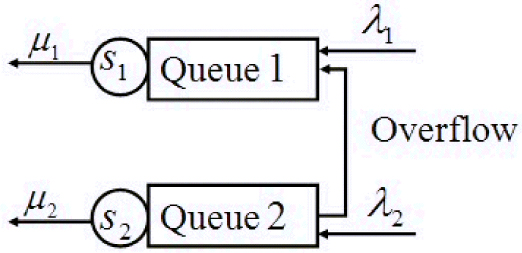
The two-queue overflow network.
where
and Ili is the identity matrix of size li, i = 1, 2, and el2 is the unit vector (0, …, 0, 1)T, see [2, 26] for instance. Let n = l1l2, then the steady state probability distribution vector p = (p1, p2, …, pn)T is the solution of the linear system Ap = 0 with constraints
According to the properties of the tensor product [9, 10, 27], the matrix R ⊗
2.2 A telecommunication system
Here an (MMPP/M/s/s+m) network arising in telecommunication systems is considered. It is known that the Markov Modulated Poisson Process (MMPP) is a generalization of the Poisson process and is often regarded as the input model of telecommunication system [4, 5]. To construct the (MMPP/M/s/s+m) network, first define the system parameters as follows:
1/λ, the mean arrival time of the exogenously originating calls of the main queue,
1/μ, the mean service time of each server of the main queue,
s, the number of servers in the main queue,
l–s–1, the number of waiting spaces in the main queue,
q, the number of overflow,
(Qj, Λj), 1 ≤ j ≤ q, the parameters of the MMPP’s modeling overflow parcels, where
Here σj1, σj2 and λj, 1 ≤ j ≤ q, are positive MMPP parameters.
The input of the main queue comes from the superposition of several independent MMPPs, which is still an MMPP and is parameterized by two 2q × 2q matrices (Q, Ω). Here
and Ω = Λ + λI2q, where I2 and I2q are the 2 × 2 and 2q × 2q identity matrices, respectively.
Now the (MMPP/M/s/l) network can be regarded as a Markov process on the state space
where the number i corresponds to the number of calls at the destination, and the number j corresponds to the state of the Markov process with generator matrix Q. Hence, it is a two-dimensional queueing system, and the generator matrix can be shown to be the following l2q × l2q tridiagonal block matrix:
It can be rewritten as in the tensor product form,
where matrices B and R has the same form as Qi and R in (2) and (3), respectively. Let n = l2q, then steady state probability distribution vector p = (p1, p2, …, pn)T is the solution of the linear system Ap = 0 with the same constraints as (4).
Similarly, the matrix A in (5) is irreducible, has zero column sums, positive diagonal elements and nonpositive off-diagonal elements. According to the famous Perron-Frobenius theory, the matrix A has a one-dimensional null space with a positive null vector [28, 29]. Hence, the steady state probability distribution vector p exists.
Remark 2.1
To solve the linear systemAp = 0 efficiently, it is necessary to make certain modifications to the matrixAsine it is singular. One possible way to obtain the steady state probability distribution vectorpis to normalize the solutionxof the following nonsingular linear system:
whereb = (0, …, 0, 1)Tis an n × 1 vector, Iis as n × nidentity matrix, andϵ > 0 can be chosen as small as possible. The matrix 𝓐 is nonsingular because it is irreducible strictly diagonally dominant. The linear system (6) can be solved by GMRES. It is clear that solving the linear system (6) may induce a small error of O(ϵ), but fortunately Ching et al. have proved that the 2-norm of the error induced by the regularization tends to zero [2, 4].
3 Multipreconditioned GMRES
This section will give a brief description of the preconditioned GMRES, and then discuss the GMRES with multiple preconditioners (MPGMRES). At last, to decrease the computing cost of the MPGMRES, a selective version of the MPGMRES is considered.
3.1 Preconditioned GMRES
GMRES is often used to solve the non-symmetric linear system (6). Given an initial vector x0, then the corresponding initial residual is r0 = b – 𝓐x0, and the Krylov subspace is:
An orthonormal basis for the Krylov subspace 𝓚m(𝓐, r0) can be computed by the modified Gram-Schmidt orthogonalization procedure with the first vector being r0/∥r0∥2. This generates a useful relation:
where Vm ∈ 𝓡n×m and Vm+1 ∈ 𝓡n×(m+1) has orthonormal columns, and H͠m ∈ 𝓡(m+1)×m is an upper Hessenberg matrix. Thus at the k-th step, an approximate solution of (6) is computed as:
where ym =
The preconditioning technique is a key ingredient for the successful applications of GMRES. Let M be a preconditioner, then for the linear system (6), the right preconditioned GMRES is considered in Algorithm 1, refer to Ref. [7].
| Algorithm 1 The right preconditioned GMRES | |
|---|---|
| 1: | Give an initial guess x0, and compute r0 = b – 𝓐x0, β = ∥r0∥2, v1 = r0/β. |
| 2: | forj = 1, …, mdo |
| 3: | Compute w = 𝓐M–1vj. |
| 4: | fori = 1, …, jdo |
| 5: | hi,j = (w, vi) = |
| 6: | w = w – hi,jvi. |
| 7: | end for |
| 8: | Compute hj+1,j = ∥w∥2 and vj+1 = w/hj+1,j. |
| 9: | end for |
| 10: | Let Vm = (v1, …, vm), H͠m = {hij}, 1 ≤ i ≤ j + 1, 1 ≤ j ≤ m. |
| 11: | Compute ym = |
| 12: | If satisfied stop, else set x0 = xm and go to step 1. |
In line 11 of Algorithm 1, the approximate solution xm is expressed as a linear combination of the preconditioned vectors zi = M–1vi, i = 1, 2, …, m, where the preconditioner M is fixed, i.e., it does not change from step to step. Now suppose that the preconditioner is able to change at every step:
Then the approximate solution is computed by xm = x0 + Zmym, where Zm = (z1, …, zm). Such kind of GMRES is called Flexible GMRES (FGMRES) since different preconditioners are allowed to be used at each iteration [30].
3.2 Multiple preconditioned GMRES
Based on the idea of using different preconditioners in the FGMRES, the multipreconditioned GMRES with two or more preconditioners being applied simultaneously was proposed by Greif et. al [23]. Assume there are k preconditioners, i.e., M1, …, Mk, k ≥ 2, then at the beginning, for the initial residual r0, we have v1 = r0/∥r0∥2 and
such that the first iteration is computed by x1 = x0 + Z1y1, where the vector y1 ∈ 𝓡k is chosen to minimize ∥b – 𝓐x1∥2. From (9), it is easy to see that using all preconditioners simultaneously has enlarged the space where the solution is sought. Similar to Algorithm 1, the multipreconditioned GMRES algorithm (i.e., Algorithm 2) is given as follows.
| Algorithm 2 Multipreconditioned GMRES (MPGMRES) | |
|---|---|
| 1: | Give an initial guess x0, and compute r0 = b – 𝓐x0, β = ∥r0∥2, V1 = r0/β. |
| 2: | Compute the research directions Z1 =
|
| 3: | forj = 1, …, mdo |
| 4: | W = 𝓐Zj. |
| 5: | fori = 1,…,jdo |
| 6: | Hi,j = (W, Vi) =
|
| 7: | W = W – ViHi,j. |
| 8: | end for |
| 9: | W = Vj+1Hj+1,j. (QR factorization) |
| 10: | Compute yj =
|
| 11: | If satisfied stop, otherwise continue; |
| 12: | Zj+1 =
|
| 13: | end for |
| 14: | If unsatisfied, set x0 = xm and go to step 1. |
Comparing with Algorithm 1, the search space increases at each iteration, and the relation in the equation (7) has been replaced by:
where
and
in which the matrices Vj+1 and Hj+1,j (1 ≤ j ≤ m) are computed by QR factorization in the line 8 of Algorithm 2. Note that matrices Zj and Vj+1 have kj columns, j = 1, …, m. Thus the matrix V͠m+1 has:
columns, the matrix Z͠m has θm – 1 = (km+1 – k)/(k – 1) columns, and the size of the upper hessenberg matrix H͠m is θm × (θm – 1).
Let 𝓟m–1 = 𝓟m–1(X1, …, Xk) be the space of all possible polynomials of matrices in k variables of at most degree m – 1, then at the j-th step of the MPGMRES, the approximate solution can be represented by:
where
where
and
which implies that, in the matrix polynomial
Theorem 3.1
Letr0be the initial residual of the linear system (6), andrjbe the residual at thej-th step of the MPGMRES withkpreconditionersM1, …, Mk. Then it has:
Therefore, it is important to find an optimal combination of all the different preconditioners as they are used simultaneously at each iteration [23, 24, 25]. This problem still requires further research.
3.3 Selective MPGMRES and computing cost
The idea of the MPGMRES is to enlarge the Krylov subspace over which the GMRES minimizes the residual norm by using two or more preconditioners simultaneously at each iteration. From (14), it can be seen that the reason why the search space is so rich is that it not only has the polynomials of higher order of the variables Xi, but it also has many mixed terms [23]. For instance, when k = 2, the entire space of the matrix polynomials is
It is natural to think of reducing the dimension of the entire space. Specially, for the case when 𝓐 = M1 + M2, the following result has been proved [23].
Theorem 3.2
If the variablesX1, X2satisfy the condition thatX1X2 = X2X1 = X1 + X2, then
The mixed terms have been eliminated, which indicates that the dimension of the entire search space has been reduced successfully. Hence, it is a possible choice to construct an approximate search space by discarding some search directions at each iteration. The computing cost of the MPGMRES will then be decreased.
Several different strategies can be applied to obtain the approximate search space at each iteration, see [23, 31]. In this paper, a one simple method shown in [23], where line 11 of Algorithm 2 has been replaced by
i.e., the preconditioner M1 is used in the first column of Vj+1, M2 is used in the second column of Vj+1, and so on. This is called selective MPGMRES (sMPGMRES). Correspondingly, the column of the matrix Zj, j = 1, …, m, remains k rather than kj. For comparisons, at the j-th iteration, the computing cost of the MPGMRES and sMPGMRES is listed as follows [23].
Table 1, it can be seen that the computing cost of the MPGMRES has an exponential growth, while that of the sMPGMRES only grows linearly.
Comparisons of computing cost.
| matrix-vector products | inner products | |
|---|---|---|
| MPGMRES | kj |
|
| sMPGMRES | k |
|
4 Numerical experiments
In this section, Algorithms 1-2 are tested and the variant (sMPGMRES) introduced in this paper on two models of SANs. One example is from queueing systems, the other from telecommunication systems. In particular, we compare the numerical performance of the MPGMRES, sMPGMRES, standard right preconditioned GMRES and unpreconditioned GMRES (with restart being 10) in terms of the total computing time and iteration steps. For convenience, GMRES(M) is used to denote the right preconditioned GMRES method with the preconditioner M in this section. Convergence histories are shown in figures with the number of iterations on the horizontal axis, and Relres (defined as log10 of the relative residual 2-norms, i.e., log10(∥rj∥2/∥r0∥2)) on the vertical axis. All experiments are carried out with a serial MATLAB implementation of the code, in which parts of the MATLAB code are from https://github.com/tyronerees/krylov_solvers/tree/master/mpgmres.
Throughout our numerical experiments, the stopping criteria is set as ∥rj∥2/∥r0∥2 ≤ 10–6, where rj is the current residual and r0 is the initial residual. The initial vector for all methods is chosen to be x0 = (0, …, 0, 1)T. The parameter ϵ in the equation (6) is given as ϵ = 0.5, other numbers can also be used if they can make the coefficient matrix 𝓐 be nonsingular.
Example 4.1
The two-queue overflow network [2, 26]. This test problem was introduced in Section 2.1. The corresponding matrices can be found in the equations (1), (2) and (3). Here set λ1 = μ1 = s1 = 1, and λ2 = μ2 = s2 = 2. The size of the matrix 𝓐 isn = l1l2. To find the steady state probability distribution, different ways can be applied to construct different preconditioners in order to solve the linear system (6).
Case one: Consider the incomplete LU factorization with “droptol = 0.001” for the coefficient matrix 𝓐, i.e., 𝓐 = LU + E, whereLis an unit lower triangular matrix andUis an upper triangular matrix. Hence the matricesLandUare used as two preconditioners for the GMRES. Numerical results for this case are shown in Table 2.
The number of iterations and computing time in seconds (in brackets) for Example 4.1 when L and U are used as preconditioners. The last column Ratio is defined as (computing time of sMPGMRES)/(computing time of GMRES).
| l 1 | l 2 | MPGMRES | sMPGMRES | GMRES | Ratio |
|---|---|---|---|---|---|
| 128 | 64 | 7 (8.8789) | 13 (0.0619) | 72 (0.0872) | 0.71 |
| 128 | 128 | 7 (24.1441) | 12 (0.1136) | 71 (0.1353) | 0.84 |
| 256 | 256 | 7 (106.1802) | 12 (0.5188) | 71 (0.7215) | 0.72 |
| 512 | 256 | 7 (328.3111) | 13 (1.9379) | 71 (2.6381) | 0.73 |
| 512 | 512 | 7 (634.2202) | 12 (3.5193) | 71 (6.7186) | 0.52 |
Table 2 shows that the iteration counts of the MPGMRES and sMPGMRES with two preconditionersLandUbeing used simultaneously are less than those of the unpreconditioned GMRES. In particular, MPGMRES gives the best iteration steps, even though its computing time is the worst. However, it can be seen that the computing time of the sMPGMRES is superior to that of the unpreconditioned GMRES. The last column in Table 2 further confirms the fast convergence of the sMPGMRES. For instance, whenl1 = 512, l2 = 512, the computing time needed by the sMPGMRES is almost only half of that needed by the unpreconditioned GMRES. Moreover, Fig. 2 (left) plots their convergent histories whenl1 = 128 andl2 = 128.
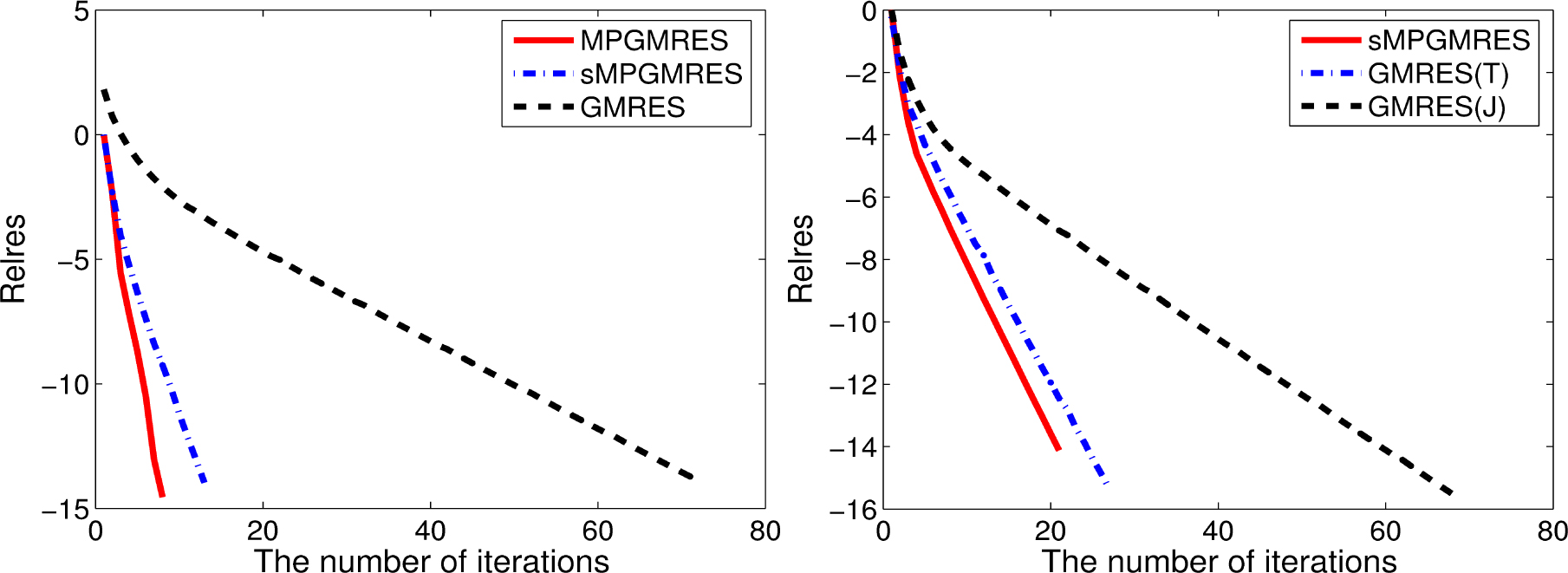
Convergent histories of the MPGMRES, sMPGMRES and unpreconditioned GMRES for Example 4.1 when l1 = 128 and l2 = 128 (left). Convergence histories of the sMPGMRES, GMRES(T) and GMRES(J) for Example 4.1 when l1 = 512 and l2 = 512 (right).
Case two: LetDandTbe the diagonal and tridiagonal matrices of the matrix 𝓐, respectively. Then, correspondingly, the matricesJ(equals to D) andTare considered as the Jacobi preconditioner and the tridiagonal preconditioner for the GMRES. Numerical results for this case are listed in Table 3.
The number of iterations and computing time in seconds (in brackets) for Example 4.1 when J and T are used as preconditioners. Ratio1 and Ratio2 are defined as (computing time of sMPGMRES)/(computing time of GMRES(T)) and (computing time of sMPGMRES)/(computing time of GMRES(J)), respectively.
| l 1 | l 2 | sMPGMRES | GMRE(T) | GMRE(J) | Ratio1 | Ratio2 |
|---|---|---|---|---|---|---|
| 128 | 64 | 20 (0.1256) | 26 (0.0581) | 68 (0.0738) | 2.16 | 1.70 |
| 128 | 128 | 20 (0.2043) | 26 (0.1102) | 67 (0.1146) | 1.85 | 1.78 |
| 256 | 256 | 20 (0.5576) | 26 (0.5593) | 67 (0.6435) | 1.00 | 0.87 |
| 512 | 256 | 20 (0.9771) | 26 (1.5498) | 68 (2.7222) | 0.63 | 0.35 |
| 512 | 512 | 20 (1.9698) | 26 (3.7703) | 67 (6.6672) | 0.52 | 0.30 |
From Table 3, it can see that the number of iterations required by the sMPGMRES is the best. In terms of the computing time, it is clear to find that the sMPGMRES is superior to the GMRES(T) and GMRES(J) when the size of this test problem becomes larger. While the sMPGMRES needs more computing time than the GMRES(T) and GMRES(J) when the size of this test problem is small. The last two columns of Table 3 illustrate the performance of the sMPGMRES with the size of the test problem increasing. Hence, it shows that, by discarding some search direction at each iteration, using different preconditioners for the GMRES simultaneously can be more effective than using a single preconditioner at each step. Fig. 2 (right) shows their convergent curves whenl1 = 512 andl2 = 512.
Example 4.2
The telecommunication system [4, 5]. This example has been introduced in Section 2.2. The corresponding matrices can be found in the equations (2), (3) and (5). Here we set λ = μ = s = 2, q = 4, σj2 = 1/3 and λj = 1/q, j = 1, …, q. The size of the coefficient matrix 𝓐 isn = l2q. For finding the steady state probability distribution, similar ways to Example 4.1 have been used to construct different preconditioners.
Case one: Using the same incomplete LU factorization as given above for the coefficient matrix 𝓐 generated by (6). Then again, the matricesLandUare used as two preconditioners for the GMRES. The corresponding numerical results for this case are presented in Table 4.
The number of iterations and computing time in seconds (in brackets) for Example 4.2, when L and U are used as preconditioners.
| l | MPGMRES | sMPGMRES | GMRES(L) | GMRES(U) |
|---|---|---|---|---|
| 512 | 5 (0.5675) | 10 (0.0677) | 33 (0.0545) | 15 (0.0308) |
| 1024 | 5 (1.9263) | 10 (0.1765) | 33 (0.1366) | 15 (0.0752) |
| 2048 | 5 (2.0571) | 10 (0.2922) | 33 (0.7859) | 15 (0.2084) |
| 4096 | 5 (2.2701) | 10 (0.4457) | 33 (3.3516) | 15 (0.3071) |
| 8192 | 5 (2.5883) | 10 (0.6451) | 33 (9.0279) | 15 (0.7694) |
| 16384 | 5 (3.2082) | 10 (0.9496) | 33 (19.7403) | 15 (1.5723) |
As seen from Table 4, in the sense of iteration counts, the MPGMRES and sMPGMRES with two preconditioners being applied simultaneously are superior to the GMRES with single preconditioner. And in terms of the computing time, the MPGMRES and sMPGMRES cost more than the GMRES(L) and GMRES(U) when the size of this test problem is small. The reason may be that the dimension of the Krylov subspaces has an increase when two preconditioners are used simultaneously. However, when the size of the test problem increases, it is not difficult to see that the sMPGMRES has given the best results, e.g., whenl = 16384, the computing time of the GMRES(L) and GMRES(U) have been reduced by 95% and 40%, respectively. Fig. 3 (left) shows their convergent histories whenl = 8192. Note that the computing time of the sMPGMRES is always less than that of the MPGMRES, which indicates that appropriately discarding some search direction from MPGMRES can lead to fast convergence, even though the iteration steps have a little increase. Therefore, the GMRES with multiple preconditioners is a competitive and robust choice for the large test problem.
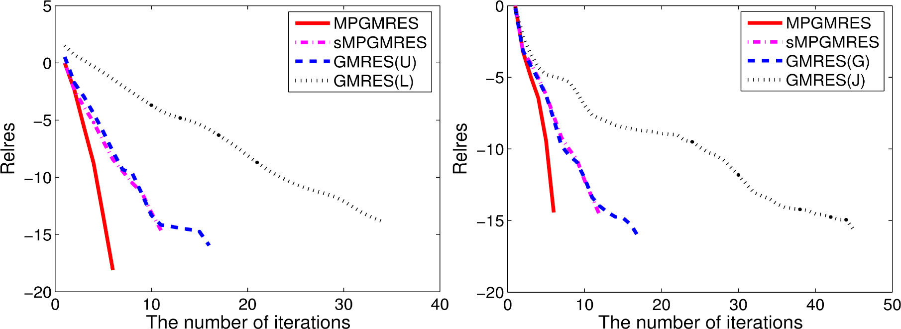
Convergent histories of the MPGMRES, sMPGMRES, GMRES(L) and GMRES(U) for Example 4.2 when l = 8192 (left). Convergent histories of the MPGMRES, sMPGMRES, GMRES(G) and GMRES(J) for Example 4.2 when l = 8192 (right).
Case two: Let us split the coefficient matrix 𝓐 as 𝓐 = D – E – F, whereDis the diagonal of 𝓐, –E and –F are the strict lower triangular and strict upper triangular of 𝓐, respectively. There is also the Gauss-Seidel (GS) preconditonerG = D – F and the Jacobi preconditionerJ (equals toD). Numerical results for this case are supplied in Table 5.
The number of iterations and computing time in seconds (in brackets) for Example 4.2, when G and J are used as preconditioners.
| l | MPGMRES | sMPGMRES | GMRES(G) | GMRES(J) |
|---|---|---|---|---|
| 512 | 5 (1.0332) | 11 (0.2172) | 16 (0.0588) | 44 (0.0502) |
| 1024 | 5 (1.6542) | 11 (0.3605) | 16 (0.1154) | 44 (0.0897) |
| 2048 | 5 (1.7015) | 11 (0.3905) | 16 (0.1994) | 44 (0.2741) |
| 4096 | 5 (1.8292) | 11 (0.4545) | 16 (0.4262) | 44 (0.5751) |
| 8192 | 5 (2.1279) | 11 (0.6181) | 16 (0.8906) | 44 (2.1283) |
| 16384 | 5 (2.7101) | 11 (0.9103) | 16 (2.0081) | 44 (4.7786) |
Again, from Table 5, it is shown that the iteration counts of the MPGMRES and sMPGMRES are less than those of the GMRES(G) and GMRES(J). With the increase of the size of this test problem, the computing time of the MPGMRES and sMPGMRES are superior to that of the GMRES(J), although the computing time of the MPGMRES is inferior to that of the GMRES(G). In particular, the sMPGMRES shows the best results, e.g., whenl = 16384, the computing time of the GMRES(G) and GMRES(J)are reduced by 55% and 81%, respectively. Furthermore, Fig. 3 (right) plots their convergent histories whenl = 8192, withGandJbeing two preconditioners.
Case three: Three preconditioners are applied to the GMRES. Observe the equation (5), it can be seen that the matrixAconsists of three parts. According to the properties of the tensor product [9, 10, 27], the last part of the matrixA, i.e., R ⊗ Ω, is a lower triangular matrix. Since the last diagonal element of the matrixRis zero as shown in the form of (3), the tensor productR ⊗ Ωis a singular matrix. To modify its singularity, let the last diagonal element ofRbe equal to λ, and denote the new matrix asR͠. Then letM3 = R͠ ⊗ Ω. It is nonsingular. On the other hand, using the tensor construct of the matrixAgiven in (5), we letM1andM2be the lower triangular matrices of the tensor productIl ⊗ QandB ⊗ I2q, respectively. Then three preconditionersM1, M2andM3for the linear system (6) are considered for the GMRES. Numerical results for this case are provided in Table 6.
The number of iterations and computing time in seconds (in brackets) for Example 4.2, when M1, M2 and M3 are used as preconditioners.
| l | MPGMRES | sMPGMRES | GMRES(M1) | GMRE(M2) | GMRES(M3) |
|---|---|---|---|---|---|
| 512 | 20 (3.6583) | 23 (0.1967) | 38 (0.0451) | 37 (0.0916) | 194 (0.2613) |
| 1024 | 20 (4.4979) | 23 (0.2336) | 38 (0.0919) | 37 (0.2168) | 336 (0.7794) |
| 2048 | 20 (5.9025) | 23 (2.3188) | 38 (0.2335) | 37 (0.3816) | 595 (4.0581) |
| 4096 | 20 (8.2599) | 23 (0.4523) | 38 (0.4792) | 37 (0.6017) | 1025 (14.2911) |
| 8192 | 20 (11.6451) | 23 (0.9709) | 38 (1.7371) | 37 (1.7914) | 2080 (104.7501) |
| 16384 | 20 (15.7614) | 23 (1.8284) | 38 (4.2532) | 37 (4.2274) | 4120 (493.6202) |
As seen from Table 6, it finds that the MPGMRES has shown the best iteration steps. In addition, the number of iterations of the sMPGMRES is also less than those of the GMRES(M1), GMRES(M2) and GMRES(M3). From the last column of Table 6, it also observes that the preconditionerM3is not effective since its iteration counts have a large change and the computing time has a dramatic increase with the size of this test problem increasing. However, the preconditionerM3does not affect the stability of the MPGMRES and sMPGMRES, i.e., their iteration steps have no changes and their computing time are acceptable. In particular, for large test problem, the sMPGMRES gives the best computing time, e.g., whenl = 16384, the computing time of the GMRES(M1), GMRES(M2) and GMRES(M3) are reduced by 57%, 57% and 99%, respectively. Hence, the acceptable efficiency of the GMRES with multiple preconditioners is illustrated again.
5 Conclusions
In the current study, the main contribution is to consider the MPGMRES for computing the steady state probability distribution of SANs. The idea of the MPGMRES is to enlarge the Krylov subspace over which the GMRES minimizes the residual norm by using two or more preconditioners simultaneously at each iteration. Since the dimension of the search space has an exponential growth at each iteration, a practical sMPGMRES is given by discarding some search directions at each iteration, such that the dimension of the search space only has a linear growth with the problem size. Numerical experiments on two models of SANs have illustrated that the MPGMRES is more effective than the GMRES with a single preconditioner in reducing the number of iterations. Moreover, for large test problems, the computing time of the sMPGMRES is the best.
Here it is worth noting that only the MPGMRES has been tested on two models of SANs. In fact, there are several other models of SANs, e.g., manufacturing systems [6, 32], node mobility in wireless networks [33] and FTS projects [34]. Hence, it would be interesting to extend method to these models in the future.
Acknowledgement
The authors would like to thank the editor Dr. Agnieszka Bednarczyk-Dragthe and anonymous referees for their constructive comments and helpful suggestions in revising the paper. This research is supported by the National Natural Science Foundation of China (Nos. 11501085 and 61772003) and the Fundamental Research Funds for the Central Universities (No. JBK1809003).
References
[1] Buchholz P., A class of hierarchical queueing networks and their analysis, Queueing Sys., 1994, 15, 59-80.10.1007/BF01189232Search in Google Scholar
[2] Chan R.H., Ching W.K., Circulant preconditioners for stochastic automata networks, Numer. Math., 2000, 87, 35-57.10.1007/s002110000173Search in Google Scholar
[3] Stewart W.J., Probability, Markov Chains, Queues, and Simulation, 2009, Princeton University Press, Princeton, NJ.10.1515/9781400832811Search in Google Scholar
[4] Ching W.K., Chan R.H., Zhou X.Y., Circulant preconditioners for Markov-modulated Poisson process and their applications to manufacturing systems, SIAM J. Matrix Anal. Appl., 1997, 18, 464-481.10.1137/S0895479895293442Search in Google Scholar
[5] Meier-Hellstern K., The analysis of a queue arising in overflow models, IEEE Trans. Commun., 1989, 37, 367-372.10.1109/26.20117Search in Google Scholar
[6] Buzacott J., Shanthikumar J., Stochastic Models of Manufacturing Systems, 1993, Prentice-Hall International Editions, Upper Saddle River, NJ.Search in Google Scholar
[7] Saad Y., Iterative Methods for Sparse Linear Systems, 2nd ed., 2003, SIAM, Philadelphia, PA.10.1137/1.9780898718003Search in Google Scholar
[8] Wen C., Huang T.-Z., Wang C., Triangular and skew-symmetric splitting method for numerical solutions of Markov chains, Comput. Math. Appl., 2011, 62, 4039-4048.10.1016/j.camwa.2011.09.041Search in Google Scholar
[9] Langville A.N., Stewart W.J., The Kronecker product and stochastic automata networks, J. Comput. Appl. Math., 2004, 167, 429-447.10.1016/j.cam.2003.10.010Search in Google Scholar
[10] Stewart W.J., Atif K., Plateau B., The numerical solution of stochastic automata networks, Eur. J. Oper. Res., 1995, 86, 503-525.10.1016/0377-2217(94)00075-NSearch in Google Scholar
[11] Saad Y., Schultz M.H., GMRES: A generalized minimal residual algorithm for solving nonsymmetric linear systems, SIAM J. Sci. Stat. Comput., 1986, 7, 856-896.10.1137/0907058Search in Google Scholar
[12] Zhang H.-F., Huang T.-Z., Wen C., Shen Z.-L., FOM accelerated by an extrapolation method for solving PageRank problems, J. Comput. Appl. Math., 2016, 296, 397-409.10.1016/j.cam.2015.09.027Search in Google Scholar
[13] Shen Z.-L., Huang T.-Z., Carpentieri B., Gu X.-M., Wen C., An efficient elimination strategy for solving PageRank problems, Appl. Math. Comput., 2017, 298, 111-122.10.1016/j.amc.2016.10.031Search in Google Scholar
[14] Shen Z.-L., Huang T.-Z., Carpentieri B., Wen C., Gu X.-M., Block-accelerated aggregation multigrid for Markov chains with application to PageRank problems, Commun. Nonlinear. Sci. Numer. Simulat., 2018, 59, 472-487.10.1016/j.cnsns.2017.11.031Search in Google Scholar
[15] Wu G., Wei Y., An Arnoldi-extrapolation algorithm for computing PageRank, J. Comput. Appl. Math., 2010, 234, 3196-3212.10.1016/j.cam.2010.02.009Search in Google Scholar
[16] Wu G., Zhang Y., Wei Y., Accelerating the Arnoldi-type algorithm for the PageRank problem and the ProteinRank problem, J. Sci. Comput., 2013, 57, 74-104.10.1007/s10915-013-9696-xSearch in Google Scholar
[17] Gu X.-M., Huang T.-Z., Yin G., Carpentieri B., Wen C., Du L., Restarted Hessenberg method for solving shifted nonsymmetric linear systems, J. Comput. Appl. Math., 2018, 331, 166-177.10.1016/j.cam.2017.09.047Search in Google Scholar
[18] Wen C., Huang T.-Z., Shen Z.-L., A note on the two-step matrix splitting iteration for computing PageRank, J. Comput. Appl. Math., 2017, 315, 87-97.10.1016/j.cam.2016.10.020Search in Google Scholar
[19] Langville A.N., Stewart W.J., A Kronecker product approximate preconditioner for SANs, Numer. Lnear. Algebra Appl., 2004, 11, 723-752.10.1002/nla.344Search in Google Scholar
[20] Saad Y., Preconditioned Krylov subspace methods for the numerical solution of Markov chains, in Stewart W.J. (ed.), Computations with Markov Chains, 1995, 49-64, Springer, Boston, MA.10.1007/978-1-4615-2241-6_4Search in Google Scholar
[21] Langville A.N., Stewart W.J., Testing the nearest Kronecker product preconditioner on Markov chains and stochastic automata networks, INFORMS J. Comput., 2004, 16, 300-315.10.1287/ijoc.1030.0041Search in Google Scholar
[22] Davis P.J., Circulant Matrices, 1979, John Wiley & Sons, New York, NY.Search in Google Scholar
[23] Greif C., Rees T., Szyld D.B., GMRES with multiple preconditioners, SeMA J., 2007, 74, 213-231.10.1007/s40324-016-0088-7Search in Google Scholar
[24] Bridson R., Greif C., A multipreconditioned conjugate gradient algorithm, SIAM J. Matrix Anal. Appl., 2006, 27, 1056-1068.10.1137/040620047Search in Google Scholar
[25] Dios B.A.D., Baker A.T., Vassilevski P.S., A combined preconditioning strategy for nonsymmetric systems, SIAM J. Sci. Comput., 2014, 36, A2533-A2556.10.1137/120888946Search in Google Scholar
[26] Kaufman L., Matrix methods for queueing problems, SIAM J. Sci. Stat. Comput., 1982, 4, 525-552.10.1137/0904037Search in Google Scholar
[27] Van Loan C.F., The ubiquitous Kronecker product, J. Comput. Appl. Math., 2000, 123, 85-100.10.1016/S0377-0427(00)00393-9Search in Google Scholar
[28] Senta E., Non-Negative Matrices, 1973, John Wiley & Sons, New York, NY.Search in Google Scholar
[29] Varga R.S., Matrix Iterative Analysis, 1963, Prentice-Hall, Inc., Englewood Cliffs, NJ.Search in Google Scholar
[30] Saad Y., A flexible inner-outer preconditioned GMRES algorithm, SIAM J. Sci. Comput., 1993, 14, 461-469.10.1137/0914028Search in Google Scholar
[31] Sturler E.D., Nested Krylov methods based on GCR, J. Comput. Appl. Math., 1996, 67, 15-41.10.1016/0377-0427(94)00123-5Search in Google Scholar
[32] Fernandes P., O’Kelly M.E.J., Papadopoulos C.T., Sales A., Analysis of exponential reliable production lines using Kronecker descriptors, Int. J. Prod. Res., 2013, 51, 4240-4257.10.1080/00207543.2012.754550Search in Google Scholar
[33] Dotti F.L., Fernandes P., Nunes C.M., Structured Markovian models for discrete spatial mobile node distribution, J. Braz. Comp. Soc., 2011, 17, 31-52.10.1007/s13173-010-0026-ySearch in Google Scholar
[34] Santos A.R., Sales A., Fernandes P., Using SAN formalism to evaluate Follow-The-Sun project scenarios, J. Syst. Softw., 2015, 100, 182-194.10.1016/j.jss.2014.10.046Search in Google Scholar
© 2018 Wen et al., published by De Gruyter
This work is licensed under the Creative Commons Attribution-NonCommercial-NoDerivatives 4.0 License.
Articles in the same Issue
- Regular Articles
- Algebraic proofs for shallow water bi–Hamiltonian systems for three cocycle of the semi-direct product of Kac–Moody and Virasoro Lie algebras
- On a viscous two-fluid channel flow including evaporation
- Generation of pseudo-random numbers with the use of inverse chaotic transformation
- Singular Cauchy problem for the general Euler-Poisson-Darboux equation
- Ternary and n-ary f-distributive structures
- On the fine Simpson moduli spaces of 1-dimensional sheaves supported on plane quartics
- Evaluation of integrals with hypergeometric and logarithmic functions
- Bounded solutions of self-adjoint second order linear difference equations with periodic coeffients
- Oscillation of first order linear differential equations with several non-monotone delays
- Existence and regularity of mild solutions in some interpolation spaces for functional partial differential equations with nonlocal initial conditions
- The log-concavity of the q-derangement numbers of type B
- Generalized state maps and states on pseudo equality algebras
- Monotone subsequence via ultrapower
- Note on group irregularity strength of disconnected graphs
- On the security of the Courtois-Finiasz-Sendrier signature
- A further study on ordered regular equivalence relations in ordered semihypergroups
- On the structure vector field of a real hypersurface in complex quadric
- Rank relations between a {0, 1}-matrix and its complement
- Lie n superderivations and generalized Lie n superderivations of superalgebras
- Time parallelization scheme with an adaptive time step size for solving stiff initial value problems
- Stability problems and numerical integration on the Lie group SO(3) × R3 × R3
- On some fixed point results for (s, p, α)-contractive mappings in b-metric-like spaces and applications to integral equations
- On algebraic characterization of SSC of the Jahangir’s graph 𝓙n,m
- A greedy algorithm for interval greedoids
- On nonlinear evolution equation of second order in Banach spaces
- A primal-dual approach of weak vector equilibrium problems
- On new strong versions of Browder type theorems
- A Geršgorin-type eigenvalue localization set with n parameters for stochastic matrices
- Restriction conditions on PL(7, 2) codes (3 ≤ |𝓖i| ≤ 7)
- Singular integrals with variable kernel and fractional differentiation in homogeneous Morrey-Herz-type Hardy spaces with variable exponents
- Introduction to disoriented knot theory
- Restricted triangulation on circulant graphs
- Boundedness control sets for linear systems on Lie groups
- Chen’s inequalities for submanifolds in (κ, μ)-contact space form with a semi-symmetric metric connection
- Disjointed sum of products by a novel technique of orthogonalizing ORing
- A parametric linearizing approach for quadratically inequality constrained quadratic programs
- Generalizations of Steffensen’s inequality via the extension of Montgomery identity
- Vector fields satisfying the barycenter property
- On the freeness of hypersurface arrangements consisting of hyperplanes and spheres
- Biderivations of the higher rank Witt algebra without anti-symmetric condition
- Some remarks on spectra of nuclear operators
- Recursive interpolating sequences
- Involutory biquandles and singular knots and links
- Constacyclic codes over 𝔽pm[u1, u2,⋯,uk]/〈 ui2 = ui, uiuj = ujui〉
- Topological entropy for positively weak measure expansive shadowable maps
- Oscillation and non-oscillation of half-linear differential equations with coeffcients determined by functions having mean values
- On 𝓠-regular semigroups
- One kind power mean of the hybrid Gauss sums
- A reduced space branch and bound algorithm for a class of sum of ratios problems
- Some recurrence formulas for the Hermite polynomials and their squares
- A relaxed block splitting preconditioner for complex symmetric indefinite linear systems
- On f - prime radical in ordered semigroups
- Positive solutions of semipositone singular fractional differential systems with a parameter and integral boundary conditions
- Disjoint hypercyclicity equals disjoint supercyclicity for families of Taylor-type operators
- A stochastic differential game of low carbon technology sharing in collaborative innovation system of superior enterprises and inferior enterprises under uncertain environment
- Dynamic behavior analysis of a prey-predator model with ratio-dependent Monod-Haldane functional response
- The points and diameters of quantales
- Directed colimits of some flatness properties and purity of epimorphisms in S-posets
- Super (a, d)-H-antimagic labeling of subdivided graphs
- On the power sum problem of Lucas polynomials and its divisible property
- Existence of solutions for a shear thickening fluid-particle system with non-Newtonian potential
- On generalized P-reducible Finsler manifolds
- On Banach and Kuratowski Theorem, K-Lusin sets and strong sequences
- On the boundedness of square function generated by the Bessel differential operator in weighted Lebesque Lp,α spaces
- On the different kinds of separability of the space of Borel functions
- Curves in the Lorentz-Minkowski plane: elasticae, catenaries and grim-reapers
- Functional analysis method for the M/G/1 queueing model with single working vacation
- Existence of asymptotically periodic solutions for semilinear evolution equations with nonlocal initial conditions
- The existence of solutions to certain type of nonlinear difference-differential equations
- Domination in 4-regular Knödel graphs
- Stepanov-like pseudo almost periodic functions on time scales and applications to dynamic equations with delay
- Algebras of right ample semigroups
- Random attractors for stochastic retarded reaction-diffusion equations with multiplicative white noise on unbounded domains
- Nontrivial periodic solutions to delay difference equations via Morse theory
- A note on the three-way generalization of the Jordan canonical form
- On some varieties of ai-semirings satisfying xp+1 ≈ x
- Abstract-valued Orlicz spaces of range-varying type
- On the recursive properties of one kind hybrid power mean involving two-term exponential sums and Gauss sums
- Arithmetic of generalized Dedekind sums and their modularity
- Multipreconditioned GMRES for simulating stochastic automata networks
- Regularization and error estimates for an inverse heat problem under the conformable derivative
- Transitivity of the εm-relation on (m-idempotent) hyperrings
- Learning Bayesian networks based on bi-velocity discrete particle swarm optimization with mutation operator
- Simultaneous prediction in the generalized linear model
- Two asymptotic expansions for gamma function developed by Windschitl’s formula
- State maps on semihoops
- 𝓜𝓝-convergence and lim-inf𝓜-convergence in partially ordered sets
- Stability and convergence of a local discontinuous Galerkin finite element method for the general Lax equation
- New topology in residuated lattices
- Optimality and duality in set-valued optimization utilizing limit sets
- An improved Schwarz Lemma at the boundary
- Initial layer problem of the Boussinesq system for Rayleigh-Bénard convection with infinite Prandtl number limit
- Toeplitz matrices whose elements are coefficients of Bazilevič functions
- Epi-mild normality
- Nonlinear elastic beam problems with the parameter near resonance
- Orlicz difference bodies
- The Picard group of Brauer-Severi varieties
- Galoisian and qualitative approaches to linear Polyanin-Zaitsev vector fields
- Weak group inverse
- Infinite growth of solutions of second order complex differential equation
- Semi-Hurewicz-Type properties in ditopological texture spaces
- Chaos and bifurcation in the controlled chaotic system
- Translatability and translatable semigroups
- Sharp bounds for partition dimension of generalized Möbius ladders
- Uniqueness theorems for L-functions in the extended Selberg class
- An effective algorithm for globally solving quadratic programs using parametric linearization technique
- Bounds of Strong EMT Strength for certain Subdivision of Star and Bistar
- On categorical aspects of S -quantales
- On the algebraicity of coefficients of half-integral weight mock modular forms
- Dunkl analogue of Szász-mirakjan operators of blending type
- Majorization, “useful” Csiszár divergence and “useful” Zipf-Mandelbrot law
- Global stability of a distributed delayed viral model with general incidence rate
- Analyzing a generalized pest-natural enemy model with nonlinear impulsive control
- Boundary value problems of a discrete generalized beam equation via variational methods
- Common fixed point theorem of six self-mappings in Menger spaces using (CLRST) property
- Periodic and subharmonic solutions for a 2nth-order p-Laplacian difference equation containing both advances and retardations
- Spectrum of free-form Sudoku graphs
- Regularity of fuzzy convergence spaces
- The well-posedness of solution to a compressible non-Newtonian fluid with self-gravitational potential
- On further refinements for Young inequalities
- Pretty good state transfer on 1-sum of star graphs
- On a conjecture about generalized Q-recurrence
- Univariate approximating schemes and their non-tensor product generalization
- Multi-term fractional differential equations with nonlocal boundary conditions
- Homoclinic and heteroclinic solutions to a hepatitis C evolution model
- Regularity of one-sided multilinear fractional maximal functions
- Galois connections between sets of paths and closure operators in simple graphs
- KGSA: A Gravitational Search Algorithm for Multimodal Optimization based on K-Means Niching Technique and a Novel Elitism Strategy
- θ-type Calderón-Zygmund Operators and Commutators in Variable Exponents Herz space
- An integral that counts the zeros of a function
- On rough sets induced by fuzzy relations approach in semigroups
- Computational uncertainty quantification for random non-autonomous second order linear differential equations via adapted gPC: a comparative case study with random Fröbenius method and Monte Carlo simulation
- The fourth order strongly noncanonical operators
- Topical Issue on Cyber-security Mathematics
- Review of Cryptographic Schemes applied to Remote Electronic Voting systems: remaining challenges and the upcoming post-quantum paradigm
- Linearity in decimation-based generators: an improved cryptanalysis on the shrinking generator
- On dynamic network security: A random decentering algorithm on graphs