Computational uncertainty quantification for random non-autonomous second order linear differential equations via adapted gPC: a comparative case study with random Fröbenius method and Monte Carlo simulation
-
 and
and

Abstract
This paper presents a methodology to quantify computationally the uncertainty in a class of differential equations often met in Mathematical Physics, namely random non-autonomous second-order linear differential equations, via adaptive generalized Polynomial Chaos (gPC) and the stochastic Galerkin projection technique. Unlike the random Fröbenius method, which can only deal with particular random linear differential equations and needs the random inputs (coefficients and forcing term) to be analytic, adaptive gPC allows approximating the expectation and covariance of the solution stochastic process to general random second-order linear differential equations. The random inputs are allowed to functionally depend on random variables that may be independent or dependent, both absolutely continuous or discrete with infinitely many point masses. These hypotheses include a wide variety of particular differential equations, which might not be solvable via the random Fröbenius method, in which the random input coefficients may be expressed via a Karhunen-Loève expansion.
1 Introduction and Preliminaries
Many laws of Physics are formulated via differential equations. In practice, input parameters (coefficients, forcing/source term and initial/boundary conditions) of these equations are set from experimental data, thus containing the uncertainty involved in measurement errors. Furthermore, input parameters are often not exactly known because of insufficient information, limited understanding of some underlying phenomena, inherent uncertainty, etc. All these facts motivate that input parameters of classical differential equations are treated as random variables or stochastic processes rather than deterministic constants or functions, respectively. This approach leads to random differential equations (RDEs) [1, 2]. The random behavior of the solution stochastic process can be understood if one obtains its main statistical features, say expectation, variance, covariance, etc.
A powerful tool to deal with RDEs is generalized Polynomial Chaos (gPC) [3, 4]. Let (Ω, 𝓕, ℙ) be a complete probability space. We will work in the Hilbert space (L2(Ω), 〈⋅, ⋅〉) that consists of second-order random variables, i.e., random variables with finite variance, where the inner product is defined by 〈ζ1, ζ2〉 = 𝔼[ζ1ζ2], being 𝔼[⋅] the expectation operator. In its classical formulation, gPC consists in writing a random vector ζ : Ω → ℝn as a limit of multivariate polynomials evaluated at a random vector Z : Ω → ℝn : ζ ≈
Given the random vector Z, the sequence
In the recent articles [7, 8, 9], an adaptive gPC method has been developed to approximate the solutions of RDEs. Instead of taking the orthogonal polynomials from the Askey-Wiener scheme, the authors construct them directly from the random inputs that are involved in the corresponding RDE’s formulation.
More explicitly, in [7], it is considered the RDE F(t, y, ẏ) = 0, y(t0) = y0, where F : ℝ2q+1 → ℝq and y(t) = (y1(t), …, yq(t))⊤, where ⊤ denotes the transpose operator. The set {ζ1, …, ζs} represents independent and absolutely continuous random input parameters in the RDE.
For each 1 ≤ i ≤ s, it is considered the canonical basis of polynomials in ζi of degree at most p :
Once the basis is constructed, one looks for an approximate solution
In [8], the authors use the Random Variable Transformation technique [10, Th. 1] in case that some random input parameters appearing in the RDE come from mappings of absolutely continuous random variables, whose probability density function is known.
In [9], the authors focus on the case that the random inputs ζ1, …, ζs are not independent. They consider the canonical bases
Based on ample numerical evidence, the gPC-based methods described in [3, 4, 7, 8, 9] converge in the mean square sense at spectral rate. Some theoretical results that justify this assertion are presented in [3, pp. 33–35, p. 73], [11, Th. 2.2], [12, 13, 14, 15].
In this paper we deal with an important class of differential equations with uncertainty often met in Mathematical Physics, namely general random non-autonomous second-order linear differential equations:
Our goal is to obtain approximations of the solution stochastic process X(t) as well as of its main statistical features, by taking advantage of the adaptive gPC techniques [7, 9]. Here, A(t), B(t) and C(t) are stochastic processes and Y0 and Y1 are random variables in an underlying complete probability space (Ω, 𝓕, ℙ). The term X(t) is the solution stochastic process to the random IVP (1) in some probabilistic sense. We will detail conditions for existence and uniqueness of solution in the following section.
Particular cases of (1) (with no random forcing term, C(t)) have been treated in the extant literature by using the random Fröbenius method. Specifically, Airy, Hermite, Legendre, Laguerre and Bessel differential equations have been randomized and rigorously studied in [16, 17, 18, 19, 20, 21], respectively. The study includes the computation of the expectation and the variance of the solution stochastic process.
In our recent contributions [22, 23], we have studied the general problem (1) when A(t), B(t) and C(t) are analytic stochastic processes in the mean square sense. As it has been proved there, the random power series solution converges in the mean square sense when A(t) and B(t) are analytic processes in the L∞(Ω) sense, C(t) is a mean square convergent random power series, and the initial conditions Y0 and Y1 belong to L2(Ω). Under those assumptions, the expectation and variance statistics of the solution process X(t) can be rigorously approximated.
In [24] the authors study RDEs by taking advantage of homotopy analysis and they provide a complete set of illustrative examples dealing with random second-order linear differential equations.
In this paper, we want to go one step further and we will perform a computational analysis based upon adaptive gPC, by showing its capability to deal with the general random IVP (1) that comprises Airy, Hermite, Legendre, Laguerre and Bessel differential equations, or any other formulation of (1) based on analytic data processes, just as particular cases. We will thus resolve the future line of research brought up in [23, Section 5].
The paper is organized as follows. Section 2 describes the application of adaptive gPC to solve the random IVP (1) and the computation of the expectation and covariance of X(t). The study is split into two cases depending on the probabilistic dependence of the random inputs. In Section 3, we show the algorithms corresponding to the theory previously developed in Section 2. Section 4 is addressed to show particular examples of (1) where adaptive gPC, Fröbenius method and Monte Carlo simulation are carried out to obtain approximations for the expectation, variance and covariance of the solution stochastic process. It is evinced that adaptive gPC provides the same results as the Fröbenius method with small orders of basis p, and, moreover, in cases where the Fröbenius method is not applicable, adaptive gPC might be successful. Finally, in Section 5, conclusions are drawn.
2 Method
Consider the random IVP (1), where
being γ1, …, γdA, η1, …, ηdB and ξ1, …, ξdC random variables (not necessarily independent) and a0(t), …, adA(t), b0(t), …, bdB(t) and c0(t), …, cdC(t) real functions. Representation (2) for the input stochastic processes includes truncated random power series [2, p. 99] and Karhunen-Loève expansions [3, Ch. 4], [25, Ch. 5]. This is an improvement with respect to the random Fröbenius method used in [16, 17, 18, 19, 20, 21, 22, 23], in which A(t), B(t) and C(t) are only expressed as random power series.
As we are interested in constructive computational aspects of uncertainty quantification, we will assume that there exists a unique solution stochastic process X(t) to IVP (1) in some probabilistic sense, for instance, sample path [1, SP problem] [2, Appendix A], or Lq(Ω) sense [2], in such a way that 𝔼[X(t)2] < ∞ for each t. We detail the conditions under which there exists a unique solution X(t) to (1) in the following propositions. The proofs are simple consequences of the references cited therein. Proposition 2.1, which is concerned with sample path solutions, is a direct consequence of the deterministic theory on ordinary differential equations (Carathéodory theory on the existence of absolutely continuous solutions [26, pp. 28–30]). Proposition 2.2 takes advantage of a natural generalization to Lq(Ω) random calculus of the classical Picard theorem for deterministic ordinary differential equations [2, Th. 5.1.2].
Proposition 2.1
(Sample path solution). [26, pp. 28–30] IfA(t), B(t) andC(t) have real integrable sample paths, then there exists a unique solution stochastic processX(t) to (1) withC1sample paths and derivative Ẋ(t) with absolutely continuous sample paths (i.e., X(t) is a classical solution that belongs to the Sobolev spaceW2,1). Moreover, ifA(t), B(t) andC(t) have continuous sample paths, thenX(t) hasC2sample paths.
Proposition 2.2
(Lq(Ω) solution). [2, Ch. 5], [23] IfA(t) andB(t) are continuous stochastic processes in the L∞(Ω) sense, and the source termC(t) is continuous in the Lq(Ω) setting, then there exists a unique solutionX(t) to (1) in the Lq(Ω) sense.
Our goal is to approximate the solution stochastic process X(t) to the random IVP (1) by using adaptive gPC, which is described in [7, 9] and has been reviewed in Section 1. In the case that the random inputs γ1, …, γdA, η1, …, ηdB, ξ1, …, ξdC, Y0 and Y1 are independent, we will use the method from [7], whereas in the case that they are not independent, [7, 9], the random inputs are assumed to be absolutely continuous, so that the weights in the inner products are given by density functions. Notice, however, that a discrete distribution with infinitely many point masses can be given to the random inputs. Indeed, the corresponding inner product becomes an integral with respect to a discrete law, which is a series with weights being the probabilities of the point masses. Moreover, since the support has infinite cardinality, the corresponding canonical basis of polynomials has infinite dimension, so that its length p can grow up to infinity.
For ease of notation and to identify the notation with the one used in Section 1, we denote the random inputs γ1, …, γdA, η1, …, ηdB, ξ1, …, ξdC, Y0 and Y1 as ζ1, …, ζs, where s = dA + dB+dC + 2. The random variables ζ1, …, ζs are not necessarily independent, and they are absolutely continuous or discrete random variables with infinitely many point masses. We will denote ζ = (ζ1, …, ζs)⊤. The space of polynomials evaluated at ζi of degree at most p will be denoted by 𝓟p[ζi]. The space of multivariate polynomials evaluated at ζ of degree at most P will be written as
In the next development, we distinguish two cases depending on whether the random inputs ζ1, …, ζs are independent or not.
2.1 The random inputs are independent
In the notation from [7] and Section 1, let
We approximate the solution stochastic process X(t) ≈
We apply the stochastic Galerkin projection technique. By multiplying by ϕk(ζ), k = 1, …, P, applying expectations, using the orthonormality of Ξ and the fact that ϕ1 = 1, we obtain:
Let us put this equation in matrix form. Consider the P × P matrices M and N defined by
for k, j = 1, …, P. Consider the vector q of length P with
for k = 1 …, P. We rewrite (4) as a deterministic system of P differential equations:
where x(t) = (x1(t), …, xP(t))⊤, IP is the P × P identity matrix and e1 is the first vector of the canonical basis: (1, 0, …, 0)⊤. It remains to find the initial condition for (7). From
for k = 1, …, P.
The system of deterministic differential equations can be solved by using standard numerical techniques. Once we have computed the solution (x1(t), …, xP(t)), we have obtained the approximation
2.2 The random inputs may not be independent
In the notation from [9] and Section 1, let
We approximate the solution stochastic process X(t) ≈
Define the P × P matrix R and the vector h of length P as
for i, k = 1, …, P. Expression (10) can be written in matrix form as a deterministic system of P differential equations:
The initial conditions are given by Rx(t0) = y and Rẋ(t0) = y′.
This system of deterministic differential equations is solvable by standard numerical techniques. Once we have computed the approximation
3 Algorithm
In this section we present the algorithm corresponding to Section 2. From the random inputs A(t), B(t) and C(t) having expression (2) and the initial conditions Y0 and Y1, we will show the steps to be followed in order to approximate the expectation and covariance of the solution stochastic process X(t). As in Section 2, denote the random input parameters by ζ1, …, ζs.
Case ζ1, …, ζs are independent:
Define the canonical basis
Via a Gram-Schmidt procedure, orthonormalize
Expand[Orthogonalize[{1, Z, Z^2, Z^3},
Integrate[#1 #2 PDF[dist, Z], {Z, -Infinity, Infinity}] &]]
By using a simple tensor product, define the orthonormal basis with respect to the joint law ℙζ = ℙζ1 × ⋅s × ℙζs, Ξ = {ϕ1(ζ), …, ϕP(ζ)}.
Solve numerically the deterministic system of P differential equations given by (7) with initial conditions x(t0) = y and ẋ(t0) = y′. This system does not pose serious numerical challenges. We thus integrate the equations over time with the standard NDSolve routine from Mathematica®: write the instruction
NDSolve[eqns,function,{t,t0,T}]
with automatic method, step size, etc. (the built-in function will automatically try to estimate the best method for a particular computation).
Approximate the expectation and covariance of the unknown solution stochastic process by using (9).
Case ζ1, …, ζs are not independent:
Define the canonical basis
By using a simple tensor product, define the basis Ξ = {ϕ1(ζ), …, ϕP(ζ)}.
Solve numerically the deterministic system of P differential equations given by (12) with initial conditions Rx(t0) = y and Rẋ(t0) = y′. This system does not pose serious numerical challenges. We thus integrate the equations over time with the standard NDSolve routine from Mathematica® with the option
Method -> {"EquationSimplification" -> "Residual"}
(to deal with the corresponding system of differential-algebraic equations): write the instruction
NDSolve[eqns,function,{t,t0,T},
Method -> {"EquationSimplification" -> "Residual"}]
with automatic method, step size, etc. (the built-in function will automatically try to pick the best method for a particular computation).
Approximate the expectation and covariance of the unknown solution stochastic process by using (13).
4 Examples
In this section we show particular examples of the random IVP (1) to which we apply adaptive gPC to approximate the expectation and covariance of the solution stochastic process X(t).
We will compare the results with Monte Carlo simulation. This method is based on sampling. Sample from the probability distributions of A(t), B(t), C(t), Y0 and Y1 to obtain, say m realizations, for m large:
Then we solve the m deterministic initial value problems
so that we obtain m realizations of X(t): X(1)(t), …, X(m)(t). The Law of Large Numbers permits approximating 𝔼[X(t)] and 𝕍[X(t)] by computing the sample mean and sample variance of X(1)(t), …, X(m)(t):
The results of adaptive gPC agree with Monte Carlo simulation, although the convergence rate of Monte Carlo is much slower (its error convergence rate is inversely proportional to the square root of the number of realizations [3, p. 53]).
The result of the expectation will also be compared with the dishonest method [27, p. 149]. It consists in estimating 𝔼[X(t)] by substituting A(t), B(t), C(t), Y0 and Y1 in (1) by their corresponding expected values. Denoting μX(t) = 𝔼[X(t)], the idea is that, since 𝔼[Ẍ(t)] =
In our context, the dishonest method will work on cases where ℂov[A(t), Ẋ(t)] and ℂov[B(t),X(t)] are small, but in general, there is no certainty that this may hold. Thus, this method is a naive approximation to the true expectation, with no theoretical support, although with a certain use in the literature [27].
When possible, the results obtained via adaptive gPC for the expectation and variance will be compared with the random Fröbenius method. The convergence of the random Fröbenius method will be guaranteed by previous studies, see [22, 23].
Several conclusions are drawn from these examples. Adaptive gPC allows for random inputs (2) more general than the random Fröbenius method: A(t), B(t) and C(t) may not be analytic, they may be represented via a truncated Karhunen-Loève expansion, etc. Moreover, with a small length p of the bases, accurate results are obtained (this is due to the well-known spectral convergence of gPC-based methods). In practical applications, a disadvantage of adaptive gPC is that random parameter inputs cannot have a finite number of point masses (otherwise the space of polynomials evaluated at them would have finite dimension). From a computational standpoint, a large number s of random input parameters may make the computations inviable, as the order P of the basis increases as P = (p + s)!/(p!s!).
Example 4.1
Airy-type differential equations appear in a variety of applications to Mathematical Physics, such as the description of the solution to the Schrödinger equation for a particle confined within a triangular potential, in the solution for the one-dimensional motion of a quantum particle affected by a constant force, or in the theory of diffraction of radio waves around the Earth’s surface [28]. Airy’s random differential equation is given by [16]:
where A, Y0 and Y1 are random variables. It is well-known that the solution to the deterministic Airy’s differential equation is highly oscillatory, hence it is expected that, in dealing with its stochastic counterpart, differences between distinct methods will be highlighted.
Existence and uniqueness of sample path solution is guaranteed by Proposition 2.1. Concerning the existence and uniqueness of mean square solution, we refer to [16, 22] or Proposition 2.2, under the assumption that A is a bounded random variable. This assumption on boundedness is not a restriction in practice, as one may truncate the random variable A with a support as large as desired.
In [16], the following distributions for A, Y0 and Y1 are set: A ∼ Beta(2, 3), Y0 ∼ Normal(1, 1) and Y1 ∼ Normal(2, 1). They are assumed to be independent. Approximations for the expectation and variance via the random Fröbenius method and Monte Carlo simulation are obtained in [16]. We use adaptive gPC (independent case) with p = 3, p = 4, ζ1 = A, ζ2 = Y0 and ζ3 = Y1, η1 = A, A(t) = 0, C(t) = 0 and b1(t) = t. The results obtained are shown in Table 1 (expectation), Table 2 (variance) and Table 3 (covariance). The order of truncation in the random Fröbenius method is denoted by N. Observe that gPC expansions have converged for t ∈ [0, 2] with order p = 3. This rapid convergence shows the potentiality of this approach.
Approximation of 𝔼[X(t)]. Example 4.1, assuming independent random data.
| t | gPC p = 3 | gPC p = 4 | Fröb. N = 3 | Fröb. N = 5 | dishonest | MC 50,000 | MC 100,000 |
|---|---|---|---|---|---|---|---|
| 0.00 | 1 | 1 | 1 | 1 | 0.99701 | 1.00138 | |
| 0.25 | 1.49870 | 1.49870 | 1.49870 | 1.49870 | 1.49870 | 1.49519 | 1.49976 |
| 0.50 | 1.98752 | 1.98752 | 1.98752 | 1.98752 | 1.98752 | 1.98353 | 1.98829 |
| 0.75 | 2.45108 | 2.45108 | 2.45108 | 2.45108 | 2.45102 | 2.44667 | 2.45160 |
| 1.00 | 2.86856 | 2.86856 | 2.86856 | 2.86856 | 2.86818 | 2.86383 | 2.86893 |
| 1.25 | 3.21494 | 3.21494 | 3.21494 | 3.21494 | 3.21339 | 3.21008 | 3.21534 |
| 1.50 | 3.46310 | 3.46310 | 3.46310 | 3.46310 | 3.45812 | 3.45831 | 3.46376 |
| 1.75 | 3.58660 | 3.58660 | 3.58660 | 3.58660 | 3.57340 | 3.58215 | 3.58784 |
| 2.00 | 3.56335 | 3.56335 | 3.56336 | 3.56335 | 3.53286 | 3.55948 | 3.56552 |
Approximation of 𝕍[X(t)]. Example 4.1, assuming independent random data.
| t | gPC p = 3 | gPC p = 4 | Fröb. N = 3 | Fröb. N = 5 | MC 50,000 | MC 100,000 |
|---|---|---|---|---|---|---|
| 0.00 | 1 | 1 | 1 | 1 | 0.99610 | 0.99530 |
| 0.25 | 1.06035 | 1.06035 | 1.06035 | 1.06035 | 1.05902 | 1.05642 |
| 0.50 | 1.23142 | 1.23142 | 1.23142 | 1.23142 | 1.23408 | 1.22793 |
| 0.75 | 1.49261 | 1.49261 | 1.49261 | 1.49261 | 1.50041 | 1.48944 |
| 1.00 | 1.81392 | 1.81392 | 1.81392 | 1.81392 | 1.82744 | 1.81127 |
| 1.25 | 2.15870 | 2.15870 | 2.15870 | 2.15870 | 2.17768 | 2.15721 |
| 1.50 | 2.49379 | 2.49379 | 2.49379 | 2.49379 | 2.51690 | 2.49462 |
| 1.75 | 2.80560 | 2.80560 | 2.80560 | 2.80560 | 2.83029 | 2.81030 |
| 2.00 | 3.11530 | 3.11530 | 3.11530 | 3.11530 | 3.13783 | 3.12559 |
Approximation of ℂov[X(t), X(s)] via adapted gPC with p = 3 and p = 4. Example 4.1, assuming independent random data.
| t–s | 0 | 0.25 | 0.5 | 0.75 | 1 | 1.25 | 1.5 | 1.75 | 2 |
|---|---|---|---|---|---|---|---|---|---|
| 0 | 1. | 0.998959 | 0.991684 | 0.972072 | 0.934436 | 0.873965 | 0.787323 | 0.673299 | 0.533429 |
| 0.25 | 0.998959 | 1.06035 | 1.11507 | 1.15586 | 1.17516 | 1.16565 | 1.12103 | 1.03694 | 0.911972 |
| 0.5 | 0.991684 | 1.11507 | 1.23142 | 1.33242 | 1.40874 | 1.45067 | 1.44906 | 1.39647 | 1.28856 |
| 0.75 | 0.972072 | 1.15586 | 1.33242 | 1.49261 | 1.62561 | 1.7196 | 1.76286 | 1.74509 | 1.65909 |
| 1 | 0.934436 | 1.17516 | 1.40874 | 1.62561 | 1.81392 | 1.96032 | 2.05099 | 2.07321 | 2.01713 |
| 1.25 | 0.873965 | 1.16565 | 1.45067 | 1.7196 | 1.96032 | 2.1587 | 2.2997 | 2.3688 | 2.35387 |
| 1.5 | 0.787323 | 1.12103 | 1.44906 | 1.76286 | 2.05099 | 2.2997 | 2.49379 | 2.61793 | 2.65822 |
| 1.75 | 0.673299 | 1.03694 | 1.39647 | 1.74509 | 2.07321 | 2.3688 | 2.61793 | 2.8056 | 2.91699 |
| 2 | 0.533429 | 0.911972 | 1.28856 | 1.65909 | 2.01713 | 2.35387 | 2.65822 | 2.91699 | 3.1153 |
In Figure 1, we focus on the convergence of gPC expansions. The solid line reflects the expectations, while the dashed lines represent confidence intervals constructed with the rule mean ± deviation (the standard deviation stands for the square root of the variance). Observe that, as we move away from t = 0, larger orders of p are required to achieve good approximations of the statistics of X(t). Indeed, Galerkin projections deviate from the exact solution after a certain time. Realize also that larger orders of p are needed to get accurate results of the standard deviation than for the expectation (statistical moments of order 2 are harder to approximate than moments of order 1). For p = 3 and p = 4, the approximate expectations agree up to time t = 7, whereas the standard deviations up to t = 4.5. For p = 2 and p = 3, similar means are obtained until t = 6, and similar standard deviations up to t = 4. Notice that the convergence deteriorates for p = 1: the results for p = 1 and p = 2 agree until t = 4 for the expectation, but up to instant t = 1.5 for the standard deviation. As p grows, the approximation of the statistics will improve for larger t.
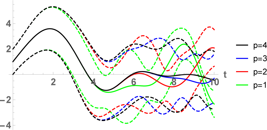
Expectation and confidence interval for the solution stochastic process, for orders of basis p = 1, 2, 3, 4. Example 4.1, assuming independent random data.
By using the random Fröbenius method from [16], an example of Airy’s differential equation with dependent random inputs is performed. It is set (A, Y0, Y1) to have a multivariate Gaussian distribution, with mean vector and covariance matrix given by
respectively. In Table 4, Table 5 and Table 6, the results obtained via adaptive gPC with p = 3, p = 4 (dependent case) and [16] are shown. Adaptive gPC converges for small order of basis p.
Approximation of 𝔼[X(t)]. Example 4.1, assuming dependent random data.
| t | gPC p = 3 | gPC p = 4 | Fröb. N = 4 | Fröb. N = 5 | dishonest | MC 50,000 | MC 100,000 |
|---|---|---|---|---|---|---|---|
| 0.00 | 1 | 1 | 1 | 1 | 1 | 1.00188 | 1.00597 |
| 0.25 | 1.49870 | 1.49870 | 1.49870 | 1.49870 | 1.49870 | 1.50166 | 1.50581 |
| 0.50 | 1.98755 | 1.98755 | 1.98755 | 1.98755 | 1.98752 | 1.99156 | 1.99575 |
| 0.75 | 2.45121 | 2.45121 | 2.45121 | 2.45121 | 2.45102 | 2.45622 | 2.46041 |
| 1.00 | 2.86895 | 2.86895 | 2.86895 | 2.86895 | 2.86818 | 2.87485 | 2.87900 |
| 1.25 | 3.21589 | 3.21589 | 3.21589 | 3.21589 | 3.21339 | 3.22247 | 3.22656 |
| 1.50 | 3.46503 | 3.46503 | 3.46503 | 3.46503 | 3.45812 | 3.47198 | 3.47601 |
| 1.75 | 3.59010 | 3.59010 | 3.59010 | 3.59010 | 3.57340 | 3.59700 | 3.60101 |
| 2.00 | 3.56914 | 3.56914 | 3.56915 | 3.56914 | 3.53286 | 3.57546 | 3.57949 |
Approximation of 𝕍[X(t)]. Example 4.1, assuming dependent random data.
| t | gPC p = 3 | gPC p = 4 | Fröb. N = 3 | Fröb. N = 4 | MC 50,000 | MC 100,000 |
|---|---|---|---|---|---|---|
| 0.00 | 1 | 1 | 1 | 1 | 0.999223 | 0.99992 |
| 0.25 | 1.30997 | 1.30997 | 1.30997 | 1.30997 | 1.30713 | 1.30991 |
| 0.50 | 1.72535 | 1.72535 | 1.72535 | 1.72535 | 1.71989 | 1.72525 |
| 0.75 | 2.21241 | 2.21241 | 2.21241 | 2.21241 | 2.20395 | 2.21230 |
| 1.00 | 2.72122 | 2.72122 | 2.72122 | 2.72122 | 2.70957 | 2.72125 |
| 1.25 | 3.19236 | 3.19236 | 3.19236 | 3.19236 | 3.17745 | 3.19283 |
| 1.50 | 3.57361 | 3.57361 | 3.57361 | 3.57361 | 3.55537 | 3.57484 |
| 1.75 | 3.84459 | 3.84459 | 3.84454 | 3.84458 | 3.82262 | 3.84669 |
| 2.00 | 4.04087 | 4.04087 | 4.04090 | 4.04086 | 4.01420 | 4.04342 |
Approximation of ℂov[X(t), X(s)] via adapted gPC with p = 3 and p = 4. Example 4.1, assuming dependent random data.
| t–s | 0 | 0.25 | 0.5 | 0.75 | 1 | 1.25 | 1.5 | 1.75 | 2 |
|---|---|---|---|---|---|---|---|---|---|
| 0 | 1. | 1.12389 | 1.24064 | 1.34181 | 1.41793 | 1.45914 | 1.45614 | 1.40144 | 1.29068 |
| 0.25 | 1.12389 | 1.30997 | 1.48771 | 1.64683 | 1.77533 | 1.86031 | 1.88919 | 1.85125 | 1.7394 |
| 0.5 | 1.24064 | 1.48771 | 1.72535 | 1.94152 | 2.12187 | 2.25061 | 2.31202 | 2.29226 | 2.18163 |
| 0.75 | 1.34181 | 1.64683 | 1.94152 | 2.21241 | 2.4431 | 2.61534 | 2.71062 | 2.71235 | 2.60832 |
| 1 | 1.41793 | 1.77533 | 2.12187 | 2.4431 | 2.72122 | 2.93619 | 3.06742 | 3.09609 | 3.00785 |
| 1.25 | 1.45914 | 1.86031 | 2.25061 | 2.61534 | 2.93619 | 3.19236 | 3.36219 | 3.42552 | 3.36639 |
| 1.5 | 1.45614 | 1.88919 | 2.31202 | 2.71062 | 3.06742 | 3.36219 | 3.57361 | 3.68135 | 3.66862 |
| 1.75 | 1.40144 | 1.85125 | 2.29226 | 2.71235 | 3.09609 | 3.42552 | 3.68135 | 3.84459 | 3.89856 |
| 2 | 1.29068 | 1.7394 | 2.18163 | 2.60832 | 3.00785 | 3.36639 | 3.66862 | 3.89856 | 4.04087 |
In Figure 2, we analyze the convergence of gPC expansions by depicting the expectation (solid line) and confidence interval (dashed lines) for X(t), where the confidence interval is constructed as mean ± deviation. Analogous comments to those from Figure 1 apply in this case again. For orders p = 3 and p = 4, the expectations agree up to time t = 6, while the standard deviations coincide until t = 4.6. For p = 2 and p = 3, the means are similar until t = 6, whereas the dispersion estimates start separating from t = 3.8. Finally, for p = 1 and p = 2, the approximations for the average statistic coincide till t = 4.5, and for the deviation statistic until t = 2.5.
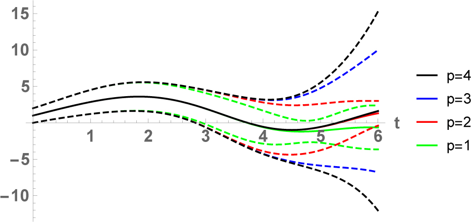
Expectation and confidence interval for the solution stochastic process, for orders of basis p = 1, 2, 3, 4. Example 4.1, assuming dependent random data.
Example 4.2
Consider the random differential equation
where γ1 ∼ Poisson(3), γ2 ∼ Uniform(0, 1), η1 ∼ Gamma(2, 2), Y0 = −1, Y1 ∼ Exponential(4), ξ1 ∼ Uniform(−8, 2) and g(t) = e−1/t1(0,∞)(t).
Proposition 2.1 ensures the existence and uniqueness of a sample path solution. To apply Proposition 2.2, one would need to truncate the supports of γ1 and η1. These truncations can be constructed on intervals as large as desired, in order to maintain the results.
The input random variables ζ1 = γ1, ζ2 = γ2, ζ3 = η1, ζ4 = ξ1 and ζ5 = Y1 are assumed to be independent. The involved functions are a1(t) = 1, a2(t) = t, b1(t) = 1, b2(t) = t, c0(t) = g(t) and c1(t) = cos(t). Notice that C(t) is not an analytic stochastic process, because g(t) is not a real analytic function. The random Fröbenius method is not applicable for the random IVP (15). However, we are going to see that adaptive gPC (independent case) with p = 6 and p = 7 provides reliable approximations of the expectation and covariance of X(t). We will compare the results with Monte Carlo simulation. In Table 7, Table 8 and Table 9 we show the estimates obtained.
Approximation of 𝔼[X(t)]. Example 4.2, assuming independent random data.
| t | gPC p = 6 | gPC p = 7 | dishonest | MC 50,000 | MC 100,000 |
|---|---|---|---|---|---|
| 0.00 | −1 | −1 | −1 | −1 | −1 |
| 0.25 | −0.930972 | −0.930972 | −0.931372 | −0.931035 | −0.930364 |
| 0.50 | −0.855779 | −0.855779 | −0.852372 | −0.855937 | −0.854386 |
| 0.75 | −0.780021 | −0.780021 | −0.759103 | −0.780573 | −0.778022 |
| 1.00 | −0.700758 | −0.700758 | −0.647653 | −0.702042 | −0.698437 |
| 1.25 | −0.609156 | −0.609156 | −0.518169 | −0.611266 | −0.606832 |
| 1.50 | −0.496445 | −0.496446 | −0.374486 | −0.499156 | −0.494407 |
| 1.75 | −0.359632 | −0.359635 | −0.222874 | −0.362532 | −0.358036 |
| 2.00 | −0.203726 | −0.203737 | −0.070806 | −0.206408 | −0.202560 |
Approximation of 𝕍[X(t)]. Example 4.2, assuming independent random data.
| t | gPC p = 6 | gPC p = 7 | MC 50,000 | MC 100,000 |
|---|---|---|---|---|
| 0.00 | 0 | 0 | 0 | 0 |
| 0.25 | 0.0114271 | 0.0114271 | 0.0115378 | 0.0114953 |
| 0.50 | 0.0897916 | 0.0897916 | 0.0904703 | 0.090160 |
| 0.75 | 0.236135 | 0.236136 | 0.237288 | 0.237066 |
| 1.00 | 0.371625 | 0.371639 | 0.372899 | 0.373058 |
| 1.25 | 0.426921 | 0.427021 | 0.428690 | 0.428342 |
| 1.50 | 0.388485 | 0.388899 | 0.391305 | 0.38978 |
| 1.75 | 0.289622 | 0.290720 | 0.293631 | 0.291429 |
| 2.00 | 0.182954 | 0.184922 | 0.187906 | 0.185917 |
Approximation of ℂov[X(t), X(s)] via adapted gPC with p = 7. Example 4.2, assuming independent random data.
| t–s | 0 | 0.25 | 0.5 | 0.75 | 1 | 1.25 | 1.5 | 1.75 | 2 |
|---|---|---|---|---|---|---|---|---|---|
| 0 | 0 | 0 | 0 | 0 | 0 | 0 | 0 | 0 | 0 |
| 0.25 | 0 | 0.0114271 | 0.0310997 | 0.0486065 | 0.0585142 | 0.0597207 | 0.0537473 | 0.042977 | 0.0295893 |
| 0.5 | 0 | 0.0310997 | 0.0897916 | 0.14431 | 0.176903 | 0.182770 | 0.165621 | 0.132554 | 0.0905903 |
| 0.75 | 0 | 0.0486065 | 0.14431 | 0.236136 | 0.293929 | 0.307634 | 0.281495 | 0.226547 | 0.154877 |
| 1 | 0 | 0.0585142 | 0.176903 | 0.293929 | 0.371639 | 0.394991 | 0.366485 | 0.29839 | 0.206021 |
| 1.25 | 0 | 0.0597207 | 0.182770 | 0.307634 | 0.394991 | 0.427021 | 0.403260 | 0.334311 | 0.235733 |
| 1.5 | 0 | 0.0537473 | 0.165621 | 0.281495 | 0.366485 | 0.403260 | 0.388899 | 0.330575 | 0.241178 |
| 1.75 | 0 | 0.042977 | 0.132554 | 0.226547 | 0.29839 | 0.334311 | 0.330575 | 0.29072 | 0.223109 |
| 2 | 0 | 0.0295893 | 0.0905903 | 0.154877 | 0.206021 | 0.235733 | 0.241178 | 0.223109 | 0.184922 |
In Figure 3, we focus on the convergence of gPC expansions. We depict the estimates of the expectations (solid line) and confidence intervals (dashed lines), with the rule mean ± deviation, for orders p = 4, 5, 6, 7. Note that convergence is achieved for t ∈ [0, 10].
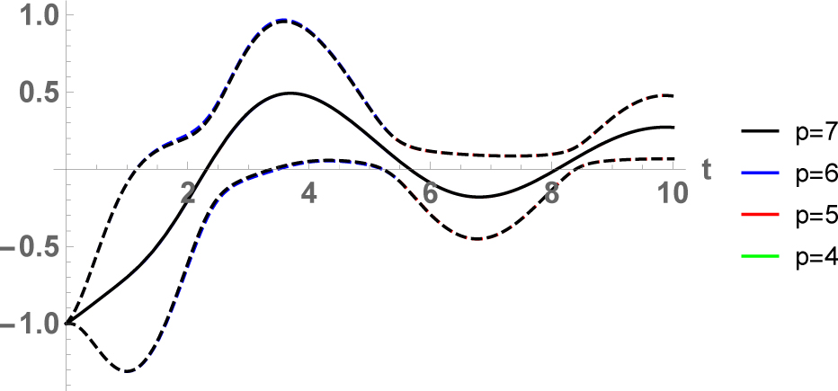
Expectation and confidence interval for the solution stochastic process, for orders of basis p = 4, 5, 6, 7. Example 4.2, assuming independent random data.
Example 4.3
Consider the random differential equation
where B(t) is a standard Brownian motion on [0, 1], C ∼ Poisson(2), and the initial conditions are distributed as Y0 ∼ Beta(1/2, 1/2) and Y1 = 0. These random inputs are assumed to be independent.
This stochastic system has a unique solution in the sample path sense, by Proposition 2.1. In principle, one cannot ensure the existence of a mean square solution, since the sample paths of Brownian motion are not bounded.
Consider the Karhunen-Loève expansion of Brownian motion [25, p. 216]:
where ξ1, ξ2, … are independent and Normal(0, 1) random variables. The series is understood in L2([0, 1] × Ω). We truncate the Karhunen-Loève expansion so that B(t) will have the form in (2). If we take dB = 7, we are capturing more than 97% of the total variance of X. Thus, we take
The random inputs become ζ1 = ξ1, …, ζ7 = ξ7, ζ8 = C and ζ9 = Y0, with functions
Notice that, if one truncates ξ1, …, ξ7 to a large but bounded support, Proposition 2.2 entails that there exists a solution stochastic process in the mean square sense.
In Table 10, Table 11 and Table 12, we show the results obtained by adaptive gPC with p = 2, p = 3 and Monte Carlo simulation. Similar estimates are obtained for p = 2 and p = 3, which agrees with the convergence of gPC-based representations.
Approximation of 𝔼[X(t)]. Example 4.3, assuming independent random data.
| t | gPC p = 2 | gPC p = 3 | dishonest | MC 50,000 | MC 100,000 |
|---|---|---|---|---|---|
| 0.00 | 0.5 | 0.5 | 0.5 | 0.499302 | 0.499056 |
| 0.25 | 0.562504 | 0.562504 | 0.5625 | 0.561732 | 0.561438 |
| 0.50 | 0.75014 | 0.75014 | 0.75 | 0.749196 | 0.748740 |
| 0.75 | 1.06365 | 1.06365 | 1.0625 | 1.06245 | 1.06179 |
| 1.00 | 1.50536 | 1.50536 | 1.5 | 1.50396 | 1.50311 |
Approximation of 𝕍[X(t)]. Example 4.3, assuming independent random data.
| t | gPC p = 2 | gPC p = 3 | MC 50,000 | MC 100,000 |
|---|---|---|---|---|
| 0.00 | 0.125 | 0.125 | 0.124849 | 0.124826 |
| 0.25 | 0.126974 | 0.126974 | 0.126883 | 0.126841 |
| 0.50 | 0.157008 | 0.157008 | 0.157267 | 0.157033 |
| 0.75 | 0.290263 | 0.290265 | 0.291811 | 0.290766 |
| 1.00 | 0.664551 | 0.664592 | 0.670067 | 0.666466 |
Approximation of ℂov[X(t), X(s)] via adapted gPC with p = 3. Example 4.3, assuming independent random data.
| t–s | 0 | 0.25 | 0.5 | 0.75 | 1 |
|---|---|---|---|---|---|
| 0 | 0.125 | 0.125001 | 0.125033 | 0.125248 | 0.126043 |
| 0.25 | 0.125001 | 0.126974 | 0.132949 | 0.143104 | 0.157885 |
| 0.5 | 0.125033 | 0.132949 | 0.157008 | 0.197634 | 0.255578 |
| 0.75 | 0.125248 | 0.143104 | 0.197634 | 0.290265 | 0.422829 |
| 1 | 0.126043 | 0.157885 | 0.255578 | 0.422829 | 0.664592 |
In Figure 4, we show graphically the convergence of gPC expansions on [0, 1]: we plot the approximate expectations (solid line) and confidence intervals (dashed lines) for X(t), where the confidence interval is constructed as mean ± deviation. For p = 1, 2, 3, no differences in the estimates are observed.
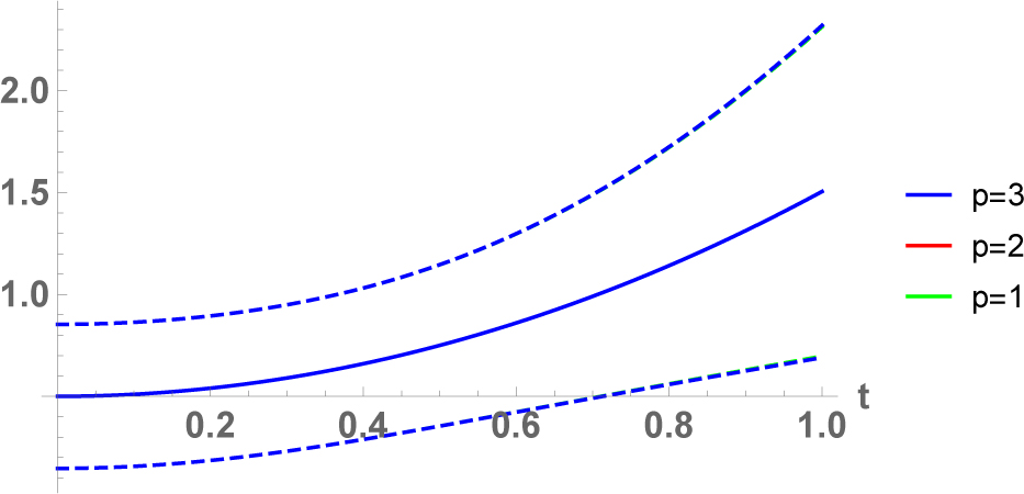
Expectation and confidence interval for the solution stochastic process, for orders of basis p = 1, 2, 3. Example 4.3, assuming independent random data.
5 Conclusions
In this paper, we have quantified computationally the uncertainty of random non-autonomous second-order linear differential equations via adaptive gPC. After reviewing adaptive gPC from the extant literature, we have provided a methodology and an algorithm to approximate computationally the expectation and covariance of the solution stochastic process. The hypotheses from our algorithm allow both independent and dependent random parameter inputs, being both absolutely continuous or discrete with infinitely many point masses. The generality of our computational results allows the random input coefficients to be truncated random power series or truncated Karhunen-Loève expansions. The former case permits comparing our methodology with the random Fröbenius method, an approach already used in the literature with particular random second-order linear differential equations, and Monte Carlo simulation. A wide variety of examples show that adaptive gPC becomes successful quantifying the uncertainty of random non-autonomous second-order linear differential equations, even when the random Fröbenius method is not applicable.
Acknowledgement
This work has been supported by the Spanish Ministerio de Economía y Competitividad grant MTM2017–89664–P. Marc Jornet acknowledges the doctorate scholarship granted by Programa de Ayudas de Investigación y Desarrollo (PAID), Universitat Politècnica de València. The authors are grateful for the valuable comments raised by the reviewer, which have improved the final version of the paper.
Conflict of interest
Conflict of Interest Statement: The authors declare that there is no conflict of interests regarding the publication of this article.
References
[1] Strand J.L., Random Ordinary Differential Equations, J. Differ. Equ., 1970, 7, 538–553.10.1016/0022-0396(70)90100-2Search in Google Scholar
[2] Soong T.T., Random Differential Equations in Science and Engineering, 1973, New York: Academic Press.Search in Google Scholar
[3] Xiu D., Numerical Methods for Stochastic Computations. A Spectral Method Approach, 2010, Princeton University Press.10.1515/9781400835348Search in Google Scholar
[4] Xiu D., Karniadakis G.E, The Wiener-Askey polynomial chaos for stochastic differential equations, SIAM J. Sci. Comput., 2002, 24 (2), 619–644.10.1137/S1064827501387826Search in Google Scholar
[5] Williams M.M.R., Polynomial chaos functions and stochastic differential equations, Ann. Nucl. Energy, 2006, 33 (9), 774–785.10.1016/j.anucene.2006.04.005Search in Google Scholar
[6] Chen-Charpentier B.M., Stanescu D., Epidemic models with random coefficients, Math. Comput. Model., 2010, 52 (7–8), 1004–1010.10.1016/j.mcm.2010.01.014Search in Google Scholar
[7] Chen-Charpentier B.M., Cortés J.C., Licea J.A., Romero J.V., Roselló M.D., Santonja F.J., Villanueva R.J., Constructing adaptive generalized polynomial chaos method to measure the uncertainty in continuous models: A computational approach, Math. Comput. Simulat., 2015, 109, 113–129.10.1016/j.matcom.2014.09.002Search in Google Scholar
[8] Cortés J.C., Romero J.V., Roselló M.D., Villanueva R.J., Improving adaptive generalized polynomial chaos method to solve nonlinear random differential equations by the random variable transformation technique, Commun. Nonlinear Sci. Numer. Simulat., 2017, 50, 1–15.10.1016/j.cnsns.2017.02.011Search in Google Scholar
[9] Cortés J.C., Romero J.V., Roselló M.D., Santonja F.J., Villanueva R.J., Solving Continuous Models with Dependent Uncertainty: A Computational Approach, Abstr. Appl. Anal., 2013.10.1155/2013/983839Search in Google Scholar
[10] Cortés J.C., Navarro-Quiles A., Romero J.V., Roselló M.D., Probabilistic solution of random autonomous first-order linear systems of ordinary differential equations, Rom. Rep. Phys., 2016, 68 (4), 1397–1406.10.1016/j.aml.2016.12.015Search in Google Scholar
[11] Gottlieb D., Xiu D., Galerkin method for wave equations with uncertain coefficients, Commun. Comput. Phys., 2008, 3 (2), 505–518.Search in Google Scholar
[12] Ernst O.G., Mugler A., Starkloff H.J., Ullmann E., On the convergence of generalized polynomial chaos expansions, ESAIM-Math. Model. Num., 2012, 46 (2), 317–339.10.1051/m2an/2011045Search in Google Scholar
[13] Shi W., Zhang C., Error analysis of generalized polynomial chaos for nonlinear random ordinary differential equations, Appl. Numer. Math., 2012, 62 (12), 1954–1964.10.1016/j.apnum.2012.08.007Search in Google Scholar
[14] Shi W., Zhang C., Generalized polynomial chaos for nonlinear random delay differential equations, Appl. Numer. Math., 2017, 115, 16–31.10.1016/j.apnum.2016.12.004Search in Google Scholar
[15] Calatayud J., Cortés J.C., Jornet M., On the convergence of adaptive gPC for non-linear random difference equations: Theoretical analysis and some practical recommendations, J. Nonlinear Sci. App., 2018, 11 (9), 1077–1084.10.22436/jnsa.011.09.06Search in Google Scholar
[16] Cortés J.C., Jódar L., Camacho F., Villafuerte L., Random Airy type differential equations: Mean square exact and numerical solutions, Comput. Math. Appl., 2010, 60, 1237–1244.10.1016/j.camwa.2010.05.046Search in Google Scholar
[17] Calbo G., Cortés J.C., Jódar L., Random Hermite differential equations: Mean square power series solutions and statistical properties, Appl. Math. Comput., 2011, 218 (7), 3654–3666.10.1016/j.amc.2011.09.008Search in Google Scholar
[18] Calbo G., Cortés J.C., Jódar L., Villafuerte L., Solving the random Legendre differential equation: Mean square power series solution and its statistical functions, Comput. Math. Appl., 2011, 61 (9), 2782–2792.10.1016/j.camwa.2011.03.045Search in Google Scholar
[19] Calatayud J., Cortés J.C., Jornet M., Improving the approximation of the first and second order statistics of the response process to the random Legendre differential equation, 2018, arXiv preprint, arXiv:1807.03141.10.1007/s00009-019-1338-6Search in Google Scholar
[20] Cortés J.C., Jódar L., Company R., Villafuerte L., Laguerre random polynomials: definition, differential and statistical properties, Utilitas Mathematica, 2015, 98, 283–295.Search in Google Scholar
[21] Cortés J.C., Jódar L., Villafuerte L., Mean square solution of Bessel differential equation with uncertainties, J. Comput. Appl. Math., 2017, 309 (1), 383–395.10.1016/j.cam.2016.01.034Search in Google Scholar
[22] Calatayud J., Cortés J.C., Jornet M., Villafuerte L., Random non-autonomous second order linear differential equations: mean square analytic solutions and their statistical properties, Adv. Differ. Equ., 2018, 392, 1–29.10.1186/s13662-018-1848-8Search in Google Scholar
[23] Calatayud J., Cortés J.C., Jornet M., Some notes to extend the study on random non-autonomous second order linear differential equations appearing in Mathematical Modeling, Math. Comput. Appl., 2018, 23 (4), 76–89.10.3390/mca23040076Search in Google Scholar
[24] Golmankhaneh A.K., Porghoveh N.A., Baleanu D., Mean square solutions of second-order random differential equations by using homotopy analysis method, Rom. Rep. Phys., 2013, 65 (2).Search in Google Scholar
[25] Lord G.J., Powell C.E., Shardlow T., An Introduction to Computational Stochastic PDEs, 2014, New York: Cambridge Texts in Applied Mathematics, Cambridge University Press.10.1017/CBO9781139017329Search in Google Scholar
[26] Hale J.K., Ordinary Differential Equations (2nd ed.), 1980, Malabar: Robert E. Krieger Publishing Company.Search in Google Scholar
[27] Henderson D., Plaschko P., Stochastic Differential Equations in Science and Engineering, 2006, Singapore: World Scientific.10.1142/5806Search in Google Scholar
[28] Vallée O., Soares M., Airy Functions and Applications to Physics, 2004, London: Imperial College Press.10.1142/p345Search in Google Scholar
© 2018 Calatayud et al., published by De Gruyter
This work is licensed under the Creative Commons Attribution-NonCommercial-NoDerivatives 4.0 License.
Articles in the same Issue
- Regular Articles
- Algebraic proofs for shallow water bi–Hamiltonian systems for three cocycle of the semi-direct product of Kac–Moody and Virasoro Lie algebras
- On a viscous two-fluid channel flow including evaporation
- Generation of pseudo-random numbers with the use of inverse chaotic transformation
- Singular Cauchy problem for the general Euler-Poisson-Darboux equation
- Ternary and n-ary f-distributive structures
- On the fine Simpson moduli spaces of 1-dimensional sheaves supported on plane quartics
- Evaluation of integrals with hypergeometric and logarithmic functions
- Bounded solutions of self-adjoint second order linear difference equations with periodic coeffients
- Oscillation of first order linear differential equations with several non-monotone delays
- Existence and regularity of mild solutions in some interpolation spaces for functional partial differential equations with nonlocal initial conditions
- The log-concavity of the q-derangement numbers of type B
- Generalized state maps and states on pseudo equality algebras
- Monotone subsequence via ultrapower
- Note on group irregularity strength of disconnected graphs
- On the security of the Courtois-Finiasz-Sendrier signature
- A further study on ordered regular equivalence relations in ordered semihypergroups
- On the structure vector field of a real hypersurface in complex quadric
- Rank relations between a {0, 1}-matrix and its complement
- Lie n superderivations and generalized Lie n superderivations of superalgebras
- Time parallelization scheme with an adaptive time step size for solving stiff initial value problems
- Stability problems and numerical integration on the Lie group SO(3) × R3 × R3
- On some fixed point results for (s, p, α)-contractive mappings in b-metric-like spaces and applications to integral equations
- On algebraic characterization of SSC of the Jahangir’s graph 𝓙n,m
- A greedy algorithm for interval greedoids
- On nonlinear evolution equation of second order in Banach spaces
- A primal-dual approach of weak vector equilibrium problems
- On new strong versions of Browder type theorems
- A Geršgorin-type eigenvalue localization set with n parameters for stochastic matrices
- Restriction conditions on PL(7, 2) codes (3 ≤ |𝓖i| ≤ 7)
- Singular integrals with variable kernel and fractional differentiation in homogeneous Morrey-Herz-type Hardy spaces with variable exponents
- Introduction to disoriented knot theory
- Restricted triangulation on circulant graphs
- Boundedness control sets for linear systems on Lie groups
- Chen’s inequalities for submanifolds in (κ, μ)-contact space form with a semi-symmetric metric connection
- Disjointed sum of products by a novel technique of orthogonalizing ORing
- A parametric linearizing approach for quadratically inequality constrained quadratic programs
- Generalizations of Steffensen’s inequality via the extension of Montgomery identity
- Vector fields satisfying the barycenter property
- On the freeness of hypersurface arrangements consisting of hyperplanes and spheres
- Biderivations of the higher rank Witt algebra without anti-symmetric condition
- Some remarks on spectra of nuclear operators
- Recursive interpolating sequences
- Involutory biquandles and singular knots and links
- Constacyclic codes over 𝔽pm[u1, u2,⋯,uk]/〈 ui2 = ui, uiuj = ujui〉
- Topological entropy for positively weak measure expansive shadowable maps
- Oscillation and non-oscillation of half-linear differential equations with coeffcients determined by functions having mean values
- On 𝓠-regular semigroups
- One kind power mean of the hybrid Gauss sums
- A reduced space branch and bound algorithm for a class of sum of ratios problems
- Some recurrence formulas for the Hermite polynomials and their squares
- A relaxed block splitting preconditioner for complex symmetric indefinite linear systems
- On f - prime radical in ordered semigroups
- Positive solutions of semipositone singular fractional differential systems with a parameter and integral boundary conditions
- Disjoint hypercyclicity equals disjoint supercyclicity for families of Taylor-type operators
- A stochastic differential game of low carbon technology sharing in collaborative innovation system of superior enterprises and inferior enterprises under uncertain environment
- Dynamic behavior analysis of a prey-predator model with ratio-dependent Monod-Haldane functional response
- The points and diameters of quantales
- Directed colimits of some flatness properties and purity of epimorphisms in S-posets
- Super (a, d)-H-antimagic labeling of subdivided graphs
- On the power sum problem of Lucas polynomials and its divisible property
- Existence of solutions for a shear thickening fluid-particle system with non-Newtonian potential
- On generalized P-reducible Finsler manifolds
- On Banach and Kuratowski Theorem, K-Lusin sets and strong sequences
- On the boundedness of square function generated by the Bessel differential operator in weighted Lebesque Lp,α spaces
- On the different kinds of separability of the space of Borel functions
- Curves in the Lorentz-Minkowski plane: elasticae, catenaries and grim-reapers
- Functional analysis method for the M/G/1 queueing model with single working vacation
- Existence of asymptotically periodic solutions for semilinear evolution equations with nonlocal initial conditions
- The existence of solutions to certain type of nonlinear difference-differential equations
- Domination in 4-regular Knödel graphs
- Stepanov-like pseudo almost periodic functions on time scales and applications to dynamic equations with delay
- Algebras of right ample semigroups
- Random attractors for stochastic retarded reaction-diffusion equations with multiplicative white noise on unbounded domains
- Nontrivial periodic solutions to delay difference equations via Morse theory
- A note on the three-way generalization of the Jordan canonical form
- On some varieties of ai-semirings satisfying xp+1 ≈ x
- Abstract-valued Orlicz spaces of range-varying type
- On the recursive properties of one kind hybrid power mean involving two-term exponential sums and Gauss sums
- Arithmetic of generalized Dedekind sums and their modularity
- Multipreconditioned GMRES for simulating stochastic automata networks
- Regularization and error estimates for an inverse heat problem under the conformable derivative
- Transitivity of the εm-relation on (m-idempotent) hyperrings
- Learning Bayesian networks based on bi-velocity discrete particle swarm optimization with mutation operator
- Simultaneous prediction in the generalized linear model
- Two asymptotic expansions for gamma function developed by Windschitl’s formula
- State maps on semihoops
- 𝓜𝓝-convergence and lim-inf𝓜-convergence in partially ordered sets
- Stability and convergence of a local discontinuous Galerkin finite element method for the general Lax equation
- New topology in residuated lattices
- Optimality and duality in set-valued optimization utilizing limit sets
- An improved Schwarz Lemma at the boundary
- Initial layer problem of the Boussinesq system for Rayleigh-Bénard convection with infinite Prandtl number limit
- Toeplitz matrices whose elements are coefficients of Bazilevič functions
- Epi-mild normality
- Nonlinear elastic beam problems with the parameter near resonance
- Orlicz difference bodies
- The Picard group of Brauer-Severi varieties
- Galoisian and qualitative approaches to linear Polyanin-Zaitsev vector fields
- Weak group inverse
- Infinite growth of solutions of second order complex differential equation
- Semi-Hurewicz-Type properties in ditopological texture spaces
- Chaos and bifurcation in the controlled chaotic system
- Translatability and translatable semigroups
- Sharp bounds for partition dimension of generalized Möbius ladders
- Uniqueness theorems for L-functions in the extended Selberg class
- An effective algorithm for globally solving quadratic programs using parametric linearization technique
- Bounds of Strong EMT Strength for certain Subdivision of Star and Bistar
- On categorical aspects of S -quantales
- On the algebraicity of coefficients of half-integral weight mock modular forms
- Dunkl analogue of Szász-mirakjan operators of blending type
- Majorization, “useful” Csiszár divergence and “useful” Zipf-Mandelbrot law
- Global stability of a distributed delayed viral model with general incidence rate
- Analyzing a generalized pest-natural enemy model with nonlinear impulsive control
- Boundary value problems of a discrete generalized beam equation via variational methods
- Common fixed point theorem of six self-mappings in Menger spaces using (CLRST) property
- Periodic and subharmonic solutions for a 2nth-order p-Laplacian difference equation containing both advances and retardations
- Spectrum of free-form Sudoku graphs
- Regularity of fuzzy convergence spaces
- The well-posedness of solution to a compressible non-Newtonian fluid with self-gravitational potential
- On further refinements for Young inequalities
- Pretty good state transfer on 1-sum of star graphs
- On a conjecture about generalized Q-recurrence
- Univariate approximating schemes and their non-tensor product generalization
- Multi-term fractional differential equations with nonlocal boundary conditions
- Homoclinic and heteroclinic solutions to a hepatitis C evolution model
- Regularity of one-sided multilinear fractional maximal functions
- Galois connections between sets of paths and closure operators in simple graphs
- KGSA: A Gravitational Search Algorithm for Multimodal Optimization based on K-Means Niching Technique and a Novel Elitism Strategy
- θ-type Calderón-Zygmund Operators and Commutators in Variable Exponents Herz space
- An integral that counts the zeros of a function
- On rough sets induced by fuzzy relations approach in semigroups
- Computational uncertainty quantification for random non-autonomous second order linear differential equations via adapted gPC: a comparative case study with random Fröbenius method and Monte Carlo simulation
- The fourth order strongly noncanonical operators
- Topical Issue on Cyber-security Mathematics
- Review of Cryptographic Schemes applied to Remote Electronic Voting systems: remaining challenges and the upcoming post-quantum paradigm
- Linearity in decimation-based generators: an improved cryptanalysis on the shrinking generator
- On dynamic network security: A random decentering algorithm on graphs