
Time parallelization scheme with an adaptive time step size for solving stiff initial value problems
-
Sunyoung Bu


Abstract
In this paper, we introduce a practical strategy to select an adaptive time step size suitable for the parareal algorithm designed to parallelize a numerical scheme for solving stiff initial value problems. For the adaptive time step size, a technique to detect stiffness of a given system is first considered since the step size will be chosen according to the extent of stiffness. Finally, the stiffness detection technique is applied to an initial prediction step of the parareal algorithm, and select an adaptive step size to each time interval according to the stiffness. Several numerical experiments demonstrate the efficiency of the proposed method.
1 Introduction
We consider numerical techniques to solve stiff initial value problems (IVPs) given by
where f has continuously bounded partial derivatives up to required order for the developed numerical method. The stiff systems are broadly classified into two categories - one is to have stiff components in just a given system and the other is to have the components in both the system and its solution. In the first case, solutions of the system behaves smoothly as time is increasing so it can be easily solved by any implicit scheme with an appropriate step size. On the other hand, the solutions of the given system in the second case have stiff components expressed as irregularities or sharp fronts in some or whole time intervals. In the intervals, we carefully handle a numerical scheme since the solutions are very rapidly changed. Most interesting research topics, induced from the real applications such as fluid dynamics, molecular dynamics, plasma or other physics, are related with the second case.
There are lots of numerical strategies to find efficient and accurate solutions of the stiff systems. In this paper, we focus on the parallelization scheme to find the efficient solutions of the stiff IVPs. Time parallelization scheme has received a lot of attention over the past few years and several parallelization schemes have been proposed [1, 2, 3]. Especially in 2001, a new algorithm which was named parareal algorithm for the solution of time dependent differential equations in parallel was introduced [4]. It can be defined by
where the subscript n refers to the time subdomain number, the superscript k refers to the iteration number. F represents a fine propagator, that is, a more accurate solution on a fine grid in time interval [tn, tn+1] with an initial value
In the parareal algorithm, there is an important assumption that there are an infinite number of processors to use, so each processor is assigned to each different time interval with a uniform time step size. However, only a few finite number of processors can be provided in practice. Even if an infinite number of processors are provided, it is not efficient to assign the uniform step size on each processor without any consideration on the property of the problem, especially for stiff systems or partial differential equations (PDEs) having sharp front. That is, it is more efficient that a larger time step size is assigned for smooth or non-stiff regions in solutions, while a smaller time step size is needed for shock or stiff regions. Therefore, the usage of adaptive step sizes is very important issue to improve the efficiency of the parareal algorithm. Related to this issue, many researchers have attempted to find a suitable way to automatically detect stiffness [7].
The aims of this paper are to introduce a criterion to detect stiffness and to develop a scheme for finding an adaptive time step size according to the extent of stiffness in each interval. First of all, for the given system, we need to split the stiff and non-stiff parts in a given time domain. There are various ways to detect stiffness. For simplicity’s sake, we examine a gradient ratio of a given system to split the stiff and non-stiff parts. Once the stiff regions is detected, the corresponding step size should be automatically controlled. So, the time intervals in stiff regions should be gradually shrank depending on the extent of the stiffness, while those in non-stiff regions are comparatively stretched. Based on these processes, an appropriate time step size for the parareal algorithm is chosen in the sequential step depending on the stiffness at each time interval. Note that in the traditional parareal algorithm, a G-propagator approximates initial values for all time intervals sequentially, with having a uniform step size at the initialization step.
Additionally, a theoretical analysis of the parareal algorithm shows that the stability of the method depends on the choice of G-propagator [5, 8]. Especially, for solving highly stiff problem, G-propagator should be satisfied an L-stability. Also, each time interval is determined in the initialization step with a G-propagator, the computational cost for G-propagator should be small enough. Overall, Backward Euler (BE) method will be a good candidate for the G-propagator, since BE is unconditionally stable, its computational costs is relatively small and it has L-stability [9], where it can unconditionally fulfill the stability condition of the parareal methods with less computational costs.
This paper is organized as follows. In Sec. 2, we briefly describe the original parareal technique and the improved parareal algorithms based on the original one. In Sec. 3, we introduce several parameters for detecting degree of stiffness in each interval and discuss a strategy to select adaptive time step size using stiffness detection to improve the overall efficiency of the parareal algorithm. In Sec. 4, preliminary numerical results are presented to show the efficiency of the proposed scheme. Finally in Sec. 5, future research directions are provided.
2 Parareal method
In this section, we briefly review the original parareal algorithm and the improved parareal algorithms based on the traditional algorithm.
2.1 Parareal algorithm
As in general parareal algorithm, we assume the time interval [0, T] is divided into Np intervals with each interval being assigned to a different processor denoted processors P1 through PNp. On each interval, the parareal method iteratively computes a succession of approximation
The parareal method begins by sequentially computing
Once each processor has a value
The method proceeds iteratively alternating between the parallel computation of F(tn+1,tn,
2.2 Improved parareal methods
In this subsection, we briefly introduce improved versions of parareal methods to develop for overcoming limitations of the original parareal algorithm.
Although the original parareal algorithm enables us to parallelize numerical algorithms for solving initial value problems, its efficiency is controversial since the low parallel efficiency which is bounded by 1/K, where K is the parareal iterations needed to converge to the desired accuracy. Note that K must be at least 2, the efficiency of the original parareal scheme is less than 50 percents and even worse in practice. To improve the low parallel efficiency for the parareal algorithm, several improved algorithms are developed [2, 5, 11], in which various deferred correction (DC) techniques are embedded into the parareal framework. In [2, 11], a hybrid parareal spectral deferred correction method was introduced in which spectral deferred correction (SDC) strategies are utilized within the parareal iteration, as a F-propagator. Also, in [5], two different deferred correction schemes, modified DC technique combined with Backward Euler (BE) method and Krylov deferred correction (KDC) [10], are used for G and F propagators in the parareal framework, similar to the hybrid parareal spectral deferred correction method. Commonly in [2, 5, 11], instead of directly using the SDC scheme or KDC scheme requiring several iterations (SDC sweeps in SDC or Newton-Krylov iterations in KDC) in serial, the F-propagator in each parareal iteration performs one or a few SDC sweeps or Newton-Krylov iterations on the solution from the previous parareal iteration. As the parareal iterations converge, the F solution still converges to the high-accuracy SDC or KDC solution.
The advantage of these schemes is that the F-propagator becomes much cheaper by combining the parareal iterations and DC iterations, compared to a full accurate solver. Because the DC iterations (SDC sweeps in SDC or Newton-Krylov iterations in KDC) are overlapped with the parareal iteration, so the hybrid parareal schemes can unite the two different iterations (DC and parareal iterations) [2, p. 281]. Typically, the original efficiency is bounded by 1/K, where K is the number of iterations for the parallel iterations to converge. However, the parallel efficiency of the hybrid parareal SDC or KDC is about Ks/K, where Ks is the number of iterations required of the serial SDC or KDC method to converge to a given tolerance. Note that the hybrid parareal SDC method is a reasonably good choice for non-stiff systems and parareal KDC method is suitable for stiff systems since KDC was developed to overcome the limitation of SDC for stiffness.
3 Algorithm
In the parareal algorithm, all processors are typically initialized by using the coarse propagator in a serial way to yield a low accuracy initial condition on each interval which is assigned to each processor. So, all processors except the first one are idle until passed an initial condition from the previous processor and the idle time is inevasible.
3.1 Stiffness detection
We now describe a parameter which dictates whether there exists a stiffness of a given system in a given time interval. Since stiffness implies that the given system has two different time scales. That is, a rate of maximum and minimum value of derivatives for the system in some interval is quite big, then we prescribe that it is stiff in the interval. In this respect, this can be easily done by introducing the following measure related to the gradient for the given problem :
where n is the dimension of the given system.
Note that we restrict the stiffness to the case when stiffness is on the problem and solution. That is, we need to check the change rate of κ(t) since it says whether any big change exists between the previous interval and the current one. This allows us to approximate a conditioning parameter γ(h) in each interval as follows:
where h = tm+1 − tm. We can easily check that γ(h) goes to 0 when there is a big difference between κ(tm) and κ(tm+1) due to big change in the interval [tm, tm+1]. Also, κ(tm) and κ(tm+1) have quite similar values, γ(h) goes to 1. That is, the parameter γ(h) can be used to detect the stiffness in the interval [tm, tm+1], so we say it “stiffness ratio”. Therefore, the stiffness ratio γ(h) is used to determine a time step size h according to the degree of the stiffness, since the ratio γ(h) is relatively small when solutions in a given time interval are rapidly changed and γ(h) is large when a change rate of solutions is increasingly small. Note that “the change rate of solutions is small” means that the solutions are smooth in that interval, so the time step size is allowed to be large. Hence the time step size can be selected adaptively small and increasingly large when the stiffness ratio γ(h) is small and relatively large, respectively.
3.2 Adaptive step size selection
For a code implementation, stiffness criteria to choose time step sizes are needed to be set up. When the ratio γ(h) is close to 1, the step size is expanded and when the ratio goes to 0, the step size should be shortened. For the sake of simplicity, we amplify the step size twice when the stiffness ration is 1, which means that there is no difference of κ(t) in an interval. In addition, the step size is reduced by half when the stiffness ratio is halved. Using these conditions, we simply set up the following criterion to choose a new time step size hnew as follows:
where hmax and hmin are constant factors to avoid too fast increase and decrease of the time step, respectively.
Based on the parameters and the discussion above, we get the following algorithm to select new step size as follows:
Algorithm for step size selection
Remark: The algorithm is designed to adaptively choose time step size for G-propagator in the parereal scheme. [t0, tfinal] is the required integration interval, and y0 is a given initial value.
Initialize h0, told:= t0.
Set tnew:= told + h. If tnew > tfinal, then exit.
Perform the Backward Euler method with having h and yold and approximate ynew.
hnew = min(hmax, max(hmin, 2h ⋅ γ(h)2))
Setting h = hnew, told := tnew and yold := ynew, go to step 3.
3.3 Parareal algorithm with the proposed adaptive step size controller
Based on the new step size controller with the stiffness detection discussed in the previous subsections, we present the enhanced parareal methods with adaptive step size. First of all, we assume the time interval of interest [0, T] is divided into N uniform intervals, and each interval [ti, ti+1] is assigned to a corresponding processor Pi. Note that
Predictor Step Decide initial values and step sizes in a serial way
Starting with the initial value y0 and h0,
Get the initial value
Using G-propagator, calculate the initial approximation
Using the step size selection technique discussed above, calculate a new step size hnew based on κ and γ.
Send the
Corrector Step Parallel Iteration (k + 1 step) for k = 0, …, N − 1
Using a higher order method, compute F(tn+1, tn,
After the approximation value
Using G-propagator with a new initial value
Update
where G(tn+1, tn,
4 Numerical results
In this section, preliminary numerical results are presented to examine the convergence behavior and efficiency of the enhanced parareal scheme, compared to the standard implementation of the original parareal scheme.
4.1 Robertson example
As the first example, we solve a classical problem due to Robertson which describes the kinetics of an autocatalytic reaction given by Robertson. Its system consists of a stiff system of 3 nonlinear ODEs given by
The initial vector y0 is given by [1, 0, 0]T. In this experiment, we march from t = 0 to tf = 1 with initial step size h0 = 1e − 4. To investigate the effectiveness of the proposed scheme, we simply experiment with the adaptive mesh selection using Backward Euler (BE) method and compare the accuracy of the proposed scheme that of the existing method (built-in Matlab function -ode15s).
Note that in this experiment, BE is used as a test method since BE is employed for G-propagator of the parareal algorithm in this paper. Fig. 1(a) shows that the proposed step size controller can solve the problem and its result is quite close to that from the existing method ode15s.
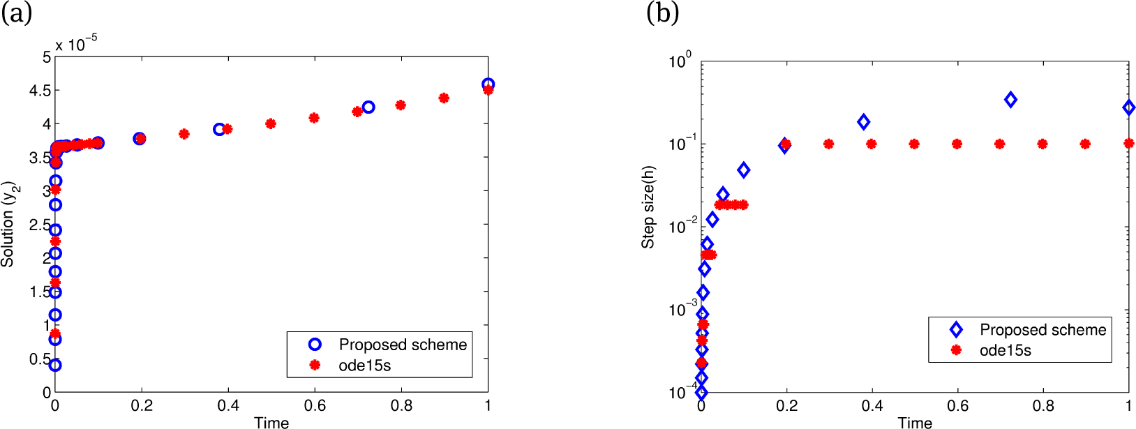
Comparison of (a) solution and (b) corresponding time step size for proposed scheme and existing method (ode15s)
Note that we just plot the second component of the solution set since the stiffness is on the second component. Also the stiffness is near t = 0, so we expect the step size is chosen relatively small in this region. For this, we plot the time step size by the proposed scheme over the time domain and compare it with that obtained by the existing method.
Fig. 1(b) shows that only 21 time steps are needed to reach the final time with the proposed scheme, while 104 time steps are required with uniform grid used in the original parareal scheme and 30 time steps with the existing scheme using adaptive time step size. Also, as seen in the figure, larger time step sizes are allowed by the proposed technique in non-stiff parts as desired.
Now we apply the adaptive mesh selection strategy to the parareal algorithm with KDC as a F-propagator and BE as a G-propagator. Also, for the experiment, the KDC methods with 4 Radau II nodes are employed, and each parareal iteration performs the 2 outer Newton iterations for desired efficiency and the other conditions such as the tolerance for the Newton-Krylov methods or nonlinear solvers are fixed for all simulations. We use a reference solution obtained from KDC scheme with 8 Radau II node and full outer Newton iterations.
To examine the convergence behavior of stiff parts, only 10 processors are used and corresponding final time point is 0.00125. In Fig. 2, we plot the error at the final time (t = 0.00125) versus the parareal iterations with an initial step size 104. It can be seen that after a certain number of parareal iterations, the error levels reach a certain tolerance level even for stiff parts. It also shows that to reach the final time 0.00125 using uniform grid with a step size h = 104, it requires 10 processors which is the same number of processors needed for the adaptive mesh parareal scheme. Hence, it must be noted that even using adaptive step sizes, the step sizes in stiff parts should become small enough.
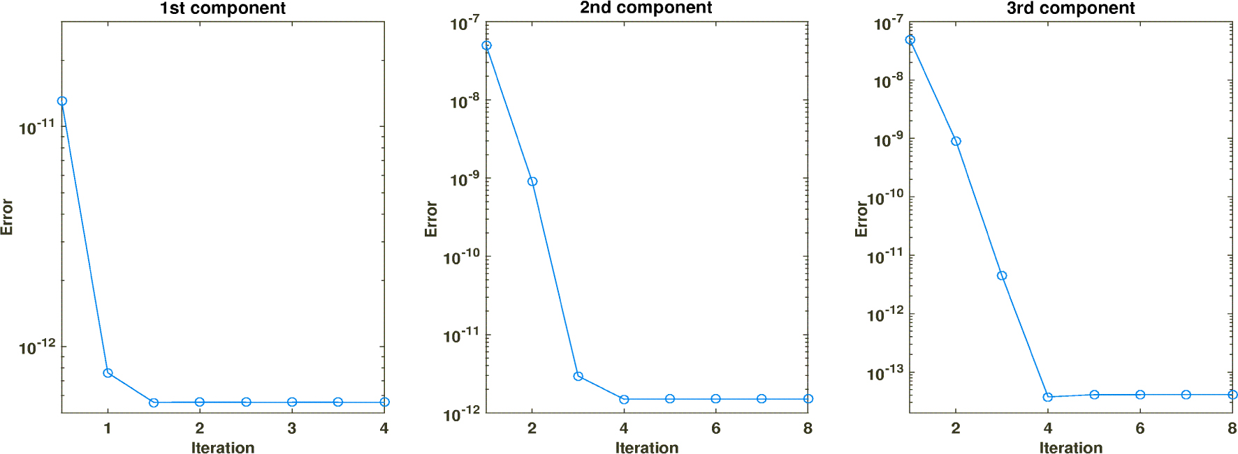
Convergence behavior of parareal iterations for each component of the given system
4.2 Van der Pol problem
This problem, that models the behavior in an electronic circuit, can be described as a system of two equations given by
where y(t) = [y1(t), y2(t)]T ∈ ℝ2 and f is defined by
with initial condition y0 = [2, 0]T. From the second component of f, it can be seen that the smaller ϵ is, the stronger stiffness of problem is. For the test, we take ϵ = 1/1000 and initial time step size h0 = 10−4.
To examine the effectiveness of the proposed scheme, we plot the solution y1 over the time domain and its corresponding step size h in Fig. 5. The figure shows that the step size is adaptively chosen to be small in stiff parts and increasingly large in non-stiff parts. The figure also shows that only 591 time steps are needed to reach the final time with the proposed scheme. Note that regardless of stiffness, the original parareal scheme have to use the uniform step size using appropriate step size suitable for stiff components. For example, if the initial step size h = 10−4, then 3 × 10⁷ time steps are required. It is directly related to the computational time and the number of processes needed in parareal scheme.
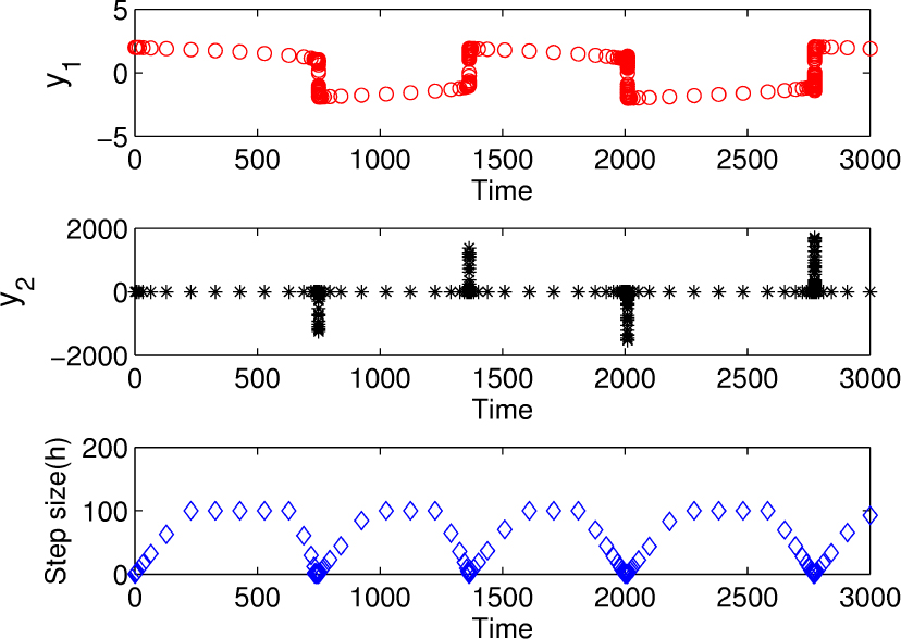
Approximated solution (y1) behavior (above), approximated solution (y2) behavior (middle) and corresponding time step size (below)
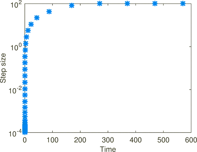
Comparison of corresponding time step size for proposed scheme and existing method (ode15s)
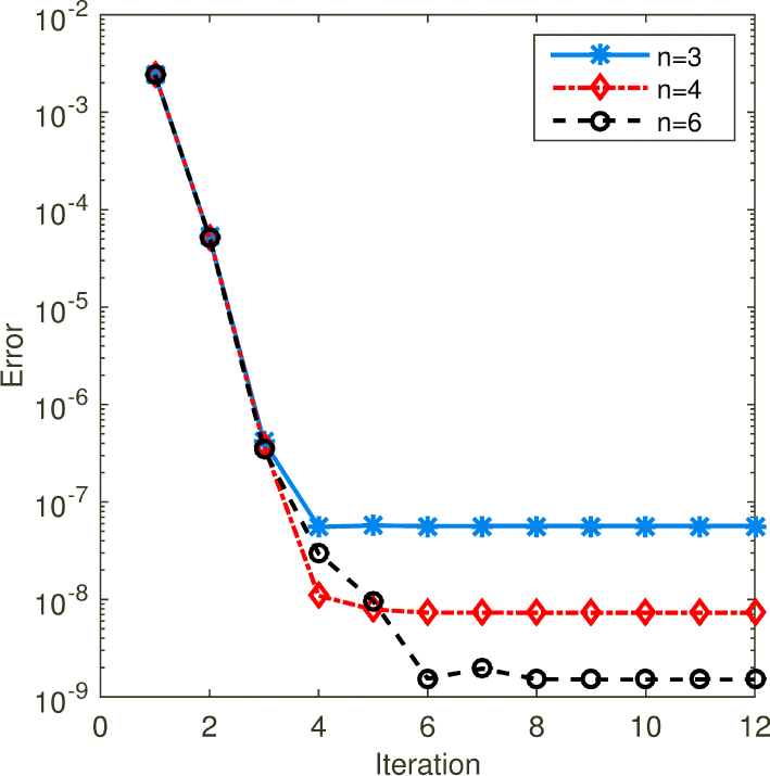
Convergence behavior of parareal algorithm with 3, 4 and 6 Radau IIa nodes
Now we apply the adaptive mesh selection strategy to the parareal algorithm with KDC as a F-propagator and BE as a G-propagator. Also, for the experiment, the KDC methods with several Radau II nodes are employed, and each parareal iteration performs the 2 outer Newton iterations for desired efficiency and the other conditions such as the tolerance for the Newton-Krylov methods or nonlinear solvers are fixed for all simulations.
Since only a few processors (less than 100) can be available in current status, we test parareal algorithm with adaptive step sizes only for non-stiff parts.
Using 72 processors, we march t = 0 to tf = 569.6 with adaptive time step size and plot the adaptive step sizes over the time domain in Fig. 5. The adaptive step size is almost same as seen in Fig. 5.
With the adaptive step size, we generate numerical results from the parareal algorithm with 3, 4 and 6 Radau II nodes for F-propagator (KDC) to examine the convergence behavior. Note that we calculate a numerical solution at time tf = 569.6 for the KDC method with 8 Radau II node and full outer Newton iterations for a reference solution, since analytic solutions of this problem are unknown.
For the experiment, we plot the error based on the reference solutions for the parareal iteration in Fig. 5. It can be seen that the accuracy of the algorithm after convergence depends on the number of Radau IIa collocation nodes in the KDC methods. Note that the KDC methods using p Radau IIa nodes is converging with an approximate order of 2p − 1 [5, 12, 13].
5 Discussion
In this paper, a numerical technique to select an adaptive step size is introduced to improve the efficiency of the parareal algorithm for stiff systems. Unlike the traditional parareal scheme, the proposed scheme allows us to use much larger time step size in non-stiff parts so that it can reduce the number of processors assigned to the corresponding interval and lead to less computational costs without any damage on accuracy.
Currently, we are working on the generalization of adaptive step size selection for any G-propagator. In particular, the proposed technique is just applicable for explicit type ODE systems, but not Differential Algebraic Equations (DAEs). In relation to this, we are constructing other parameters to measure stiffness of the given systems. At the same time, we are applying the proposed scheme to time dependent PDEs. Preliminary results are quite promising. Results along these directions will be reported soon.
Acknowledgement
This work was supported by the Hongik University new faculty research support fund.
References
[1] Butcher J. C., Order and stability of parallel methods for stiff problems: parallel methods for odes, Adv. Comput. Math., 1997, 7, 79–96.10.1023/A:1018934516771Search in Google Scholar
[2] Minion L. M., A hybrid parareal spectral deferred corrections method, Comm. in App. Math. and Comput. Sc., 2011, 5(2), 265–301.10.2140/camcos.2010.5.265Search in Google Scholar
[3] Vandewalle S., and Roose D, The parallel waveform relaxation multigrid method, in: Proceedings of the Third SIAM Conference con Parallel Processing for Sientific Computing, in: Soc. Indust. Appl. Math., 1989, 152–156.Search in Google Scholar
[4] Lions J. J., Maday Y., and Turinici G., A parareal in time discretization of PDE’s, C.R. Acad. Sci. Paris, Serie I, 2001, 332(1):16.Search in Google Scholar
[5] Bu S., and Lee J., An enhanced parareal algorithm based on the deferred correction methods for a stiff system, J. Comput. Appl. Math. 2014, 255 297–305.10.1016/j.cam.2013.05.001Search in Google Scholar
[6] Emmett M., and Minion L. M., Toward an efficient parallel in time method for partial differential equations, Comm. in App. Math. and Comput. Sc., 2012, 7(1), 105–132.10.2140/camcos.2012.7.105Search in Google Scholar
[7] Shampine F. L., Stiff and nonstiff differential equation solvers, II: Detecting stiffness with Runge-Kutta methods., ACM Trans. Math. Softw, 1977, 3(1), 44–53.10.1145/355719.355722Search in Google Scholar
[8] Staff A. G., and, Ronquist M. E., Stability of the parareal algorithm, in: Proceedings of the 15th International Domain Decomposition Conference, in: Lect. Notes Comput. Sci., 2003.Search in Google Scholar
[9] Hairer E., and Wanner G., Solving ordinary differential equations II, Springer, 1996.10.1007/978-3-642-05221-7Search in Google Scholar
[10] Bu S., Huang J., and Minion L. M., Semi-implicit Krylov deferred correction methods for differential algebraic equations, Math. Comput., 2012, 81(280) 2127–2157.10.1090/S0025-5718-2012-02564-6Search in Google Scholar
[11] Minion L. M., and Willimas S., Parareal and spectral deferred corrections, In AIP Conference Proceedings, 2008, 1048, 388–391.10.1063/1.2990941Search in Google Scholar
[12] Huang J, Jia J., and Minion L. M., Accelerating the convergence of spectral deferred correction methods, J. Comput. Phys., 2006, 214(2), 633–656.10.1016/j.jcp.2005.10.004Search in Google Scholar
[13] Huang J., Jia J., Minion L. M., Arbitrary order Krylov deferred correction methods for differential algebraic equations, J.Comput. Phys., 2007, 221,(2), 739–760.10.1016/j.jcp.2006.06.040Search in Google Scholar
© 2018 Bu, published by De Gruyter
This work is licensed under the Creative Commons Attribution-NonCommercial-NoDerivatives 4.0 License.
Articles in the same Issue
- Regular Articles
- Algebraic proofs for shallow water bi–Hamiltonian systems for three cocycle of the semi-direct product of Kac–Moody and Virasoro Lie algebras
- On a viscous two-fluid channel flow including evaporation
- Generation of pseudo-random numbers with the use of inverse chaotic transformation
- Singular Cauchy problem for the general Euler-Poisson-Darboux equation
- Ternary and n-ary f-distributive structures
- On the fine Simpson moduli spaces of 1-dimensional sheaves supported on plane quartics
- Evaluation of integrals with hypergeometric and logarithmic functions
- Bounded solutions of self-adjoint second order linear difference equations with periodic coeffients
- Oscillation of first order linear differential equations with several non-monotone delays
- Existence and regularity of mild solutions in some interpolation spaces for functional partial differential equations with nonlocal initial conditions
- The log-concavity of the q-derangement numbers of type B
- Generalized state maps and states on pseudo equality algebras
- Monotone subsequence via ultrapower
- Note on group irregularity strength of disconnected graphs
- On the security of the Courtois-Finiasz-Sendrier signature
- A further study on ordered regular equivalence relations in ordered semihypergroups
- On the structure vector field of a real hypersurface in complex quadric
- Rank relations between a {0, 1}-matrix and its complement
- Lie n superderivations and generalized Lie n superderivations of superalgebras
- Time parallelization scheme with an adaptive time step size for solving stiff initial value problems
- Stability problems and numerical integration on the Lie group SO(3) × R3 × R3
- On some fixed point results for (s, p, α)-contractive mappings in b-metric-like spaces and applications to integral equations
- On algebraic characterization of SSC of the Jahangir’s graph 𝓙n,m
- A greedy algorithm for interval greedoids
- On nonlinear evolution equation of second order in Banach spaces
- A primal-dual approach of weak vector equilibrium problems
- On new strong versions of Browder type theorems
- A Geršgorin-type eigenvalue localization set with n parameters for stochastic matrices
- Restriction conditions on PL(7, 2) codes (3 ≤ |𝓖i| ≤ 7)
- Singular integrals with variable kernel and fractional differentiation in homogeneous Morrey-Herz-type Hardy spaces with variable exponents
- Introduction to disoriented knot theory
- Restricted triangulation on circulant graphs
- Boundedness control sets for linear systems on Lie groups
- Chen’s inequalities for submanifolds in (κ, μ)-contact space form with a semi-symmetric metric connection
- Disjointed sum of products by a novel technique of orthogonalizing ORing
- A parametric linearizing approach for quadratically inequality constrained quadratic programs
- Generalizations of Steffensen’s inequality via the extension of Montgomery identity
- Vector fields satisfying the barycenter property
- On the freeness of hypersurface arrangements consisting of hyperplanes and spheres
- Biderivations of the higher rank Witt algebra without anti-symmetric condition
- Some remarks on spectra of nuclear operators
- Recursive interpolating sequences
- Involutory biquandles and singular knots and links
- Constacyclic codes over 𝔽pm[u1, u2,⋯,uk]/〈 ui2 = ui, uiuj = ujui〉
- Topological entropy for positively weak measure expansive shadowable maps
- Oscillation and non-oscillation of half-linear differential equations with coeffcients determined by functions having mean values
- On 𝓠-regular semigroups
- One kind power mean of the hybrid Gauss sums
- A reduced space branch and bound algorithm for a class of sum of ratios problems
- Some recurrence formulas for the Hermite polynomials and their squares
- A relaxed block splitting preconditioner for complex symmetric indefinite linear systems
- On f - prime radical in ordered semigroups
- Positive solutions of semipositone singular fractional differential systems with a parameter and integral boundary conditions
- Disjoint hypercyclicity equals disjoint supercyclicity for families of Taylor-type operators
- A stochastic differential game of low carbon technology sharing in collaborative innovation system of superior enterprises and inferior enterprises under uncertain environment
- Dynamic behavior analysis of a prey-predator model with ratio-dependent Monod-Haldane functional response
- The points and diameters of quantales
- Directed colimits of some flatness properties and purity of epimorphisms in S-posets
- Super (a, d)-H-antimagic labeling of subdivided graphs
- On the power sum problem of Lucas polynomials and its divisible property
- Existence of solutions for a shear thickening fluid-particle system with non-Newtonian potential
- On generalized P-reducible Finsler manifolds
- On Banach and Kuratowski Theorem, K-Lusin sets and strong sequences
- On the boundedness of square function generated by the Bessel differential operator in weighted Lebesque Lp,α spaces
- On the different kinds of separability of the space of Borel functions
- Curves in the Lorentz-Minkowski plane: elasticae, catenaries and grim-reapers
- Functional analysis method for the M/G/1 queueing model with single working vacation
- Existence of asymptotically periodic solutions for semilinear evolution equations with nonlocal initial conditions
- The existence of solutions to certain type of nonlinear difference-differential equations
- Domination in 4-regular Knödel graphs
- Stepanov-like pseudo almost periodic functions on time scales and applications to dynamic equations with delay
- Algebras of right ample semigroups
- Random attractors for stochastic retarded reaction-diffusion equations with multiplicative white noise on unbounded domains
- Nontrivial periodic solutions to delay difference equations via Morse theory
- A note on the three-way generalization of the Jordan canonical form
- On some varieties of ai-semirings satisfying xp+1 ≈ x
- Abstract-valued Orlicz spaces of range-varying type
- On the recursive properties of one kind hybrid power mean involving two-term exponential sums and Gauss sums
- Arithmetic of generalized Dedekind sums and their modularity
- Multipreconditioned GMRES for simulating stochastic automata networks
- Regularization and error estimates for an inverse heat problem under the conformable derivative
- Transitivity of the εm-relation on (m-idempotent) hyperrings
- Learning Bayesian networks based on bi-velocity discrete particle swarm optimization with mutation operator
- Simultaneous prediction in the generalized linear model
- Two asymptotic expansions for gamma function developed by Windschitl’s formula
- State maps on semihoops
- 𝓜𝓝-convergence and lim-inf𝓜-convergence in partially ordered sets
- Stability and convergence of a local discontinuous Galerkin finite element method for the general Lax equation
- New topology in residuated lattices
- Optimality and duality in set-valued optimization utilizing limit sets
- An improved Schwarz Lemma at the boundary
- Initial layer problem of the Boussinesq system for Rayleigh-Bénard convection with infinite Prandtl number limit
- Toeplitz matrices whose elements are coefficients of Bazilevič functions
- Epi-mild normality
- Nonlinear elastic beam problems with the parameter near resonance
- Orlicz difference bodies
- The Picard group of Brauer-Severi varieties
- Galoisian and qualitative approaches to linear Polyanin-Zaitsev vector fields
- Weak group inverse
- Infinite growth of solutions of second order complex differential equation
- Semi-Hurewicz-Type properties in ditopological texture spaces
- Chaos and bifurcation in the controlled chaotic system
- Translatability and translatable semigroups
- Sharp bounds for partition dimension of generalized Möbius ladders
- Uniqueness theorems for L-functions in the extended Selberg class
- An effective algorithm for globally solving quadratic programs using parametric linearization technique
- Bounds of Strong EMT Strength for certain Subdivision of Star and Bistar
- On categorical aspects of S -quantales
- On the algebraicity of coefficients of half-integral weight mock modular forms
- Dunkl analogue of Szász-mirakjan operators of blending type
- Majorization, “useful” Csiszár divergence and “useful” Zipf-Mandelbrot law
- Global stability of a distributed delayed viral model with general incidence rate
- Analyzing a generalized pest-natural enemy model with nonlinear impulsive control
- Boundary value problems of a discrete generalized beam equation via variational methods
- Common fixed point theorem of six self-mappings in Menger spaces using (CLRST) property
- Periodic and subharmonic solutions for a 2nth-order p-Laplacian difference equation containing both advances and retardations
- Spectrum of free-form Sudoku graphs
- Regularity of fuzzy convergence spaces
- The well-posedness of solution to a compressible non-Newtonian fluid with self-gravitational potential
- On further refinements for Young inequalities
- Pretty good state transfer on 1-sum of star graphs
- On a conjecture about generalized Q-recurrence
- Univariate approximating schemes and their non-tensor product generalization
- Multi-term fractional differential equations with nonlocal boundary conditions
- Homoclinic and heteroclinic solutions to a hepatitis C evolution model
- Regularity of one-sided multilinear fractional maximal functions
- Galois connections between sets of paths and closure operators in simple graphs
- KGSA: A Gravitational Search Algorithm for Multimodal Optimization based on K-Means Niching Technique and a Novel Elitism Strategy
- θ-type Calderón-Zygmund Operators and Commutators in Variable Exponents Herz space
- An integral that counts the zeros of a function
- On rough sets induced by fuzzy relations approach in semigroups
- Computational uncertainty quantification for random non-autonomous second order linear differential equations via adapted gPC: a comparative case study with random Fröbenius method and Monte Carlo simulation
- The fourth order strongly noncanonical operators
- Topical Issue on Cyber-security Mathematics
- Review of Cryptographic Schemes applied to Remote Electronic Voting systems: remaining challenges and the upcoming post-quantum paradigm
- Linearity in decimation-based generators: an improved cryptanalysis on the shrinking generator
- On dynamic network security: A random decentering algorithm on graphs