
Curves in the Lorentz-Minkowski plane: elasticae, catenaries and grim-reapers
-
Ildefonso Castro
 ,
Ildefonso Castro-Infantes
,
Ildefonso Castro-Infantes

Abstract
This article is motivated by a problem posed by David A. Singer in 1999 and by the classical Euler elastic curves. We study spacelike and timelike curves in the Lorentz-Minkowski plane 𝕃2 whose curvature is expressed in terms of the Lorentzian pseudodistance to fixed geodesics. In this way, we get a complete description of all the elastic curves in 𝕃2 and provide the Lorentzian versions of catenaries and grim-reaper curves. We show several uniqueness results for them in terms of their geometric linear momentum. In addition, we are able to get arc-length parametrizations of all the aforementioned curves and they are depicted graphically.
1 Introduction
The motivation of this article is the following problem posed by David A. Singer in [1]:
Can a plane curve be determined if its curvature is given in terms of its position?
Probably, the most interesting solution to this question corresponds to the classical Euler elastic curves (cf. [2] for instance), whose curvature is proportional to one of the coordinate functions. Singer himself proved (see Theorem 3.1 in [1]) that the problem of determining a curve α whose curvature is κ(r), where r is the distance from the origin, is solvable by quadratures when rκ(r) is a continuous function. But even the simple case κ(r) = r studied in [1], where elliptic integrals appear, illustrated the following fact: although the corresponding differential equation is integrable by quadratures, it does not imply that the integrations are easy to perform. There are many interesting papers devoted to studying particular cases on the proposed problem of determining α = (x, y) given κ = κ(r): for example [3, 4, 5, 6, 7, 8, 9]. In addition, the authors studied recently the cases κ = κ(y) and κ = κ(r) in [10] and [11] respectively, for a large number of prescribed curvature functions.
The aim of this paper is the study of Singer’s problem in the Lorentz-Minkowski plane; that is, to try to determine those curves γ = (x, y) in 𝕃2 whose curvature κ depends on some given function κ = κ(x, y). We must focus on spacelike and timelike curves, since the curvature κ is in general not well defined on lightlike points, and because lightlike curves in 𝕃2 are segments parallel to the straight lines determining the light cone. When the ambient space is 𝕃2, our knowledge is more restricted in comparison with the Euclidean case. Even though the fundamental existence and uniqueness theorem, which states that a spacelike or timelike curve is uniquely determined (up to Lorentzian transformations) by its curvature given as a function of its arc-length, is still valid. Eventually, it is very difficult to find the curve explicitly in practice and most cases become elusive. In fact, we can only mention the articles [12, 13] in this line, both devoted to Sturmian spiral curves. We should remark that although some families of space curves in the Lorentz-Minkowski space 𝕃3 (helices, Bertrand and Mannheim curves) are well studied as in Euclidean case, the papers in the pseudo-Euclidean plane are limited, to our knowledge (see [14, 15] for example).
From a geometric-analytic point of view, we deal with the following case of Singer’s problem in the Lorentzian setting (see Section 2 for details): For a unit speed parametrization of a spacelike or timelike curve γ = (x, y) in 𝕃2, we prescribe its curvature with the analytic extrinsic condition κ = κ(y) or κ = κ(x). Obviously, if one writes the curve γ as the graphs x = f(y) or y = f(x) locally, the above condition is satisfied. But we aim to study the problem from a different point of view: We offer a geometric interpretation of these conditions on κ in terms of the Lorentzian pseudodistance to spacelike or timelike fixed geodesics, and would like to determine the analytic representation of the arc-length parametrization γ (s) explicitly and, consequently, its intrinsic equation κ = κ(s).
Singer’s proof of the aforementioned Theorem 3.1 in [1] is based on giving such a curvature κ = κ(r) an interpretation of a central potential in the plane and finding the trajectories by the standard methods in classical mechanics. On the other hand, since the curvature κ may be also interpreted as the tension that γ receives at each point as a consequence of the way it is immersed in 𝕃2, we make use of the notion of geometric linear momentum of γ when κ = κ(y) or κ = κ(x) in order to get two abstract integrability results (Theorems 2.1 and 2.6) in the same spirit of Theorem 3.1 in [1]. We show that the problem of determining such a curve is solvable by three quadratures if κ = κ(y) or κ = κ(x) is a continuous function. In addition, the geometric linear momentum turns to be a primitive function of the curvature and determines uniquely such a curve (up to translations in x-direction or in y-direction respectively). In general, one finds great difficulties (see Remark 2.5) in carrying out the computations in most cases. Hence we focus on finding interesting curves for which the required computations can be achieved explicitly, in terms of standard functions, and we pay attention to identifying, computing and plotting such examples.
In this way, we are first successful in the complete description of all the spacelike and timelike elastic curves in the Lorentz-Minkowski plane. Elastic curves in Euclidean plane were already classified by Euler in 1743. The classification problem of elastic curves and its generalizations in real space forms has been considered through different approaches (see [16, 17, 18, 19, 20], etc.) But in 𝕃2 only the elastic Sturmian spirals recently studied in [13] were known to us. In Section 3, we characterize most of the spacelike and timelike elastic curves in 𝕃2 —according to Singer’s problem— by the condition κ(y) = 2λy + μ, λ > 0, μ ∈ ℝ, and this allows us their explicit description by arc-length parametrizations in terms of Jacobi elliptic functions.
Moreover, we find out the Lorentzian versions of some interesting classical curves in the Euclidean context. Specifically, we study the generatrix curves of the maximal catenoids of the first and the second kind described in [21] in Section 4, which we will call Lorentzian catenaries. We also consider curves that satisfy a translating-type soliton equation in Section 5, which we will call Lorentzian grim-reapers (see [22]). We provide uniqueness results for both of them in terms of their geometric linear momentum (Corollaries 4.1, 5.1, 6.1, 6.2 and 6.3). We also generalize them by describing all the spacelike and timelike curves in 𝕃2 whose curvature satisfies κ(y) = λ /y2, λ > 0, and κ(y) = λey, λ > 0.
In [23], we afford two other cases of Singer’s problem in the Lorentz-Minkowski plane: the spacelike and timelike curves in 𝕃2 whose curvature depends on the Lorentzian pseudodistance from the origin, and those ones whose curvature depends on the Lorentzian pseudodistance through the horizontal or vertical geodesic to a fixed lightlike geodesic.
2 Spacelike and timelike curves in Lorentz-Minkowski plane
We denote by 𝕃2 := (ℝ2, g = −dx2 + dy2) the Lorentz-Minkowski plane, where (x, y) are the rectangular coordinates on 𝕃2. We say that a non-zero vector v ∈ 𝕃2 is spacelike if g(v, v) > 0, lightlike if g(v, v) = 0, and timelike if g(v, v) < 0.
Let γ = (x, y): I ⊆ ℝ → ℝ2 be a curve. We say that γ = γ(t) is spacelike (resp. timelike) if the tangent vector γ′(t) is spacelike (resp. timelike) for all t ∈ I. A point γ (t) is called a lightlike point if γ′(t) is a lightlike vector. We study geometric properties of curves that have no lightlike points in this section, because the curvature is not in general well defined at the lightlike points.
Hence, let γ = (x, y) be a spacelike (resp. timelike) curve parametrized by arc-length; that is, g(γ̇(s), γ̇(s)) = 1 (resp. g(γ̇(s), γ̇(s)) = −1) ∀ s ∈ I, where I is some interval in ℝ. Here ˙ means derivation with respect to s. We will say that γ = γ(s) is a unit-speed curve in both cases.
We define the Frenet dihedron in such a way that the curvature κ has a sign and then it is only preserved by direct rigid motions (see [14]): Let T = γ̇ = (ẋ, ẏ) be the tangent vector to the curve γ and we choose N = γ̇⊥ = (ẏ, ẋ) as the corresponding normal vector. We remark that T and N have different causal character. Let g(T, T) = ϵ, with ϵ = 1 if γ is spacelike, and ϵ = −1 if γ is timelike. Then g(N, N) = −ϵ. The (signed) curvature of γ is the function κ = κ(s) such that
where
The Frenet equations of γ are given by (1) and
It is possible, as it happens in the Euclidean case, to obtain a parametrization by arc-length of the curve γ in terms of integrals of the curvature. Specifically, any spacelike curve α (s) in 𝕃2 can be represented by
and any timelike curve β (s) in 𝕃2 can be represented by
For example, up to a translation, any spacelike geodesic can be written as
and any timelike geodesic can be written as
On the other hand, the transformation Rν : 𝕃2 → 𝕃2, ν ∈ ℝ, given by
is an isometry of 𝕃2 that preserves the curvature of a curve γ and satisfies
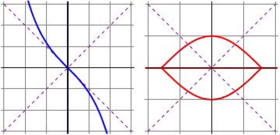
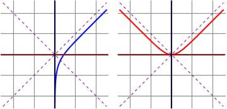
In this way, any spacelike geodesic is congruent to α0, i.e. the y-axis, and any timelike geodesic is congruent to β0, i.e. the x-axis (see Figure 1).
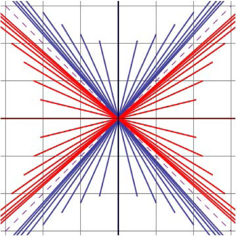
Spacelike (blue) and timelike (red) geodesics in 𝕃2.
2.1 Curves in 𝕃2 such that κ = κ(y)
Given a spacelike or timelike curve γ = (x, y) in 𝕃2, we are first interested in the analytical condition κ = κ(y). We look for its geometric interpretation. For this purpose, we define the Lorentzian pseudodistance by
We fix the timelike geodesic β0, i.e. the x-axis. Given an arbitrary point P = (x, y) ∈ 𝕃2, y ≠ 0, we consider all the spacelike geodesics αm with slope m = coth φ0, |m| > 1, passing through P, and let P′ = (x − y/m, 0) the crossing point of αm and the x-axis (see Figure 2). Then:
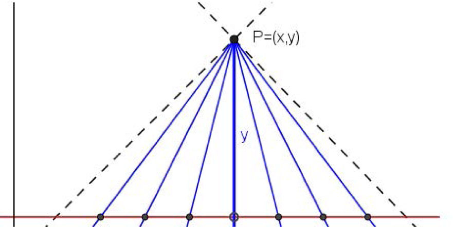
Spacelike geodesics in 𝕃2 passing through P.
and the equality holds if and only if φ0 = 0, that is, αm is a vertical geodesic. Thus |y| is the maximum Lorentzian pseudodistance through spacelike geodesics from P = (x, y) ∈ 𝕃2, y ≠ 0, to the timelike geodesic given by the x-axis.
At a given point γ(s) = (x(s), y(s)) on the curve, the geometric linear momentum (with respect to thex-axis) 𝓚 is given by
In physical terms, using Noether’s Theorem, 𝓚 may be interpreted as the linear momentum with respect to the x-axis of a particle of unit mass with unit-speed and trajectory γ.
Given that γ is unit-speed, that is, −ẋ2 + ẏ2 = ϵ, and (8), we easily obtain that
Thus, given 𝓚 = 𝓚(y) as an explicit function, looking at (9) one may attempt to compute y(s) and x(s) in three steps: integrate to get s = s(y), invert to get y = y(s) and integrate to get x = x(s).
In addition, we have that the curvature κ satisfies (1) and (3), i.e. ẍ = κẏ. Taking into account (8), we deduce that
that is, 𝓚 = 𝓚(y) can be interpreted as an anti-derivative of κ(y).
As a summary, we have proved the following result in the spirit of Theorem 3.1 in [1].
Theorem 2.1
Letκ = κ(y) be a continuous function. Then the problem of determining locally a spacelike or timelike curve in 𝕃2whose curvature isκ(y) with geometric linear momentum 𝓚 (y) satisfying(10) —|y| being the (non constant) maximum Lorentzian pseudodistance through spacelike geodesics to thex-axis— is solvable by quadratures considering the unit speed curve (x(s), y(s)), wherey(s) andx (s) are obtained through (9) after invertings = s(y). Such a curve is uniquely determined by 𝓚 (y) up to a translation in thex-direction (and a translation of the arc parameters).
Remark 2.2
If we prescribeκ = κ(y), the method described in Theorem 2.1 clearly implies the computation of three quadratures, following the sequence:
Anti-derivative ofκ(y):
Arc-length parametersof (x(s), y(s)) in terms ofy:
where 𝓚 (y)2 + ϵ > 0, and invertings = s(y) to gety = y(s).
First coordinate of (x(s), y(s)) in terms ofs:
We note that we get a one-parameter family of curves in 𝕃2satisfyingκ = κ(y) according to the geometric linear momentum chosen in (i). It will distinguish geometrically the curves inside the same family by their relative position with respect to thex-axis. We remark that we can recoverκfrom 𝓚 simply by means ofκ(y) = d𝓚/dy.
We show two illustrative examples applying steps (i)-(iii) in Remark 2.2:
Example 2.3
(κ ≡ 0). Then 𝓚 ≡ c ∈ ℝ,
Example 2.4
(κ ≡ k0 > 0). Now 𝓚 (y) = k0y + c, c ∈ ℝ. Thus
Spacelike (blue) and timelike (red) pseudocircles in 𝕃2 with constant positive curvature.
Remark 2.5
The main difficulties one can find carrying on the strategy described in Theorem 2.1 (or in Remark 2.2) to determine a curve (x, y) in 𝕃2whose curvature isκ = κ(y) are the following:
The previous integration gives uss = s(y); it is not always possible to obtain explicitlyy = y(s), what is necessary to determine the curve.
Even knowing explicitlyy = y(s), the integration to getx (s) may be impossible to perform using elementary or known functions.
2.2 Curves in 𝕃2 such that κ = κ(x)
Given a spacelike or timelike curve γ = (x, y) in 𝕃2, we are now interested in the analytical condition κ = κ(x) and we search for its geometric interpretation using again the Lorentzian pseudodistance δ. We fix the spacelike geodesic α0, i.e. the y-axis. Given an arbitrary point P = (x, y) ∈ 𝕃2, x ≠ 0, we consider all the timelike geodesics βm with slope m = tanh ϕ0, |m| < 1, passing through P, and let P′ = (0, y − mx) the crossing point of βm and the y-axis (see Figure 4). Then:

Timelike geodesics in 𝕃2 passing through P.
and the equality holds if and only if ϕ0 = 0, that is, βm is a horizontal geodesic. Thus |x| is now the maximum Lorentzian pseudodistance through timelike geodesics from P = (x, y) ∈ 𝕃2, x ≠ 0, to the spacelike geodesic given by the y-axis.
We now make a similar study to the one made in the preceding section. At a given point γ (s) = (x(s), y(s)) on the curve, the geometric linear momentum (respect to they-axis) 𝓚 is given by
In physical terms, using Noether’s Theorem, 𝓚 may be interpreted as the linear momentum with respect to the y-axis of a particle of unit mass with unit-speed and trajectory γ.
Using that γ is unit-speed, that is, −ẋ2 + ẏ2 = ϵ, and (11), we easily obtain that
Thus, given 𝓚 = 𝓚 (x) as an explicit function, looking at (12) one may attempt to compute x(s) and y(s) in three steps: integrate to get s = s(x), invert to get x = x(s) and integrate to get y = y(s).
In addition, we have that the curvature κ satisfies (1) and (3), i.e. ÿ = κ ẋ. Taking into account (11), we deduce that
that is, 𝓚 = 𝓚(x) can be interpreted as an anti-derivative of κ(x).
As a summary, we have proved the following result, dual in a certain sense to Theorem 2.1
Theorem 2.6
Letκ = κ(x) be a continuous function. Then the problem of determining locally a spacelike or timelike curve in 𝕃2whose curvature isκ(x) with geometric linear momentum 𝓚 (x) satisfying(13) —|x| being the (non constant) maximum Lorentzian pseudodistance through timelike geodesics to they-axis— is solvable by quadratures considering the unit speed curve (x(s), y(s)), wherex(s) andy(s) are obtained through (12) after invertings = s(x). Such a curve is uniquely determined by 𝓚 (x) up to a translation in they-direction (and a translation of the arc parameters).
Remark 2.7
The duality between Theorems 2.1 and 2.6 is explained thanks to the following observation: Ifγ = (x, y) is a spacelike (resp. timelike) curve in 𝕃2such thatκ = κ(y), thenγ̂ = (y, x) is a timelike (resp. spacelike) curve in 𝕃2such thatκ = κ(x).
3 Elastic curves in the Lorentz-Minkowski plane
A unit speed spacelike or timelike curve γ in 𝕃2 is said to be an elastica under tensionσ (see [25]) if it satisfies the differential equation
for some value of σ ∈ ℝ. They are critical points of the elastic energy functional ∫γ(κ2 + σ )ds acting on curves in 𝕃2 with suitable boundary conditions. If σ = 0, then γ is called a free elastica. The possible constant solutions of (14) are the trivial solution κ ≡ 0 and κ ≡
Multiplying (14) by 2κ̇ and integration allow us to introduce the energyE ∈ ℝ of an elastica:
If E = σ2/4, (15) reduces to κ̇2 = (κ2/2 + σ/2)2, whose solutions are given by
Special elastic curves σ = 1, 0, −1 (blue, spacelike; red, timelike).
In this section we will study those spacelike and timelike curves in 𝕃2 satisfying
and we will show its close relationship with the elastic curves of 𝕃2. Following Theorem 2.1, we must consider the geometric linear momentum 𝓚(y) = ay2 + by + c, c ∈ ℝ. In the following result, we show that we are studying precisely elastic curves.
Proposition 3.1
Letγbe a spacelike or timelike curve in 𝕃2.
If the curvature ofγis given by(16)with geometric linear momentum 𝓚(y) = ay2 + by + c, a ≠ 0, b, c ∈ ℝ, thenγis an elastica under tensionσ = 4 ac − b2and energyE = 4ϵa2 + σ2/4 (whereϵ = 1 ifγis spacelike andϵ = −1 ifγis timelike).
Ifγis an elastica under tensionσand energyE, with E ≠ σ2/4, then the curvature ofγis given by(16).
Proof
Without restriction we can consider γ parametrized by arc-length. Assume first that 𝓚(y) = ay2 + by + c, a ≠ 0, b, c ∈ ℝ. In order γ to be an elastica, we must check that κ given by (16) satisfies (14) or (15). We have that κ̇2 = 4a2ẏ2 and (9) implies that ẏ2 = 𝓚 2 + ϵ = (ay2 + bc + c)2 + ϵ. By substituting y = (κ − b)/2a, it is a long exercise to check (15) taking σ = 4ac − b2 and E = 4ϵa2 + σ2/4. We observe that E − σ2/4 ≠ 0.
Conversely, assume that γ is an elastica under tension σ and energy E. We write locally γ as a graph x = x(y) and then κ = κ(y) obviously. Using Theorem 2.1, κ̇2 = κ′(y)2ẏ2 = 𝓚″(y)2(𝓚(y)2 + ϵ). Then (15) translates into
If E ≠ σ2/4, we can define
Given γ = (x, y) satisfying (16) with a > 0 without restriction, we take γ̂ =
The trivial solution κ ≡ 0 to (14) corresponds in (18) to the x-axis y ≡ 0.
Following the strategy described in Remark 2.2, we can control the spacelike or timelike curves (x(s),y(s)) in 𝕃2 satisfying (18) with geometric linear momentum 𝓚(y) = y2 + c, c ∈ ℝ, by means of
and
with c ∈ ℝ. The integrations of (19) and (20) involve Jacobi elliptic functions and elliptic integrals.
3.1 Spacelike elastic curves in the Lorentz-Minkowski plane
We take ϵ = 1 and put c = sinh η, η ∈ ℝ. Then these spacelike elastic curves will have energy E = 4cosh2η (see Proposition 3.1). Now (19) is rewritten as
After a long computation, using formulas 225.00 and 129.04 of [24] and abbreviating cη := cosh η, we finally get that
with s ∈ (2mK(kη)/
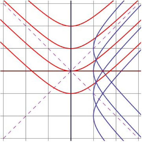
where sη := sinh η and cn(⋅, kη), sd(⋅, kη) and ds(⋅, kη) are Jacobian elliptic functions and E(⋅, kη) denotes the elliptic integral of the second kind of modulus kη (see [24]). We remark that, using (18), the intrinsic equations of the curves αη = (xη, yη), η ∈ ℝ (see Figure 6), are given by
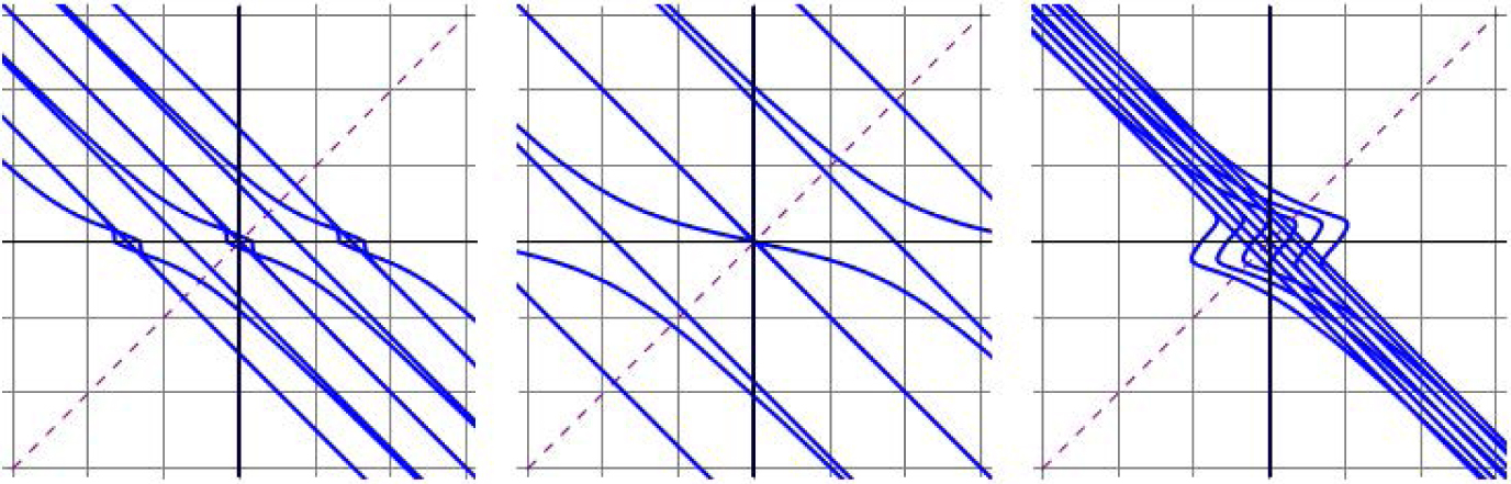
Spacelike elastic curves αη (η = 0, 1.5, −1.5).
3.2 Timelike elastic curves in the Lorentz-Minkowski plane
When we take ϵ = −1 in (19), we have that
and then we must distinguish five cases:
c = 1, i.e. 𝓚 (y) = y2 + 1.
c = −1, i.e. 𝓚 (y) = y2 − 1.
c > 1; put c := cosh2δ, δ > 0, and so 𝓚 (y) = y2 + cosh2δ.
|c| < 1: put c := sin ψ, −π/2 < ψ < π/2, and so 𝓚 (y) = y2 + sin ψ.
c < −1: put c := −cosh2τ, τ > 0, and so 𝓚 (y) = y2 − cosh2τ.
3.2.1 Timelike elastic curves in 𝕃2 with 𝓚 (y) = y2± 1
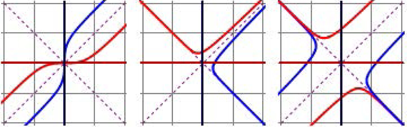
In these cases, (24) becomes elementary and both of them produce timelike elastic curves with null energy (see Proposition 3.1). A straightforward computation, using (24) and (20), provides us the only (up to translations in the x-direction) timelike elastic curve (x1(s)), y1(s) with geometric linear momentum 𝓚 (y) = y2 + 1 (see Figure 7, left), given by
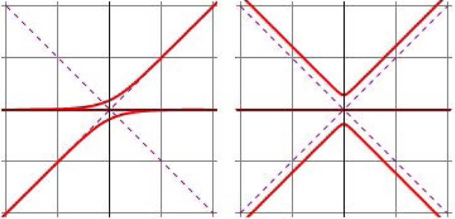
Timelike elastic curves with 𝓚 (y) = y2± 1.
and the only (up to translations in the x-direction) timelike elastic curve (x−1(s)), y−1(s) with geometric linear momentum 𝓚 (y) = y2 −1 (see Figure 7, right), given by
Using (18), the intrinsic equations of these curves are given by
respectively.
3.2.2 Timelike elastic curves in 𝕃2 with 𝓚 (y) = y2 + cosh2δ, δ > 0
Since c = cosh2δ in this case, these timelike elastic curves will have energy E = 4sinh2δ(cosh2δ + 1) > 0 (see Proposition 3.1) and we can write (24) simply as
Using formula 221.00 of [24] and abbreviating cδ := cosh δ and sδ := sinh δ, we obtain that
with s ∈ ((2m − 1) K(kδ)/
where dn(⋅, kδ) is a Jacobian elliptic function and E(⋅, kδ) denotes the elliptic integral of the second kind of modulus kδ (see [24]). We point out that, using (18), the intrinsic equations of the curves βδ = (xδ, yδ), δ > 0 (see Figure 8), are given by
Timelike elastic curves βδ (δ = 0.5, 1, 1.5).
3.2.3 Timelike elastic curves in 𝕃2 with 𝓚 (y) = y2 + sin ψ, |ψ| < π/2
As c = sin ψ in this case, these timelike elastic curves will have energy E = −4cos2ψ < 0 (see Proposition 3.1) and (24) can be written as
Using formula 211.00 of [24] and abbreviating sψ := sin ψ, we deduce that
with s ∈ ((2m − 1) K(kψ)/
where dn(⋅, kψ) and tn(⋅, kψ) are Jacobian elliptic function and E(⋅, kψ) denotes the elliptic integral of the second kind of modulus kψ (see [24]). We point out that, using (18), the intrinsic equations of the curves βψ = (xψ, yψ), |ψ| < π/2 (see Figure 9), are given by

Timelike elastic curves βψ (ψ = −π/4, 0, π/6).
3.2.4 Timelike elastic curves in 𝕃2 with 𝓚 (y) = y2 − cosh2τ, τ > 0
When c = −cosh2τ, these timelike elastic curves will have energy E = 4sinh2τ(cosh2τ + 1) > 0 (see Proposition 3.1) and we can write (24) simply as
Using formula 216.00 of [24] and abbreviating cτ := cosh τ, after a long straightforward computation we arrive at
with s ∈ ((2m − 1) K(kτ)/
where dn(⋅, kτ) and tn(⋅, kτ) are Jacobian elliptic function and E(⋅, kτ) denotes the elliptic integral of the second kind of modulus kτ (see [24]). We point out that, using (18), the intrinsic equations of the curves βτ = (xτ, yτ), τ > 0 (see Figure 10), are given by
Timelike elastic curves βτ (τ = 1, 2, 3).
4 Curves in 𝕃2 such that κ(y) = λ/y2, λ > 0
In this section we will study those spacelike and timelike curves in 𝕃2 satisfying
and we will show that some of them can be considered as Lorentzian versions of catenaries in 𝕃2 (see Section 4 in [10]). Given γ = (x, y) satisfying (34), if we take
with y ≠ 0. Following Theorem 2.1, we must consider the geometric linear momentum 𝓚(y) = c − 1/y, c ∈ ℝ.
4.1 Case 𝓚(y) = −1/y. Lorentzian catenaries
We follow the steps described in Remark 2.2 and so
Then s2 = 1 + ϵy2, and hence
Consequently, recalling that 𝓚(y) = −1/y, we get:
We arrive at the graphs y = − sinh x, x ∈ ℝ, at the spacelike case ϵ = 1, and y = ± cos x, |x| < π/2, at the timelike case ϵ = −1 (see Figure 11). Using (35), their intrinsic equations are given by
Curves with 𝓚(y) = −1/y; spacelike (left), timelike (right).
On the other hand, Kobayashi introduced in [21], by studying maximal rotation surfaces in 𝕃3 := (ℝ3, −dx2 + dy2 + dz2), a couple of catenoids. Specifically, Example 2.5 in [21] presents (up to dilations) the catenoid of the first kind by the equation y2 + z2 − sinh2x = 0 and we can deduce the equation x2 − z2 = cos2y for the catenoid of the second kind given (up to dilations) in Example 2.6 in [21] (see Figure 12).
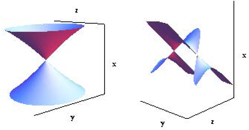
Catenoid of the first kind (left) and the second kind (right) in 𝕃3.
The generatrix curves (in a certain sense) of both catenoids will be referred as Lorentzian catenaries. Specifically, we call the graph y = − sinh x, x ∈ ℝ, the Lorentzian catenary of the first kind, and the bigraph x = ± cos y, |y| < π/2, the Lorentzian catenary of the second kind. As a summary of this section, taking into account Remark 2.7, we conclude with the following geometric characterization of them.
Corollary 4.1
The Lorentzian catenary of the first kindy = − sinh x, x ∈ ℝ, is the only spacelike curve (up to translations in thex-direction) in 𝕃2with geometric linear momentum 𝓚(y) = −1/y.
The Lorentzian catenary of the second kindx = ± cos y, |y| < π/2, is the only spacelike curve (up to translations in they-direction) in 𝕃2with geometric linear momentum 𝓚 (x) = −1/x.
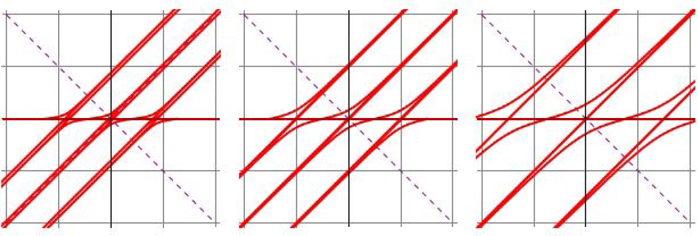
4.2 Case 𝓚(y) = c − 1/y, c ≠ 0
When c ≠ 0, it is difficult to get the arc parameter s as a function of y; however, we can eliminate ds using parts (ii) and (iii) in Remark 2.2, obtaining
If c = 0, we easily recover the Lorentzian catenaries studied in the previous section. If c ≠ 0, we distinguish the following cases according to the expression of polynomial P(y):
Spacelike case (ϵ = 1), 𝓚(y) = c − 1/y:
We notice that if c = 0 above, we recover x = −arcsinh y (see Figure 13).
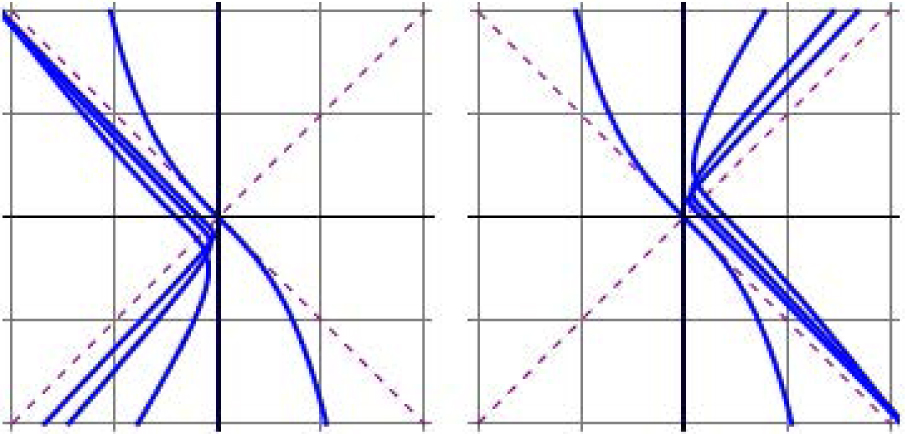 Fig. 13
Curves with 𝓚(y) = c − 1/y; spacelike c ≤ 0 (left), spacelike c ≥ 0 (right).
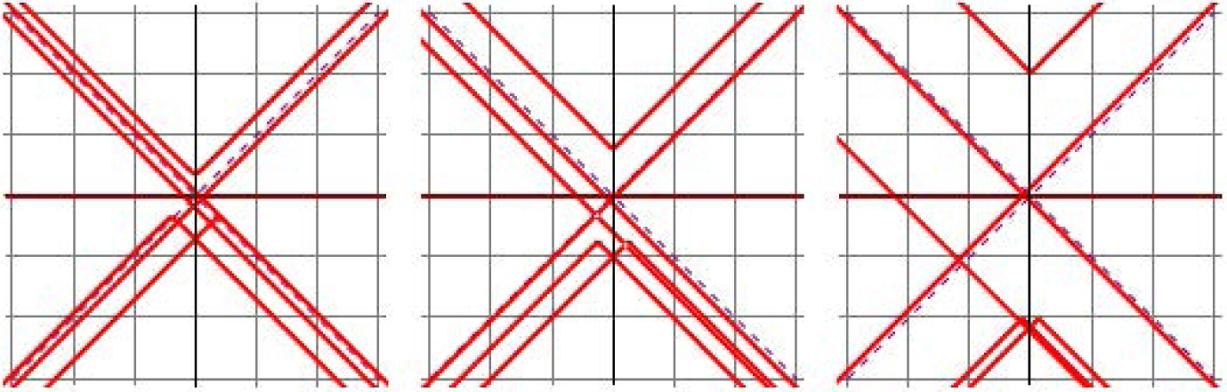
Timelike case (ϵ = −1):
𝓚(y) = 1 − 1/y (see Figure 14):
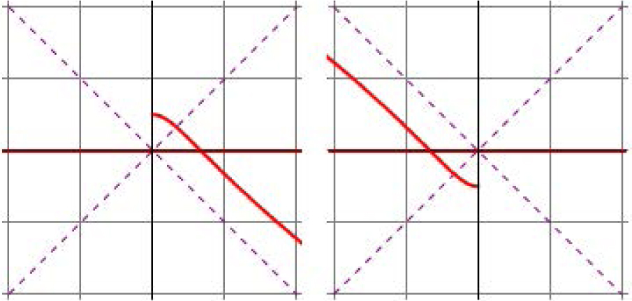 Fig. 14
Timelike curves with 𝓚(y) = 1 − 1/y (left) and 𝓚(y) = − 1 − 1/y (right).
𝓚(y) = − 1 − 1/y (see Figure 14):
𝓚(y) = c − 1/y, |c| > 1:
𝓚(y) = c − 1/y, |c| < 1:
5 Curves in 𝕃2 such that κ(y) = λ ey, λ > 0
In this section we will study those spacelike and timelike curves in 𝕃2 satisfying
and we will introduce what can be considered the Lorentzian versions of grim-reaper curves in 𝕃2 (see Section 7 in [10]). Given γ = (x, y) satisfying (36), if we take γ̂ = (x, y + log λ) then, up to a translation, we can only consider the condition
Following Theorem 2.1, we deal with the geometric linear momentum 𝓚(y) = ey + c, c ∈ ℝ.
5.1 Case 𝓚(y) = ey. Lorentzian grim-reapers
Following the steps in Remark 2.2, putting u = ey, we have that
Hence:
Consequently, recalling that 𝓚(y) = ey, we obtain:
A straightforward computation leads us to the graphs y = log (sinh x), x > 0, at the spacelike case ϵ = 1, and y = log (cosh x), x ∈ ℝ, at the timelike case ϵ = −1 (see Figure 15). Using (37), their intrinsic equations are given by κ(s) = − csch s, s < 0, and κ(s) = sec s, |s| < π/2, respectively.
Curves with 𝓚(y) = ey; spacelike (left), timelike (right).
It is straightforward to check that both curves satisfy the translating-type soliton equation κ = g ((0, 1), N). Hence we have obtained in this section (see also Section 7.1 in [10]) Lorentzian versions of the grim-reaper curves of Euclidean plane. We will simply call them Lorentzian grim-reapers. As a summary, we conclude with the following geometric characterization of them.
Corollary 5.1
The Lorentzian grim-reapery = log (sinh x), x > 0, is the only spacelike curve (up to translations in thex-direction) in 𝕃2with geometric linear momentum 𝓚(y) = ey.
The Lorentzian grim-reapery = log (cosh x), x ∈ ℝ, is the only timelike curve (up to translations in thex-direction) in 𝕃2with geometric linear momentum 𝓚(y) = ey.
5.2 Case 𝓚(y) = ey + c, c ≠ 0
When c ≠ 0, it is longer and more difficult to get the arc parameter s as a function of y; however, we can eliminate ds using parts (ii) and (iii) in Remark 2.2. Putting u = ey, we obtain:
If c = 0, we recover the Lorentzian grim-reaper curves studied in the previous section. If c ≠ 0, we distinguish the following cases according to the expression of polynomial P(u):
Spacelike case (ϵ = 1), 𝓚(y) = ey + c:
We notice that if c = 0 above, we recover the graph y = log (sinh x) (see Figure 16).
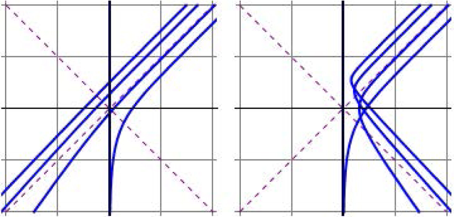 Fig. 16
Curves with 𝓚(y) = ey + c; spacelike c ≤ 0 (left), spacelike c ≥ 0 (right).
Timelike case (ϵ = −1):
𝓚(y) = ey + 1: (see Figure 17)
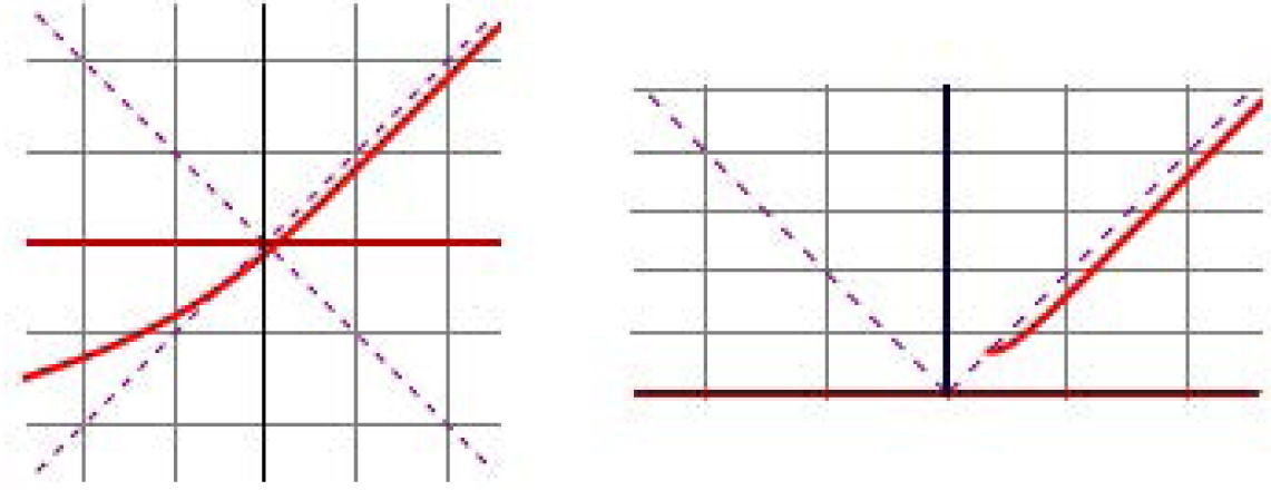 Fig. 17
Timelike curves with 𝓚(y) = ey + 1 (left) and 𝓚(y) = ey − 1 (right).
𝓚(y) = ey − 1: (see Figure 17):
𝓚(y) = ey + c, |c| > 1:
𝓚(y) = ey + c, |c| < 1:
6 Other integrable curves in 𝕃2
The aim of this section is to collect some interesting curves in 𝕃2 that can be easily determined by their geometric linear momentum, following the strategy described in Theorem 2.1 and Remark 2.2.
6.1 Timelike curves in 𝕃2 such that κ(y) = csch2y
In this case, being y ≠ 0, we only consider the geometric linear momentum 𝓚 (y) = −coth y. Then:
Thus:
and
We arrive at the graph x = −sinh y, y ∈ ℝ, whose intrinsic equation is (using that κ(y) = csch2y) given by
Corollary 6.1
The Lorentzian catenary of the first kindy = − sinh x, x ∈ ℝ, is the only spacelike curve (up to translations in they-direction) in 𝕃2with geometric linear momentum 𝓚(x) = −coth x.
6.2 Spacelike curves in 𝕃2 such that κ(y) = sec2y
Considering |y| < π/2, we only afford the case 𝓚 (y) = tan y, since then:
Thus:
and
We obtain the graph x = ∓ cos y, |y| < π/2, whose intrinsic equation is (using that κ(y) = sec2y) given by
Corollary 6.2
The Lorentzian catenary of the second kindx = ± cos y, |y| < π/2, is the only spacelike curve (up to translations in thex-direction) in 𝕃2with geometric linear momentum 𝓚(y) = tan y.
6.3 Timelike curves in 𝕃2 such that κ(y) = sinh y
If we take 𝓚 (y) = cosh y, we have:
Thus:
and
After a straightforward computation, we arrive at the graph x = log sinh y, y > 0, whose intrinsic equation is (using that κ(y) = sinh y) given by κ(s) = −csch s, s < 0. We get a similar expression to the spacelike Lorentzian grim-reaper (see Section 5.1) and, making use of Remark 2.7, we deduce this new characterization.
Corollary 6.3
The Lorentzian grim-reapery = log (sinh x), x > 0, is the only spacelike curve (up to translations in they-direction) in 𝕃2with geometric linear momentum 𝓚(x) = cosh x.
6.4 Spacelike curves in 𝕃2 such that κ(y) = cosh y
We only consider the case 𝓚 (y) = sinh y. Then:
Thus it is easy to obtain
and
Using that κ(y) = cosh y, its intrinsic equation is given by κ(s) = csc s, |s| < π (see Figure 18).
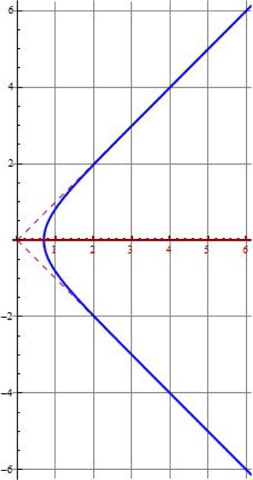
Spacelike curve with 𝓚(y) = sinh y.
Acknowledgement
Research of the two first named authors was partially supported by a MEC-FEDER grant MTM2017-89677-P . Research of the third named author was partially supported by a MECD grant FPU16/03096.
References
[1] Singer D., Curves whose curvature depends on distance from the origin, Amer. Math. Monthly, 1999, 106, 835–841.10.1080/00029890.1999.12005128Search in Google Scholar
[2] Singer D., Lectures on elastic curves and rods, Curvature and variational modelling in Physics and Biophysics, AIP Conf. Proc., 2008, 1002, 3–32.10.1063/1.2918095Search in Google Scholar
[3] Djondjorov P.A., Vassilev V-M., Mladenov I.M., Plane curves associated with integrable dynamical systems of the Frenet-Serret type, Proc. of the 9th International Workshop on Complex Structures, Integrability and Vector Fields, World Scientific, Singapore, 2009, pp. 57–63.10.1142/9789814277723_0007Search in Google Scholar
[4] Vassilev V.M., Djondjorov P.A., Mladenov I.M., Integrable dynamical systems of the Frenet-Serret type, Proc. of the 9th International Workshop on Complex Structures, Integrability and Vector Fields, World Scientific, Singapore, 2009, pp. 234–244.10.1142/9789814277723_0029Search in Google Scholar
[5] Mladenov I.M., Hadzhilazova M.T., Djondjorov P.A., Vassilev V.M., On the plane curves whose curvature depends on the distance from the origin, XXIX Workshop on Geometric Methods in Physics. AIP Conf. Proc., 2010, 1307, 112–118.10.1063/1.3527406Search in Google Scholar
[6] Mladenov I.M., Hadzhilazova M.T., Djondjorov P.A., Vassilev. V.M., On the generalized Sturmian spirals, C. R. Acad. Sci. Bulg., 2011, 64, 633–640.Search in Google Scholar
[7] Mladenov I.M., Hadzhilazova M.T., Djondjorov P.A., Vassilev V.M., On some deformations of the Cassinian oval, International Workshop on Complex Structures, Integrability and Vector Fields. AIP Conf. Proc., 2011, 1340, 81–89.10.1063/1.3567127Search in Google Scholar
[8] Mladenov I.M., Marinov P.I., Hadzhilazova M.T., Elastic spirals, Workshop on Application of Mathematics in Technical and Natural Sciences. AIP Conf. Proc., 2014, 1629, 437–443.10.1063/1.4902306Search in Google Scholar
[9] Marinov P.I., Hadzhilazova M.T., Mladenov I.M., Elastic Sturmian spirals, C. R. Acad. Sci. Bulg., 2014, 67, 167–172.Search in Google Scholar
[10] Castro I., Castro-Infantes I., Plane curves with curvature depending on distance to a line, Diff. Geom. Appl., 2016, 44, 77–97.10.1016/j.difgeo.2015.11.002Search in Google Scholar
[11] Castro I., Castro-Infantes I., Castro-Infantes, J., New plane curves with curvature depending on distance from the origin, Mediterr. J. Math., 2017, 14, 108:1–19.10.1007/s00009-017-0912-zSearch in Google Scholar
[12] Ilarslan K., Uçum A., Mladenov I.M., Sturmian spirals in Lorentz-Minkowski plane, J. Geom. Symmetry Phys., 2015, 37, 25–42.10.7546/jgsp-37-2015-25-42Search in Google Scholar
[13] Uçum A., Ilarslan K., Mladenov I.M., Elastic Sturmian spirals in Lorentz-Minkowski plane, Open Math., 2016, 14, 1149–1156.10.1515/math-2016-0103Search in Google Scholar
[14] López R., Differential Geometry of Curves and Surfaces in Lorentz-Minkowski sapce, Int. Electron. J. Geom., 2014, 1, 44–107.10.36890/iejg.594497Search in Google Scholar
[15] Saloom A., Tari F., Curves in the Minkowski plane and their contact with pseudo-circles, Geom. Dedicata, 2012, 159, 109–124.10.1007/s10711-011-9649-1Search in Google Scholar
[16] Arroyo J., Garay O.J., Mencía J.J., Closed generalized elastic curves in 𝕊2(1), J. Geom. Phys., 2003, 48, 339–353.10.1016/S0393-0440(03)00047-0Search in Google Scholar
[17] Arroyo J., Garay O.J., Mencía J.J., Elastic curves with constant curvature at rest in the hyperbolic plane, J. Geom. Phys., 2011, 61, 1823–1844.10.1016/j.geomphys.2011.04.006Search in Google Scholar
[18] Bryant R., Griffiths P., Reduction of order for constrained variational problems and ∫γ (κ2/2) ds, Am. J. Math., 1986, 108, 525–570.10.2307/2374654Search in Google Scholar
[19] Jurdjevic V., Non-Euclidean elastica, Amer. J. Math., 1995, 117, 93–124.10.2307/2375037Search in Google Scholar
[20] Langer J., Singer, D., The total squared curvature of closed curves, J. Differential Geom., 1984, 20, 1–22.10.4310/jdg/1214438990Search in Google Scholar
[21] Kobayashi O., Maximal surfaces in the 3-dimensional Minkowski space L3, Tokyo J. Math., 1983, 6, 297–309.10.3836/tjm/1270213872Search in Google Scholar
[22] Angenent S., On the formation of singularities in the curve shortening flow, J. Differential Geom., 1991, 33, 601–633.10.4310/jdg/1214446558Search in Google Scholar
[23] Castro I., Castro-Infantes I., Castro-Infantes J., Curves in Lorentz-Minkowski plane with curvature depending on their position, Preprint arXiv:1806.09187 [math.DG].10.1515/math-2020-0043Search in Google Scholar
[24] Byrd P.F., Friedman M.D., Handbook of elliptic integrals for engineers and physicists, Springer Verlag, 1971.10.1007/978-3-642-65138-0Search in Google Scholar
[25] Sager I., Abazari N., Ekmekci N., Yayli Y., The classical elastic curves in Lorentz-Minkowski space, Int. J. Contemp. Math. Sciences, 2011, 6, 309–320.Search in Google Scholar
© 2018 Castro et al., published by De Gruyter
This work is licensed under the Creative Commons Attribution-NonCommercial-NoDerivatives 4.0 License.
Articles in the same Issue
- Regular Articles
- Algebraic proofs for shallow water bi–Hamiltonian systems for three cocycle of the semi-direct product of Kac–Moody and Virasoro Lie algebras
- On a viscous two-fluid channel flow including evaporation
- Generation of pseudo-random numbers with the use of inverse chaotic transformation
- Singular Cauchy problem for the general Euler-Poisson-Darboux equation
- Ternary and n-ary f-distributive structures
- On the fine Simpson moduli spaces of 1-dimensional sheaves supported on plane quartics
- Evaluation of integrals with hypergeometric and logarithmic functions
- Bounded solutions of self-adjoint second order linear difference equations with periodic coeffients
- Oscillation of first order linear differential equations with several non-monotone delays
- Existence and regularity of mild solutions in some interpolation spaces for functional partial differential equations with nonlocal initial conditions
- The log-concavity of the q-derangement numbers of type B
- Generalized state maps and states on pseudo equality algebras
- Monotone subsequence via ultrapower
- Note on group irregularity strength of disconnected graphs
- On the security of the Courtois-Finiasz-Sendrier signature
- A further study on ordered regular equivalence relations in ordered semihypergroups
- On the structure vector field of a real hypersurface in complex quadric
- Rank relations between a {0, 1}-matrix and its complement
- Lie n superderivations and generalized Lie n superderivations of superalgebras
- Time parallelization scheme with an adaptive time step size for solving stiff initial value problems
- Stability problems and numerical integration on the Lie group SO(3) × R3 × R3
- On some fixed point results for (s, p, α)-contractive mappings in b-metric-like spaces and applications to integral equations
- On algebraic characterization of SSC of the Jahangir’s graph 𝓙n,m
- A greedy algorithm for interval greedoids
- On nonlinear evolution equation of second order in Banach spaces
- A primal-dual approach of weak vector equilibrium problems
- On new strong versions of Browder type theorems
- A Geršgorin-type eigenvalue localization set with n parameters for stochastic matrices
- Restriction conditions on PL(7, 2) codes (3 ≤ |𝓖i| ≤ 7)
- Singular integrals with variable kernel and fractional differentiation in homogeneous Morrey-Herz-type Hardy spaces with variable exponents
- Introduction to disoriented knot theory
- Restricted triangulation on circulant graphs
- Boundedness control sets for linear systems on Lie groups
- Chen’s inequalities for submanifolds in (κ, μ)-contact space form with a semi-symmetric metric connection
- Disjointed sum of products by a novel technique of orthogonalizing ORing
- A parametric linearizing approach for quadratically inequality constrained quadratic programs
- Generalizations of Steffensen’s inequality via the extension of Montgomery identity
- Vector fields satisfying the barycenter property
- On the freeness of hypersurface arrangements consisting of hyperplanes and spheres
- Biderivations of the higher rank Witt algebra without anti-symmetric condition
- Some remarks on spectra of nuclear operators
- Recursive interpolating sequences
- Involutory biquandles and singular knots and links
- Constacyclic codes over 𝔽pm[u1, u2,⋯,uk]/〈 ui2 = ui, uiuj = ujui〉
- Topological entropy for positively weak measure expansive shadowable maps
- Oscillation and non-oscillation of half-linear differential equations with coeffcients determined by functions having mean values
- On 𝓠-regular semigroups
- One kind power mean of the hybrid Gauss sums
- A reduced space branch and bound algorithm for a class of sum of ratios problems
- Some recurrence formulas for the Hermite polynomials and their squares
- A relaxed block splitting preconditioner for complex symmetric indefinite linear systems
- On f - prime radical in ordered semigroups
- Positive solutions of semipositone singular fractional differential systems with a parameter and integral boundary conditions
- Disjoint hypercyclicity equals disjoint supercyclicity for families of Taylor-type operators
- A stochastic differential game of low carbon technology sharing in collaborative innovation system of superior enterprises and inferior enterprises under uncertain environment
- Dynamic behavior analysis of a prey-predator model with ratio-dependent Monod-Haldane functional response
- The points and diameters of quantales
- Directed colimits of some flatness properties and purity of epimorphisms in S-posets
- Super (a, d)-H-antimagic labeling of subdivided graphs
- On the power sum problem of Lucas polynomials and its divisible property
- Existence of solutions for a shear thickening fluid-particle system with non-Newtonian potential
- On generalized P-reducible Finsler manifolds
- On Banach and Kuratowski Theorem, K-Lusin sets and strong sequences
- On the boundedness of square function generated by the Bessel differential operator in weighted Lebesque Lp,α spaces
- On the different kinds of separability of the space of Borel functions
- Curves in the Lorentz-Minkowski plane: elasticae, catenaries and grim-reapers
- Functional analysis method for the M/G/1 queueing model with single working vacation
- Existence of asymptotically periodic solutions for semilinear evolution equations with nonlocal initial conditions
- The existence of solutions to certain type of nonlinear difference-differential equations
- Domination in 4-regular Knödel graphs
- Stepanov-like pseudo almost periodic functions on time scales and applications to dynamic equations with delay
- Algebras of right ample semigroups
- Random attractors for stochastic retarded reaction-diffusion equations with multiplicative white noise on unbounded domains
- Nontrivial periodic solutions to delay difference equations via Morse theory
- A note on the three-way generalization of the Jordan canonical form
- On some varieties of ai-semirings satisfying xp+1 ≈ x
- Abstract-valued Orlicz spaces of range-varying type
- On the recursive properties of one kind hybrid power mean involving two-term exponential sums and Gauss sums
- Arithmetic of generalized Dedekind sums and their modularity
- Multipreconditioned GMRES for simulating stochastic automata networks
- Regularization and error estimates for an inverse heat problem under the conformable derivative
- Transitivity of the εm-relation on (m-idempotent) hyperrings
- Learning Bayesian networks based on bi-velocity discrete particle swarm optimization with mutation operator
- Simultaneous prediction in the generalized linear model
- Two asymptotic expansions for gamma function developed by Windschitl’s formula
- State maps on semihoops
- 𝓜𝓝-convergence and lim-inf𝓜-convergence in partially ordered sets
- Stability and convergence of a local discontinuous Galerkin finite element method for the general Lax equation
- New topology in residuated lattices
- Optimality and duality in set-valued optimization utilizing limit sets
- An improved Schwarz Lemma at the boundary
- Initial layer problem of the Boussinesq system for Rayleigh-Bénard convection with infinite Prandtl number limit
- Toeplitz matrices whose elements are coefficients of Bazilevič functions
- Epi-mild normality
- Nonlinear elastic beam problems with the parameter near resonance
- Orlicz difference bodies
- The Picard group of Brauer-Severi varieties
- Galoisian and qualitative approaches to linear Polyanin-Zaitsev vector fields
- Weak group inverse
- Infinite growth of solutions of second order complex differential equation
- Semi-Hurewicz-Type properties in ditopological texture spaces
- Chaos and bifurcation in the controlled chaotic system
- Translatability and translatable semigroups
- Sharp bounds for partition dimension of generalized Möbius ladders
- Uniqueness theorems for L-functions in the extended Selberg class
- An effective algorithm for globally solving quadratic programs using parametric linearization technique
- Bounds of Strong EMT Strength for certain Subdivision of Star and Bistar
- On categorical aspects of S -quantales
- On the algebraicity of coefficients of half-integral weight mock modular forms
- Dunkl analogue of Szász-mirakjan operators of blending type
- Majorization, “useful” Csiszár divergence and “useful” Zipf-Mandelbrot law
- Global stability of a distributed delayed viral model with general incidence rate
- Analyzing a generalized pest-natural enemy model with nonlinear impulsive control
- Boundary value problems of a discrete generalized beam equation via variational methods
- Common fixed point theorem of six self-mappings in Menger spaces using (CLRST) property
- Periodic and subharmonic solutions for a 2nth-order p-Laplacian difference equation containing both advances and retardations
- Spectrum of free-form Sudoku graphs
- Regularity of fuzzy convergence spaces
- The well-posedness of solution to a compressible non-Newtonian fluid with self-gravitational potential
- On further refinements for Young inequalities
- Pretty good state transfer on 1-sum of star graphs
- On a conjecture about generalized Q-recurrence
- Univariate approximating schemes and their non-tensor product generalization
- Multi-term fractional differential equations with nonlocal boundary conditions
- Homoclinic and heteroclinic solutions to a hepatitis C evolution model
- Regularity of one-sided multilinear fractional maximal functions
- Galois connections between sets of paths and closure operators in simple graphs
- KGSA: A Gravitational Search Algorithm for Multimodal Optimization based on K-Means Niching Technique and a Novel Elitism Strategy
- θ-type Calderón-Zygmund Operators and Commutators in Variable Exponents Herz space
- An integral that counts the zeros of a function
- On rough sets induced by fuzzy relations approach in semigroups
- Computational uncertainty quantification for random non-autonomous second order linear differential equations via adapted gPC: a comparative case study with random Fröbenius method and Monte Carlo simulation
- The fourth order strongly noncanonical operators
- Topical Issue on Cyber-security Mathematics
- Review of Cryptographic Schemes applied to Remote Electronic Voting systems: remaining challenges and the upcoming post-quantum paradigm
- Linearity in decimation-based generators: an improved cryptanalysis on the shrinking generator
- On dynamic network security: A random decentering algorithm on graphs