Stability problems and numerical integration on the Lie group SO(3) × R3 × R3
-


Abstract
The paper is dealing with stability problems for a nonlinear system on the Lie group SO(3) × R3 × R3. The approximate analytic solutions of the considered system via Optimal Homotopy Asymptotic Method are presented, too.
1 Introduction
The optimal control problems on the Lie groups were studied very often in deep connection with mechanical systems. We can find a large list of such examples, like the dynamics of an underwater vehicle, with SE(3, R) = SO(3) × R3 as space configuration (see [1]), the ball-plate problem, with R2 × SO(3) as space configuration [2], the rolling-penny dynamics having the Lie group SE(2, R) × SO(2) as space configuration [3], the control tower problem from air traffic, modeled on the Special Euclidean Group SE(3), the spacecraft dynamics modeled on the special orthogonal group SO(3), [4], the buoyancy’s dynamics on the Lie group SO(3) × R3 × R3, (see [5] for details), and the list may go on.
Similar methods were used in [6,7,8,9,10].
Taking into consideration that in many cases the dynamics can be viewed as a left-invariant, drift-free control system on the considered Lie group, we became interested in the study of such systems. The problem of finding the optimal controls that minimize a quadratic cost function for the general left-invariant drift-free control system
on the Lie group G = SO(3) × R3 × R3, where Ai, i = 1, 9 is the standard basis of the Lie algebra g:
Since the span of the set of Lie brackets generated by A1, A2, A3, A5, A7 coincides with g, the system (1) is controllable [11].
Considering now the cost function given by:
the controls that minimize J and steer the system (1) from X = X0 at t = 0 to X = Xf at t = tf are given by:
where xi’s are solutions of the following nonlinear system:
The main goal of our paper is to establish some stability results of the equilibrium points
of the above system. Some stability results regarding the equilibrium states
were already obtained in [11], but the stability problem for the other equilibrium states remains unsolved.
The paper is organized as follows: in the second paragraph we find an appropriate control function in order to stabilize the equilibrium states
2 Stabilization of
e 6 M N P
Let us employ the control u ∈ C∞ (R9, R),
for the system (2). The controlled system (2)–(3), explicitly given by
has
Proposition 2.1
The controlled system(4)has the Hamilton-Poisson realization
whereG = SO(3) × R3 × R3,
is the minus Lie-Poisson structure on the dual of the corresponding Lie algebrag∗and the Hamiltonian function given by
Proof
Indeed, one obtains immediately that
and Π is a minus Lie-Poisson structure, see for details [11]. □
Remark 2.2
([11]). The functionsC1, C2, C3 : R9 → Rgiven by
and
are the Casimirs of our Poisson configuration.
The goal of this paragraph is to study the spectral and nonlinear stability of the equilibrium state
Let A be the matrix of linear part of our controlled system (4), that is
At the equilibrium of interest its characteristic polynomial has the following expression:
Hence we have five zero eigenvalues and four purely imaginary eigenvalues. So we can conclude:
Proposition 2.3
The controlled system(4)may be spectral stabilized about the equilibrium states
Moreover we can prove:
Proposition 2.4
The controlled system(4)may be nonlinear stabilized about the equilibrium states
Proof
For the proof we shall use Arnold’s technique. Let us consider the following function
The following conditions hold:
Considering now
then, for all v ∈ W, i.e. v = (a, b, c, 0, d, e,0, f, g), a, b, c, d, e, f, g ∈ R we have
which is positive definite under the restriction λ > 0, and so
is positive definite.
Therefore, via Arnold’s technique, the equilibrium states
3 Basic ideas of the Optimal Homotopy Asymptotic Method
In order to compute analytical approximate solutions for the nonlinear differential system given by the equations (4) with the boundary conditions
we will use the Optimal Homotopy Asymptotic Method (OHAM) [12,13,14].
Let us start with a very short description of this method. The analytical approximate solutions can be obtained for equations of the general form:
subject to the initial conditions of the type:
where L is a linear operator (which is not unique), N is a nonlinear one and x(t) is the unknown smooth function of the Eq. (7).
Following [12,13,14], we construct the homotopy given by:
where p ∈ [0, 1] is the embedding parameter, H(t, Ci ), (H ≠ 0) is an auxiliary convergence-control function, depending on the variable t and on the parameters C1, C2, …, Cs and the function x(t, p) has the expression:
The following properties hold:
and
The governing equations of X0(t) and x1(t, Ci) can be obtained by equating the coefficients of p0 and p1, respectively:
The expression of x0(t) can be found by solving the linear equation (13). Also, to compute x1(t, Ci) we solve the equation (14), by taking into consideration that the nonlinear operator N presents the general form:
where m is a positive integer and hi(t) and gi(t) are known functions depending both on x0(t) and N.
Although the equation (14) is a nonhomogeneous linear one, in the most cases its solution can not be found.
In order to compute the function x1(t, Ci) we will use the third modified version of OHAM (see [14] for details), consisting in the following steps:
First we consider one of the following expressions for x1(t, Ci):
or
These expressions of Hi(t, hj(t), Cj) contain both linear combinations of the functions hj and the parameters Cj, j = 1, s. The summation limit m is an arbitrary positive integer number.
Next, by taking into account the equation (10), for p = 1, the first-order analytical approximate solution of the equations (7) - (8) is:
Finally, the convergence-control parameters C1, C2, …, Cs, which determine the first-order approximate solution (18), can be optimally computed by means of various methods, such as: the least square method, the Galerkin method, the collocation method, the Kantorowich method or the weighted residual method.
Definition 3.1
[15] We call anε-approximate solutionof the problem (7) on the domain (0, ∞) a smooth functionx(t, Ci) of the form (18) which satisfies the following condition:
together with the initial condition from Eq. (8), where the residual functionR(t, x(t, Ci)) is obtained by substituting the Eq. (18) into Eq. (7), i.e.
4 Application of Optimal Homotopy Asymptotic Method for solving the nonlinear differential system (4)
In order to solve the nonlinear differential system given by the equations (4), each equation of the system (4) can be written in the form Eq. (7), where we can choose the linear operators as:
with K > 0, K1 > 0 the unknown parameters at this moment.
The corresponding linear equations for initial approximations xi0, i = 1, 9 can be obtained by means of the Eqs. (13), (19) and (6):
whose solutions are
The corresponding nonlinear operators N[xi(t)], i = 1, 9 are obtained from the equations (4):
such that
and therefore, substituting Eqs. (21) into Eqs. (22), we obtain
Remark 4.1
Now, we observe that the nonlinear operators N[xi0(t)], i = 1, 9are the linear combinations between the elementary functionse–K1t · cos(Mt), e–K1t · sin(Mt), e–2K1t · cos2(Mt), e–2K1t · sin2(Mt), e–2K1t · cos(Mt) sin(Mt), e–K1t · cos(Kt), e–K1t · sin(Kt), e–2K1t · cos(Kt) cos(Mt), e–2K1t · sin(Kt) sin(Mt), e–2K1t · cos(Kt) sin(Mt), e–2K1t · sin(Kt) cos(Mt).
On the other hand, the Eq. (14) becomes:
where the linear operators L are given by Eq. (19) and the expressions N(xi0(t)), i = 1, 9 are given by Eq. (23).
The auxiliary convergence-control functions Hi are chosen such that the product between hi · N[xi0(t)] has the same form of the N[xi0(t)]. Then, the first approximation becomes:
Using now the third-alternative of OHAM and the equations (18), the first-order approximate solution can be put in the form
where xi0(t) and xi1(t, Ci) are given by (21) and (25), respectively.
5 Numerical examples and discussions
In this section, the accuracy and validity of the OHAM technique is proved using a comparison of our approximate solutions with numerical results obtained via the fourth-order Runge-Kutta method in the following case: we consider the initial value problem given by (4) with initial conditions (6)Ai = 0.0001, i = 1, 9, M = 15 and P = 20.
One can show that these approximate solutions are weekε-approximate solutions by computing the numerical value of the integral of square residual function (to see the Table 4),
The comparison between the approximate solutions x̄3 given by Eq. (30) and the corresponding numerical solutions for M = 15 and P = 20 (relative errors: εx3 = |x3numerical – x̄3OHAM|)
| t | X3numerical | x3oham given by Eq.(30) | εx3 |
|---|---|---|---|
| 0 | 0.0001 | 0.0001 | 0 |
| 1/10 | –0.00026388686019 | –0.00026388920732 | 2.34712908 ·10–9 |
| 1/5 | –0.00098972163690 | –0.00098972743135 | 5.79444527 ·10–9 |
| 3/10 | 0.00080121591193 | 0.00080121516755 | 7.44372891 ·10–10 |
| 2/5 | 0.00205113177145 | 0.00205113953903 | 7.76758435 ·10–9 |
| 1/2 | –0.00105407568168 | –0.00105407578483 | 1.03151043 ·10–10 |
| 3/5 | –0.00322482848832 | –0.00322483170127 | 3.21294763 ·10–9 |
| 7/10 | 0.00099573781977 | 0.00099573897878 | 1.15901067 ·10–9 |
| 4/5 | 0.00444604275839 | 0.00444604908979 | 6.33140294 ·10–9 |
| 9/10 | –0.00061159885752 | –0.00061159746243 | 1.39509107 ·10–9 |
| 1 | –0.00564686848672 | –0.00564687685941 | 8.37269479 ·10–9 |
The comparison between the approximate solutions x̄5 given by Eq. (32) and the corresponding numerical solutions for M = 15 and P = 20 (relative errors: εx5 = |x5numerical – x̄5OHAM|)
| t | X5numerical | x5oham given by Eq.(32) | εx5 |
|---|---|---|---|
| 0 | 0 0.0001 | 0.0001 | 0 |
| 1/10 | –0.00009267394569 | –0.00009267384041 | 1.05273724 ·10–10 |
| 1/5 | –0.00011309924594 | –0.00011309966129 | 4.15348823 ·10–10 |
| 3/10 | 0.00007665834993 | 0.00007665851028 | 1.60350492 ·10–10 |
| 2/5 | 0.00012391598733 | 0.00012391636093 | 3.73592167 ·10–10 |
| 1/2 | –0.00005910519311 | –0.00005910537099 | 1.77875786 ·10–10 |
| 3/5 | –0.00013222655382 | –0.00013222667316 | 1.19336773 ·10–10 |
| 7/10 | 0.00004037430382 | 0.00004037416907 | 1.34745601 ·10–10 |
| 4/5 | 0.00013786222359 | 0.00013786239690 | 1.73302447 ·10–10 |
| 9/10 | –0.00002084981273 | –0.00002084984022 | 2.74919318 ·10–11 |
| 1 | –0.00014071144636 | –0.00014071122544 | 2.20921854 ·10–10 |
The comparison between the approximate solutions x̄8 given by Eq. (35) and the corresponding numerical solutions for M = 15 and P = 20 (relative errors: εx8 = |x8numerical – x̄8OHAM|)
| t | X8numerical | x8oham given by Eq.(32) | εx8 |
|---|---|---|---|
| 0 | 0.0001 | 0.0001 | 0 |
| 1/10 | –0.00009267394569 | –0.00009267384041 | 1.05273724 ·10–10 |
| 1/5 | –0.00011309924594 | –0.00011309966129 | 4.15348823 ·10–10 |
| 3/10 | 0.00007665834993 | 0.00007665851028 | 1.60350492 ·10–10 |
| 2/5 | 0.00012391598733 | 0.00012391636093 | 3.73592167 ·10–10 |
| 1/2 | –0.00005910519311 | –0.00005910537099 | 1.77875786 ·10–10 |
| 3/5 | –0.00013222655382 | –0.00013222667316 | 1.19336773 ·10–10 |
| 7/10 | 0.00004037430382 | 0.00004037416907 | 1.34745601 ·10–10 |
| 4/5 | 0.00013786222359 | 0.00013786239690 | 1.73302447 ·10–10 |
| 9/10 | –0.00002084981273 | –0.00002084984022 | 2.74919318 ·10–11 |
| 1 | –0.00014071144636 | –0.00014071122544 | 2.20921854 ·10–10 |
The numerical values of the integral of square residual function given by Eq. (27) corresponding to the approximate solutions given by Eqs. (28)-(36) for M = 15 and P = 20
| i | |
|---|---|
| 1 | 7.464737808519274 ·10–17 |
| 2 | 8.459118984995915 ·10–13 |
| 3 | 1.0225368942228159 ·10–13 |
| 4 | 2.6769875640036004 ·10–23 |
| 5 | 9.659432242298964 ·10–17 |
| 6 | 8.086505295586057 ·10–17 |
| 7 | 1.4525406989853368 ·10–23 |
| 8 | 9.659432355712418 ·10–17 |
| 9 | 8.086505295410683 ·10–17 |
where
with x̄i(t), i = 1, …, 9 given by Eq. (26).
The convergence-control parameters K, K1, ω, Bi, Ci, i = 1, 9 are optimally determined by means of the least-square method.
for x̄1 : The convergence-control parameters are respectively:
The first-order approximate solutions given by the Eq. (26) are respectively:
For all unknown functions x̄i, i = 1, 9, we have K1 = 0.58656793719790 and ω = 1.01132823106464.
for x̄2:
for x̄3:
for x̄4:
for x̄5:
for x̄6:
for x̄7:
for x̄8:
for x̄9:
Finally, Tables 1, 2 and 3 emphasizes the accuracy of the OHAM technique by comparing the approximate analytic solutions x̄3, x̄5 and x̄8 respectively presented above with the corresponding numerical integration values.
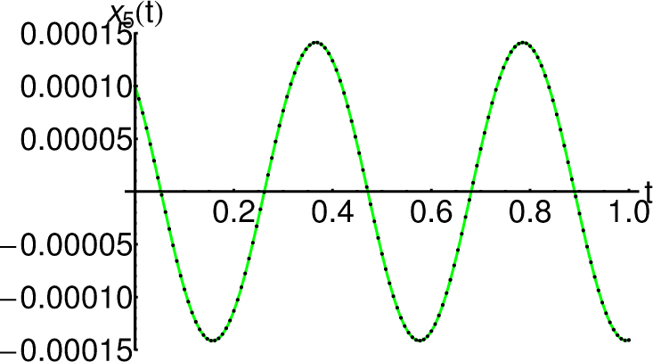
The Figs. 1-9 depicted a comparison between the obtained approximate solutions given by Eqs. (28)-(36) with corresponding numerical integration.

Comparison between the approximate solutions x̄1 given by Eq. (28) and the corresponding numerical solutions
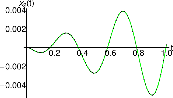
Comparison between the approximate solutions x̄2 given by Eq. (29) and the corresponding numerical solutions
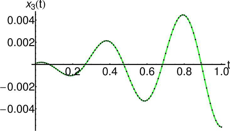
Comparison between the approximate solutions x̄3 given by Eq. (30) and the corresponding numerical solutions
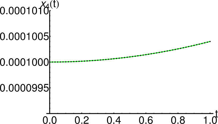
Comparison between the approximate solutions x̄4 given by Eq. (31) and the corresponding numerical solutions

Comparison between the approximate solutions x̄5 given by Eq. (32) and the corresponding numerical solutions
Comparison between the approximate solutions x̄6 given by Eq. (33) and the corresponding numerical solutions
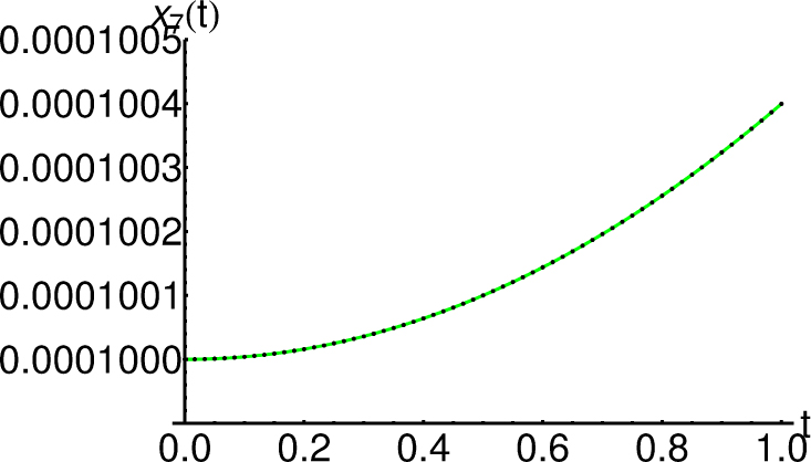
Comparison between the approximate solutions x̄7 given by Eq. (34) and the corresponding numerical solutions
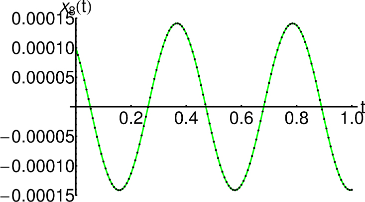
Comparison between the approximate solutions x̄8 given by Eq. (35) and the corresponding numerical solutions
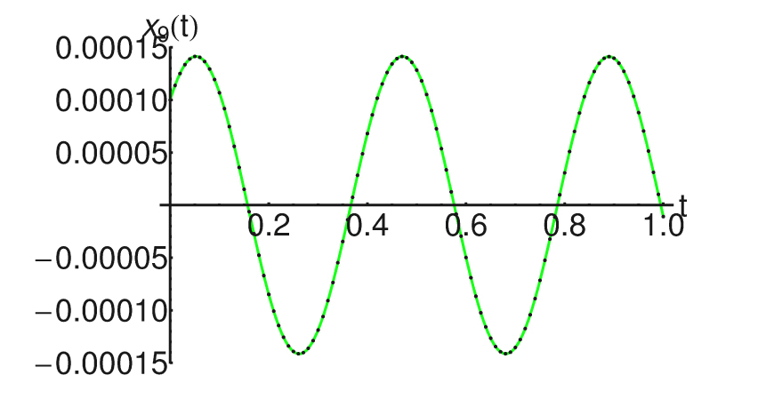
Comparison between the approximate solutions x̄9 given by Eq. (36) and the corresponding numerical solutions
6 Conclusion
The paper presents the stabilization of a dynamical system using a linear control function. The Hamilton-Poisson formulation of the obtained system allows to use energy-methods in order to obtain stability results. In the last section the approximate analytic solutions of the considered controlled system (4) are established using the optimal homotopy asymptotic method (OHAM). Numerical simulations via Mathematica 9.0 software and the approximations deviations are presented. The accuracy of our results is pointed out by means of the approximate residual of the solutions.
The next step we intend to do is a comparison between the Lie-Trotter integrator (which is a Poisson one, see [11]) and OHAM, regarding the numerical results.
Conflict of interest
Conflict of interests: The authors declare that there is no conflict of interests regarding the publication of this paper.
References
[1] Birtea P., Puta M., and Tudoran R., Some remarks on the dynamics of the underwater vehicle, Bull. Sci. Math., 2007, 131(7), 601–612.10.1016/j.bulsci.2006.04.001Search in Google Scholar
[2] Jurdjevic V., The geometry of the ball-plate problem, Arch. Rat. Mech. Anal., 1993, 124, 305–328.10.1007/BF00375605Search in Google Scholar
[3] Aron A., Pop C., and Puta M., An optimal control problem on the Lie group SE(2, R) × SO(2), Bol. Soc. Mat. Mex. (3), 2009, 15, 13 pages.Search in Google Scholar
[4] Leonard N. E., Averaging and motion control systems on Lie groups, Ph.D. Thesis, University of Maryland, College Park, MD, 1994.Search in Google Scholar
[5] Narayanan V., Morrison P. J., Rank change in Poisson dynamical systems, http://arxiv.org/abs/1302.7267.Search in Google Scholar
[6] Bloch A. M., Krishnaprasad P. S., Marsden J. E., Sanchez de Alvarez G., Stabilization of Rigid Body Dynamics by Internal and External Torques, Automatica, 1992, 28, 745–756.10.1016/0005-1098(92)90034-DSearch in Google Scholar
[7] Pop C., Aron A., Petrişor C., Geometrical Aspects of the Ball-Plate Problem, Balk. J. Geom. Appl., 2011, 16(2), 114–122.Search in Google Scholar
[8] Pop Arieşanu C., Stability Problems for Chua System with One Linear Control, Journal of Applied Mathematics, 2013, Article ID 764108, http://dx.doi.org/10.1155/2013/764108.10.1155/2013/764108Search in Google Scholar
[9] Puta M., On the Maxwell-Bloch equations with one control, C. R. Acad. Sci. Paris, Serie 1, 1994, 318, 679–683.Search in Google Scholar
[10] Puta M., On an Extension of the 3-Dimensional Toda Lattice, Preprint ESI, Vienna, 1996, 165, http://www.esi.ac.atstatic/esiprpr/esi165.pdfSearch in Google Scholar
[11] Pop C., Free Left Invariant Control System on the Lie Group SO(3) × R3 × R3, Math. Probl. Eng., 2015, Article ID 652819,10.1155/2015/652819.Search in Google Scholar
[12] Marinca V., Herişanu N., Nonlinear dynamic analysis of an electrical machine rotor-bearing system by the optimal homotopy perturbation method, Comput. Math. Appl., 2011, 61, 2019–2024.10.1016/j.camwa.2010.08.056Search in Google Scholar
[13] Marinca V., Herişanu N., Bota C., Marinca B., An optimal homotopy asymptotic method applied to the steady flow of a fourth grade fluid past a porous plate, Appl. Math. Lett., 2009, 22, 245–251.10.1016/j.aml.2008.03.019Search in Google Scholar
[14] Marinca V., Herişanu N., The Optimal Homotopy Asymptotic Method: Engineering Applications, Springer Verlag, Heidelberg, 2015.10.1007/978-3-319-15374-2Search in Google Scholar
[15] Bota C., Căruntu B., Approximate analytical solutions of the regularized long wave equation using the optimal homotopy perturbation method, Sci. World. J., 2014, Article ID: 721865, 6 pages.10.1155/2014/721865Search in Google Scholar PubMed PubMed Central
© 2018 Pop and Ene, published by De Gruyter
This work is licensed under the Creative Commons Attribution-NonCommercial-NoDerivatives 4.0 License.
Articles in the same Issue
- Regular Articles
- Algebraic proofs for shallow water bi–Hamiltonian systems for three cocycle of the semi-direct product of Kac–Moody and Virasoro Lie algebras
- On a viscous two-fluid channel flow including evaporation
- Generation of pseudo-random numbers with the use of inverse chaotic transformation
- Singular Cauchy problem for the general Euler-Poisson-Darboux equation
- Ternary and n-ary f-distributive structures
- On the fine Simpson moduli spaces of 1-dimensional sheaves supported on plane quartics
- Evaluation of integrals with hypergeometric and logarithmic functions
- Bounded solutions of self-adjoint second order linear difference equations with periodic coeffients
- Oscillation of first order linear differential equations with several non-monotone delays
- Existence and regularity of mild solutions in some interpolation spaces for functional partial differential equations with nonlocal initial conditions
- The log-concavity of the q-derangement numbers of type B
- Generalized state maps and states on pseudo equality algebras
- Monotone subsequence via ultrapower
- Note on group irregularity strength of disconnected graphs
- On the security of the Courtois-Finiasz-Sendrier signature
- A further study on ordered regular equivalence relations in ordered semihypergroups
- On the structure vector field of a real hypersurface in complex quadric
- Rank relations between a {0, 1}-matrix and its complement
- Lie n superderivations and generalized Lie n superderivations of superalgebras
- Time parallelization scheme with an adaptive time step size for solving stiff initial value problems
- Stability problems and numerical integration on the Lie group SO(3) × R3 × R3
- On some fixed point results for (s, p, α)-contractive mappings in b-metric-like spaces and applications to integral equations
- On algebraic characterization of SSC of the Jahangir’s graph 𝓙n,m
- A greedy algorithm for interval greedoids
- On nonlinear evolution equation of second order in Banach spaces
- A primal-dual approach of weak vector equilibrium problems
- On new strong versions of Browder type theorems
- A Geršgorin-type eigenvalue localization set with n parameters for stochastic matrices
- Restriction conditions on PL(7, 2) codes (3 ≤ |𝓖i| ≤ 7)
- Singular integrals with variable kernel and fractional differentiation in homogeneous Morrey-Herz-type Hardy spaces with variable exponents
- Introduction to disoriented knot theory
- Restricted triangulation on circulant graphs
- Boundedness control sets for linear systems on Lie groups
- Chen’s inequalities for submanifolds in (κ, μ)-contact space form with a semi-symmetric metric connection
- Disjointed sum of products by a novel technique of orthogonalizing ORing
- A parametric linearizing approach for quadratically inequality constrained quadratic programs
- Generalizations of Steffensen’s inequality via the extension of Montgomery identity
- Vector fields satisfying the barycenter property
- On the freeness of hypersurface arrangements consisting of hyperplanes and spheres
- Biderivations of the higher rank Witt algebra without anti-symmetric condition
- Some remarks on spectra of nuclear operators
- Recursive interpolating sequences
- Involutory biquandles and singular knots and links
- Constacyclic codes over 𝔽pm[u1, u2,⋯,uk]/〈 ui2 = ui, uiuj = ujui〉
- Topological entropy for positively weak measure expansive shadowable maps
- Oscillation and non-oscillation of half-linear differential equations with coeffcients determined by functions having mean values
- On 𝓠-regular semigroups
- One kind power mean of the hybrid Gauss sums
- A reduced space branch and bound algorithm for a class of sum of ratios problems
- Some recurrence formulas for the Hermite polynomials and their squares
- A relaxed block splitting preconditioner for complex symmetric indefinite linear systems
- On f - prime radical in ordered semigroups
- Positive solutions of semipositone singular fractional differential systems with a parameter and integral boundary conditions
- Disjoint hypercyclicity equals disjoint supercyclicity for families of Taylor-type operators
- A stochastic differential game of low carbon technology sharing in collaborative innovation system of superior enterprises and inferior enterprises under uncertain environment
- Dynamic behavior analysis of a prey-predator model with ratio-dependent Monod-Haldane functional response
- The points and diameters of quantales
- Directed colimits of some flatness properties and purity of epimorphisms in S-posets
- Super (a, d)-H-antimagic labeling of subdivided graphs
- On the power sum problem of Lucas polynomials and its divisible property
- Existence of solutions for a shear thickening fluid-particle system with non-Newtonian potential
- On generalized P-reducible Finsler manifolds
- On Banach and Kuratowski Theorem, K-Lusin sets and strong sequences
- On the boundedness of square function generated by the Bessel differential operator in weighted Lebesque Lp,α spaces
- On the different kinds of separability of the space of Borel functions
- Curves in the Lorentz-Minkowski plane: elasticae, catenaries and grim-reapers
- Functional analysis method for the M/G/1 queueing model with single working vacation
- Existence of asymptotically periodic solutions for semilinear evolution equations with nonlocal initial conditions
- The existence of solutions to certain type of nonlinear difference-differential equations
- Domination in 4-regular Knödel graphs
- Stepanov-like pseudo almost periodic functions on time scales and applications to dynamic equations with delay
- Algebras of right ample semigroups
- Random attractors for stochastic retarded reaction-diffusion equations with multiplicative white noise on unbounded domains
- Nontrivial periodic solutions to delay difference equations via Morse theory
- A note on the three-way generalization of the Jordan canonical form
- On some varieties of ai-semirings satisfying xp+1 ≈ x
- Abstract-valued Orlicz spaces of range-varying type
- On the recursive properties of one kind hybrid power mean involving two-term exponential sums and Gauss sums
- Arithmetic of generalized Dedekind sums and their modularity
- Multipreconditioned GMRES for simulating stochastic automata networks
- Regularization and error estimates for an inverse heat problem under the conformable derivative
- Transitivity of the εm-relation on (m-idempotent) hyperrings
- Learning Bayesian networks based on bi-velocity discrete particle swarm optimization with mutation operator
- Simultaneous prediction in the generalized linear model
- Two asymptotic expansions for gamma function developed by Windschitl’s formula
- State maps on semihoops
- 𝓜𝓝-convergence and lim-inf𝓜-convergence in partially ordered sets
- Stability and convergence of a local discontinuous Galerkin finite element method for the general Lax equation
- New topology in residuated lattices
- Optimality and duality in set-valued optimization utilizing limit sets
- An improved Schwarz Lemma at the boundary
- Initial layer problem of the Boussinesq system for Rayleigh-Bénard convection with infinite Prandtl number limit
- Toeplitz matrices whose elements are coefficients of Bazilevič functions
- Epi-mild normality
- Nonlinear elastic beam problems with the parameter near resonance
- Orlicz difference bodies
- The Picard group of Brauer-Severi varieties
- Galoisian and qualitative approaches to linear Polyanin-Zaitsev vector fields
- Weak group inverse
- Infinite growth of solutions of second order complex differential equation
- Semi-Hurewicz-Type properties in ditopological texture spaces
- Chaos and bifurcation in the controlled chaotic system
- Translatability and translatable semigroups
- Sharp bounds for partition dimension of generalized Möbius ladders
- Uniqueness theorems for L-functions in the extended Selberg class
- An effective algorithm for globally solving quadratic programs using parametric linearization technique
- Bounds of Strong EMT Strength for certain Subdivision of Star and Bistar
- On categorical aspects of S -quantales
- On the algebraicity of coefficients of half-integral weight mock modular forms
- Dunkl analogue of Szász-mirakjan operators of blending type
- Majorization, “useful” Csiszár divergence and “useful” Zipf-Mandelbrot law
- Global stability of a distributed delayed viral model with general incidence rate
- Analyzing a generalized pest-natural enemy model with nonlinear impulsive control
- Boundary value problems of a discrete generalized beam equation via variational methods
- Common fixed point theorem of six self-mappings in Menger spaces using (CLRST) property
- Periodic and subharmonic solutions for a 2nth-order p-Laplacian difference equation containing both advances and retardations
- Spectrum of free-form Sudoku graphs
- Regularity of fuzzy convergence spaces
- The well-posedness of solution to a compressible non-Newtonian fluid with self-gravitational potential
- On further refinements for Young inequalities
- Pretty good state transfer on 1-sum of star graphs
- On a conjecture about generalized Q-recurrence
- Univariate approximating schemes and their non-tensor product generalization
- Multi-term fractional differential equations with nonlocal boundary conditions
- Homoclinic and heteroclinic solutions to a hepatitis C evolution model
- Regularity of one-sided multilinear fractional maximal functions
- Galois connections between sets of paths and closure operators in simple graphs
- KGSA: A Gravitational Search Algorithm for Multimodal Optimization based on K-Means Niching Technique and a Novel Elitism Strategy
- θ-type Calderón-Zygmund Operators and Commutators in Variable Exponents Herz space
- An integral that counts the zeros of a function
- On rough sets induced by fuzzy relations approach in semigroups
- Computational uncertainty quantification for random non-autonomous second order linear differential equations via adapted gPC: a comparative case study with random Fröbenius method and Monte Carlo simulation
- The fourth order strongly noncanonical operators
- Topical Issue on Cyber-security Mathematics
- Review of Cryptographic Schemes applied to Remote Electronic Voting systems: remaining challenges and the upcoming post-quantum paradigm
- Linearity in decimation-based generators: an improved cryptanalysis on the shrinking generator
- On dynamic network security: A random decentering algorithm on graphs