Flash flood susceptibility mapping using LiDAR-Derived DEM and machine learning algorithms: Ljuboviđa case study, Serbia
-
Siniša Drobnjak

 ,
Zlatan Milonjić
,
Dejan Đorđević
and
Marko Simić
,
Zlatan Milonjić
,
Dejan Đorđević
and
Marko Simić

Abstract
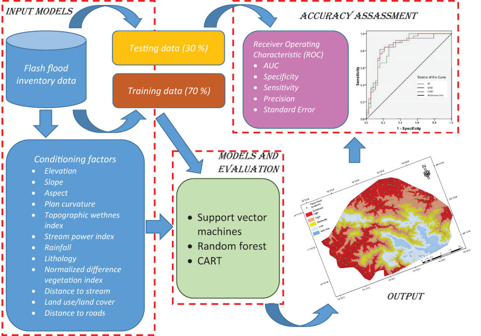
Flash floods are the result of climatic and hydrological extremes and are manifested by dynamic and complex processes of movement of water and sediment. They represent the most frequent and widespread natural disaster at the global level, with unwanted ecological and economic consequences. The main causes of flash floods are related to numerous meteorological and physical–geographical factors. In the territory of Serbia, flash floods represent the most common natural risk with serious consequences for people’s lives and activities. Flash flood susceptibility mapping plays a crucial role in flood risk assessment and management. The current study prepared a flood inventory using light detection and ranging (LiDAR) derived digital elevation model, and it used integrated tree machine learning models (random forest [RF], classification and regression trees [CART], and support vector machine [SVM]) to predict flood susceptibility in the Ljuboviđa watershed, municipality Ljubovija, western Serbia. First, 12 independent variables were employed as conditioning factors: lithology, rainfall, land use/cover, elevation, slope angle, aspect, plan curvature, topographic wetness index, stream power index, distance from streams, distance from roads, and normalized vegetation index. Using the well-known scikit-learn (train_test_split) Python module, the flood inventory dataset was split into 70 and 30% for training and validation, respectively. The models’ performance was additionally assessed using the area under the curve (AUC). The results of the accuracy assessment demonstrated that the models for predicting flood susceptibility, RF, CART, and SVM, had AUC values of 0.854, 0.802, and 0.831, respectively; it means that RF had 85.4%, CART 80.2%, and SVM 83.1% chance of correctly ranking a random positive example higher than a random negative example, which represents the predictive power of the used models. When it came to predicting flood susceptibility, the RF model outperformed the other models used. This model estimates that 15.49, 16.04, 15.67, 23.10, and 29.70% of the watershed are very low, low, moderate, high, and extremely highly susceptible to floods, respectively. Thus, our study shows that data produced from LiDAR is potentially helpful in managing flood risk, particularly when assessing flood-related issues in the future. Flash-flood susceptibility maps have become a vital tool for risk prevention and management for government and local authorities (particularly national and local civil protection agencies, urban planning and land management departments, Ministries of Water and Environment), emergency response services (police, fire, and medical services), infrastructure and utilities sectors, insurance companies, and others.
Graphical abstract
1 Introduction
Throughout history, people have most often built their settlements next to rivers. In addition to satisfying their own needs for drinking and maintaining personal hygiene, rivers were a source of food for them, indirectly, by irrigating agricultural areas, or directly, by fishing. The biggest problem was the occurrence of flood waves. Since the houses of that time were not made of solid material, based on the experience gained, settlements were built outside the inundation zone, outside the river beds and banks that were flooded [1,2]. Therefore, in the history of mankind, floods represent one of the most frequent natural disasters at the global, regional, and local level, causing great damage in urbanized and rural areas, infrastructure, and natural ecosystems [3]. Flooding is a real and constant threat to human communities, infrastructure facilities, and environmental quality around the world [4,5,6,7]. Climate change increases the intensity and frequency of extreme climatic and meteorological events, which affects the frequency and intensity of floods. In the period from 2010 to 2025, floods in 74 countries claimed over 110,000 human lives and caused property damage estimated at more than 1,371 billion dollars [8,9].
Despite great efforts to reduce the risk and mitigate the consequences of floods, as well as through investing large sums of money to defend against these natural disasters, they still cause great material damage and a significant number of human casualties. The probabilistic trends of extreme floods, which are based on climate projections and socio-economic development, indicate an increase in extreme precipitation, as well as the fact that in the coming decades, twice as many flood events can be expected, with a return period of more than 100 years [10,11].
Flash floods belong to a group of natural hydrological disasters characterized by the sudden appearance of maximum flows, with a high concentration of solid phase. Flash floods are localized hydrological phenomena associated with watersheds with pronounced slopes, relatively small areas (from a few km2 to several hundred km2), with a quick reaction to heavy downpours lasting up to several hours [12].
Flash floods are the result of climatic and hydrological extremes and are manifested by dynamic and complex processes of movement of water and sediment. They represent the most frequent and widespread natural disaster at the global level, with undesirable ecological and economic consequences. The main causes of flash floods are related to numerous meteorological and physical–geographical factors. In the territory of Serbia, flash floods represent the most common natural risk with serious consequences for people’s lives and activities [13,14].
Machine learning algorithms are currently utilized to analyze flash flood susceptibility in various regions by combining them with remote sensing data and GIS [5,15,16,17,18]. These artificial intelligence models used for flood mapping are numerous and varied, progressing from simple algorithms to complex hybrid systems [4,6,19]. Further examination of these techniques reveals that linear and kernel-based machine learning algorithms, in particular support vector machines (SVMs), are effective when dimensionality exceeds the amount of data, as demonstrated by models like SVM. However, the effectiveness of this model is often influenced by its kernel values and regularization options [20,21].
Tools like classification and regression trees (CART), which fall within the tree and rule-based models category, exhibit promise as transparent entities that can assess a range of data and skillfully explain nonlinear linkages, despite their susceptibility to issues like overfitting.
To predict flash floods, ensemble and meta-learners that combine many algorithms have demonstrated promise in capturing complex nonlinear interactions in hydrological data [22,23]. Conglomerate models, like random forest (RF), combine several models to provide the best possible prediction performance [11,24]. To increase the randomness of tree growth, RF algorithms look for the best feature from a random selection of features rather than the best feature when splitting a node. As a result, the tree variety increases, producing a stronger model overall.
This article’s primary objective was to develop machine learning models for flash flood susceptibility prediction, compare and evaluate the prediction performance of the aforementioned machine learning models in the western Serbian Ljuboviđa river basin. For the machine learning model, we retrieved 12 factors, including topography and geomorphological factors, hydrological factors, land cover factors, and human activities, using light detection and ranging (LiDAR)-derived digital elevation model (DEM), remotely sensed imagery, meteorological, geological, and topographic data. The susceptibility to flash floods was then analyzed using the SVM, CART, and RF models. Lastly, using the receiver operating characteristic (ROC) curve and susceptibility index distribution features, the prediction performance of each model is compared and examined to confirm its applicability and dependability. One of the main research objectives in this work was determining the extent to which LiDAR-based digital terrain model (DTM) improves the results of flash-flood susceptibility mapping. The results demonstrated that the LiDAR-based DTM improved drainage delineation, increasing the accuracy of flood susceptibility mapping. The results show that the LiDAR-based DTM fared better than the other DTMs in mapping susceptibility and characterizing local drainage patterns.
2 Materials and methods
2.1 Study area
The study area covers approximately 537.55 km2 between the latitudes 44°08′ to 44°21′N and the longitudes 19°20′ to 19°45′E and is located in the western part of the Republic of Serbia (Figure 1). The study area includes parts of Kolubara District and Mačva District. The elevation of the study area ranges from 162 to 1250 m a.m.s.l, with an average altitude of 584.3 m, and with a standard deviation of 219.7 m. There are plains (Kašica, Donja i Gornja Ljuboviđa, Gračanica) and mountains (Bobija, Medvednik, Ranjenica, Nemić) in the study area, making it diverse in terms of the complexity of the topography.
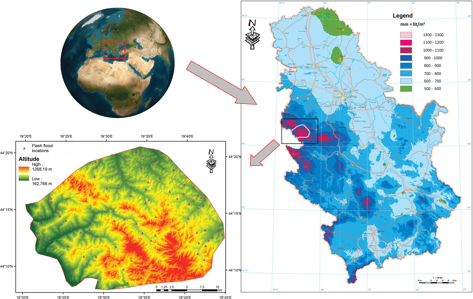
Location of the study area (parts of Kolubara and Mačva District).
In the past, the test area has experienced larger, more intense flash floods. The largest ones occurred on November 18, 1979, May 30, 1985, June 21, 2001, May 14, 2014, and June 22, 2020 [25]. The total annual rainfall in the different parts of the study region ranges from 913.34 to 1205.33 mm. According to records obtained from the Serbian Meteorological Service [26], the maximum rainfall occurs between March and June.
2.2 Data used
A crucial stage in the mapping of flash flood susceptibility is the creation of the inventory map. A flash flood inventory map shows one or more instances of previous floods in a particular location. For flood susceptibility mapping, it is crucial to have an inventory map that shows past flash flood occurrences. Making accurate predictions about future flash flood events in a location requires evaluating the historical records of flash floods. In this study, we used aerial images, field surveys, and high-resolution WorldView 2 imagery to map the flooded area. The study’s flash flood inventory data, which includes 105 recorded flash floods, spans the years 2012–2024.
A further important subject that has been studied by numerous scientists is the flash flood conditioning factors. In order to assess the risk of flash floods, this study used a number of factors, including elevation, slope, aspect, plan curvature, topographic wetness index (TWI), stream power index (SPI), normalized difference vegetation index (NDVI), rainfall, land cover/use (LULC), lithology, and the distance to the stream and roads. Details about the origins of the flash flood conditioning factors are provided in Table 1.
Data used in the susceptibility assessment, the data sources, and the associated factor classes for the flash flood susceptibility mapping in the study area
| Sub-classification | Data Layers | Source of data | Data type | Derived map | Scale or resolution |
|---|---|---|---|---|---|
| Flash flood inventory database | Historic flash floods | Field survey, high-resolution images, and aerial photo interpretation methods | Polygon | — | — |
| Elevation | DEM generated by LiDAR Leica ALS80 only ground data | Grid | Elevation | 1 m | |
| Slope | DEM generated by LiDAR Leica ALS80 only ground data | Grid | Slope gradient (in degrees) | 1 m | |
| Aspect | DEM generated by LiDAR Leica ALS80 only ground data | Grid | Aspect | 1 m | |
| Curvaure | DEM generated by LiDAR Leica ALS80 only ground data | Grid | Plan curvature | 1 m | |
| TWI | DEM generated by LiDAR Leica ALS80 only ground data | Grid | TWI | 1 m | |
| SPI | DEM generated by LiDAR Leica ALS80 only ground data | Grid | SPI | 1 m | |
| Geology map | Litho types | Ministry of Energy, Development and Environmental Protection of the Republic of Serbia http://geoliss.mre.gov.rs/?lang=en | Arc/Info coverage | Lithology | 1:100,000 |
| Land use type | Land use | CORINE 2018 data set – vector https://doi.org/10.2909/71c95a07-e296-44fc-b22b-415f42acfdf0 | WMS | LULC | Min distance 100 m |
| NDVI | NDVI | Sentinel 2 images | Grid | NDVI | 10 m |
| Rainfall | Rainfall | Republic Hydrometeorological Service of Serbia (http://www.hidmet.gov.rs/index_eng.php) | Grid | Precipitation map (mm) | 1:50,000 |
| Stream | River network | Military Geographical Institute (MGI) digital topographic map | Line | Distance to stream | 1:25,000 |
| Roads | Road network | MGI digital topographic map | Line | Distance to road | 1:25,000 |
In order to identify morphometric characteristics and indices, the research of a flash flood basin often starts with topographic maps and DEM. Because of the significant impact that the basin’s morphometric features have on the precipitation–runoff connection within the basin, their interpretation can help explain how susceptible a particular basin is to flash floods. Consequently, the geomorphology of the basin, which regulates the hydrological response during periods of intense precipitation, is quantitatively reflected by morphometric parameters.
A Leica ALS80 LiDAR system was used to gather LiDAR data from May 24 to July 24, 2022, at a height of 1,500 m above the ground. The data were obtained from the survey using the Piper Seneca V aircraft and the Leica ALS80 laser scanner (Figure 2). For a single laser pulse, the laser scanner was set up to record up to four returns. The point spacing is 1.0 m on average [27]. For this study, LiDAR data were used, with a vertical accuracy of 0.15 m and a horizontal accuracy of 0.22 m. Delivered in binary LAS file format, all LiDAR data are divided into ground and non-ground points. The classification was done in the TerraSolid software, so for the generation of a DEM with a resolution of 1 m, only the ground class was used, and small irregular shapes were manually cleaned (Figure 3a).
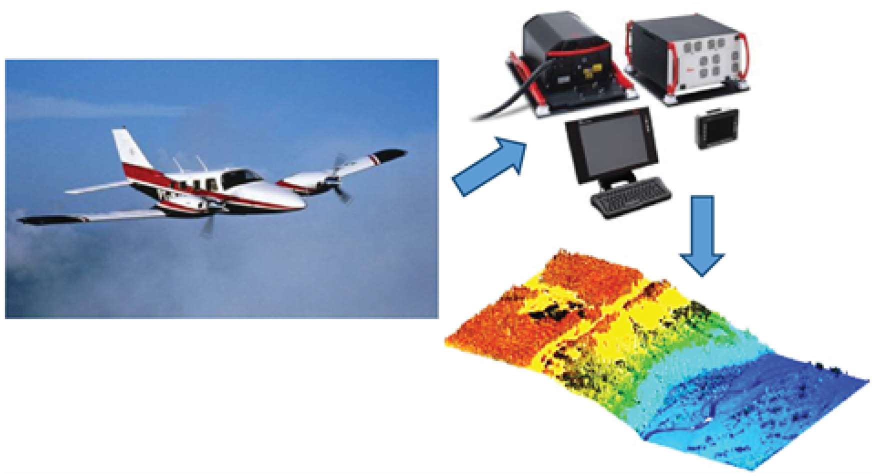
Piper Seneca V aircraft and the Leica ALS80 laser scanner.
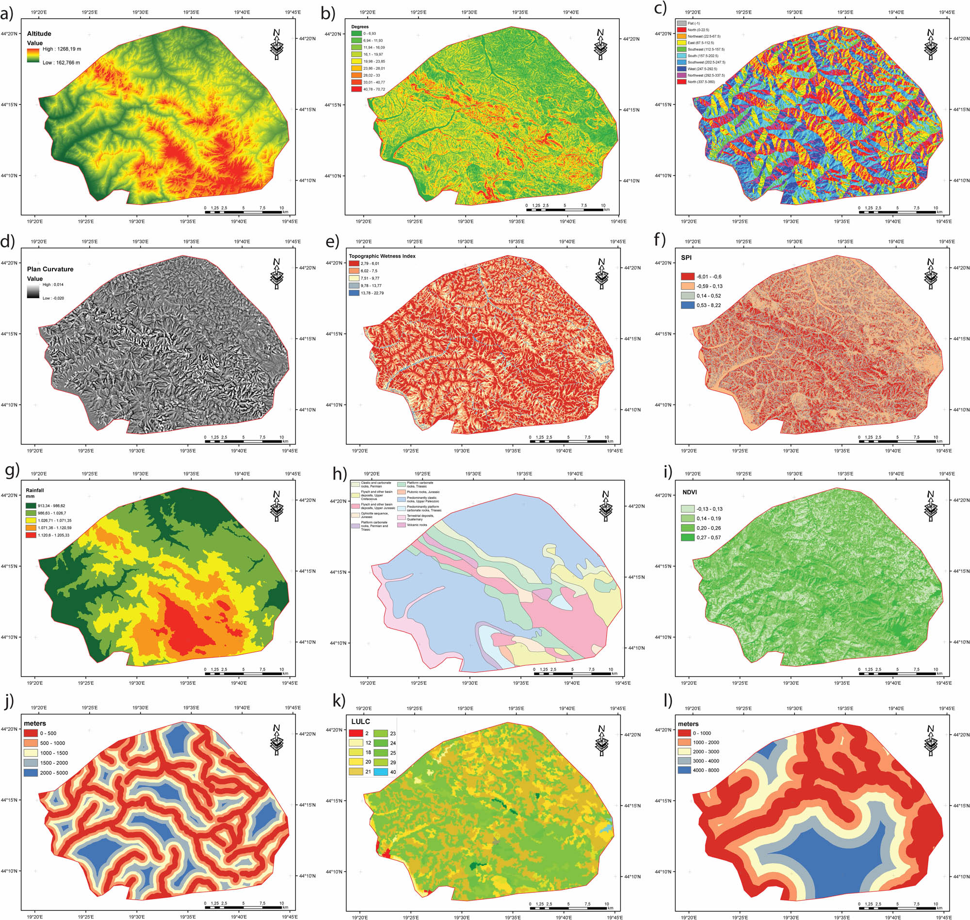
Conditioning factors related to flash floods: (a) the elevation; (b) the slope; (c) the aspect; (d) plan curvature; (e) the TWI; (f) the SPI; (g) the rainfall; (h) lithology; (i) NDVI; (j) distance to streams; (k) land use/cover; and (l) distance to roads.
The maximum magnitude of the slope change for each raster cell and its eight adjacent cells is represented by the slope angle in the DEM. The accelerated rate of particle movement and transport is impacted by the speed, kinetic energy, and tangential stresses of surface runoff, which all rise with increasing slope. In contrast, the dynamics of the process are considerably softer on gentler slopes. Long, steep slopes have a high potential for surface runoff generation, which subsequently causes gullies and furrows to form. With a range of values from 0 to 70.72°, the average terrain slope in the studied area is 16.09° (Figure 3b). Strong erosion, together with heavy soil mass washing and movement, are characteristics of this type of slope.
Aspect is likewise regarded as a secondary component that affects soil humidity and floodwater flow direction. Additionally, the slope’s curvature affects water flow because regions with zero curvature are often more vulnerable to floods than regions with positive or negative curvature values. DEM was also used to create an aspect map with nine classes – flat, north, northeast, east, southeast, south, southwest, west, and northwest – that show the direction of the terrain (Figure 3c).
The term “terrain curvature” refers to the shape of a slope and its influence on the genesis and development of erosion processes. For analysis purposes, terrain curvature is calculated using DEM. It is expressed in rad/m, but due to small values and for easier presentation of the results, it is multiplied by 100. In the horizontal plane, plan curvature represents the curvature of the contour line and is perpendicular to the direction of the greatest slope (Figure 3d). Water movement’s convergence and divergence are depicted by plan curvature. Whereas convergent slopes create areas of water and sediment buildup, divergent slopes provide runoff that influences how intense the washing and dredging operations are. Positive and negative plan curvature values are also possible. Laterally convex surfaces have positive values, whereas laterally concave surfaces have negative values. It was established that convex slopes predominate over concave ones in the studied area. These surfaces show that erosion processes (scouring, furrowing, and dredging) have begun and that surface runoff is occurring quickly.
Another crucial hydrological element of flash flood susceptibility analysis is the TWI, which captures the patterns of soil moisture associated with floodplains and measures the likelihood that water will collect at any point within a watershed due to gravity. TWI describes the effect of topography on the location and size of saturated areas of runoff generation. It is defined as [28]:
where CA is the catchment area and β is the slope angle in degrees.
Water pooling and downstream movement parameters can be thoroughly assessed thanks to the TWI, which incorporates data on flow dynamics and gravitational influence across various watershed zones (Figure 3e). In mapping flash flood susceptibility, regions with higher SPI values are more vulnerable to flash floods because of the quick erosion and channel creation that might result from strong water flow. SPI is a measure of the erosive power of flowing water based on the assumption that discharge is proportional to specific catchment area. SPI was calculated based on the formula given by Moore et al. [29]
where CA is the specific catchment’s area and β is the local slope gradient measured in degrees. Because of the extreme energy of the water flow, high SPI locations are therefore recognized as having a greater danger of abrupt and catastrophic flooding (Figure 3f).
Heavy rainfall is the primary cause of the interrelated and nearly simultaneous processes of runoff, washing, and soil erosion. Their byproducts, a vast quantity of water and sediment, then join the hydrographic network and continue to move as a two-phase fluid. The water flow and sediment transport in torrential flood waves comprise the largest portion of the overall annual water runoff and sediment transport, which is influenced by the water power in torrential processes caused by heavy rainfall. Then, soil erosion is the most severe process that degrades land resources by removing the soil’s top layer. The total annual rainfall in the different parts of the study region ranges from 913.34 to 1205.33 mm (Figure 3g).
This study also took into account a few environmental parameters, like LULC, NDVI, lithology, and distance to streams and roads. Geology is generally accepted to control the drainage pattern and the method by which rainfall is runoff. Flash flood probability is significantly influenced by lithology. The amount of water infiltration is regulated by this component, which has a significant effect on the creation of surface runoff (Figure 3h).
Additionally, NDVI is calculated by dividing the difference between the red (RED) and near-infrared reflectances by their sum, and it shows the health of the vegetation [30]. The NDVI scale goes from +1 to −1, with +1 denoting dense green-leafy vegetation and −1 denoting aquatic bodies. Vegetation has a detrimental effect on flooding, as was previously established. NDVI was calculated from the Sentinel 2 images collected on June 20, 2022. Cloud cover was 3%. This means that only a small portion of the sky, 3% to be exact, is obscured by clouds. The ArcGIS program was utilized to classify the Sentinel 2 data according to the NDVI (Figure 3i).
Flood susceptibility is significantly influenced by LULC. Different land cover types respond to floods in different ways. Densely vegetated areas, for instance, are less likely to flood because they impede water flow, but non-vegetated places, like bare lands or urban areas with impervious surfaces, accelerate rainwater runoff. Ten LULC classes are included in the CORINE land cover 2018 dataset, which we used for this analysis (Figure 3k and with a description in Table 2).
Description for the land cover/land use
| Code/Value | RGB value of vector symbology | Vector code | Description |
|---|---|---|---|
| 2 | 255,0,0 | 112 | Discontinuous urban fabric |
| 12 | 255,255,168 | 211 | Non-irrigated arable land |
| 18 | 230,230,77 | 231 | Pastures |
| 20 | 255,230,77 | 242 | Complex cultivation patterns |
| 21 | 230,204,77 | 243 | Land principally occupied by agriculture, with significant areas of natural vegetation |
| 23 | 128,255,0 | 311 | Broad-leaved forest |
| 24 | 0,166,0 | 312 | Coniferous forest |
| 25 | 77,255,0 | 313 | Mixed forest |
| 29 | 166,242,0 | 324 | Transitional woodland-shrub |
| 40 | 0,204,242 | 511 | Water courses |
Finally, using a digital topographic map and the Euclidean distance tool in ArcGIS software, distance to streams and roads data layers were created (Figure 3j and l). The scale of the used digital topographic maps is 1:25,000 (DTM25). The flash flood conditioning factors are shown in Figure 3 and Table 3, and in order to preserve uniformity pixel-by-pixel, all of the factors, including the flood map, were resampled to 10 m.
Original data of each basic environmental factor
| Factors | Classes | Number of flash flood | Percentage of flash flood (%) | Percentage of domain (%) | Ratio | Grids in the study area | Grids in flash flood |
|---|---|---|---|---|---|---|---|
| Slope angle (o) | 0–6.93 | 20 | 19.05 | 24.82 | 0.77 | 248,200 | 381 |
| 6.94–11.93 | 21 | 20.00 | 20.14 | 0.99 | 211,470 | 420 | |
| 11.94–16.09 | 16 | 15.24 | 18.17 | 0.84 | 145,360 | 244 | |
| 16.1–19.97 | 12 | 11.43 | 14.04 | 0.81 | 84,240 | 137 | |
| 19.98–23.85 | 11 | 10.48 | 7.89 | 1.33 | 43,395 | 115 | |
| 23.86–28.01 | 14 | 13.33 | 5.47 | 2.44 | 38,290 | 187 | |
| 28.02–33 | 7 | 6.67 | 4.12 | 1.62 | 14,420 | 47 | |
| 33.01–40.77 | 3 | 2.86 | 3.14 | 0.91 | 4,710 | 9 | |
| 40.78–70.72 | 1 | 0.95 | 2.21 | 0.43 | 1,105 | 1 | |
| Aspect | Flat | 4 | 3.81 | 14.29 | 0.27 | 28,580 | 15 |
| North | 16 | 15.24 | 11.38 | 1.34 | 91,040 | 244 | |
| Northeast | 15 | 14.29 | 12.24 | 1.17 | 91,800 | 214 | |
| East | 14 | 13.33 | 10.79 | 1.24 | 75,530 | 187 | |
| Southeast | 10 | 9.52 | 10.65 | 0.89 | 53,250 | 95 | |
| South | 10 | 9.52 | 9.99 | 0.95 | 49,950 | 95 | |
| Southwest | 13 | 12.38 | 10.4 | 1.19 | 67,600 | 161 | |
| West | 11 | 10.48 | 9.88 | 1.06 | 54,340 | 115 | |
| Northwest | 12 | 11.43 | 10.38 | 1.10 | 62,280 | 137 | |
| Elevation | 162.19–288.15 | 41 | 39.05 | 36.82 | 1.06 | 754,810 | 1,601 |
| 288.16–411.38 | 33 | 31.43 | 26.61 | 1.18 | 439,065 | 1,037 | |
| 411.39–641.99 | 21 | 20.00 | 17.57 | 1.14 | 184,485 | 420 | |
| 642–910.01 | 9 | 8.57 | 12.27 | 0.70 | 55,215 | 77 | |
| 910.02–1268.19 | 1 | 0.95 | 6.74 | 0.14 | 3,370 | 1 | |
| TWI | 2.79–6.01 | 15 | 14.29 | 43.38 | 0.33 | 325,350 | 214 |
| 6.02–7.5 | 22 | 20.95 | 33.05 | 0.63 | 363,550 | 461 | |
| 7.51–9.77 | 14 | 13.33 | 12.98 | 1.03 | 90,860 | 187 | |
| 9.78–13.77 | 26 | 24.76 | 0 | 644 | |||
| 13.78–22.79 | 28 | 26.67 | 10.59 | 2.52 | 148,260 | 747 | |
| Plan curvature | −2.01 to −0.6 | 24 | 22.86 | 8 | 2.86 | 96,000 | 549 |
| −0.6 to 0.13 | 28 | 26.67 | 54.47 | 0.49 | 762,580 | 747 | |
| 0.13–0.52 | 22 | 20.95 | 30.49 | 0.69 | 335,390 | 461 | |
| 0.52–1.35 | 44 | 41.90 | 7.04 | 5.95 | 154,880 | 1,844 | |
| SPI | −6.01 to −0.6 | 6 | 5.71 | 8 | 0.71 | 24,000 | 34 |
| −0.6 to 0.13 | 21 | 20.00 | 54.47 | 0.37 | 571,935 | 420 | |
| 0.13–0.52 | 34 | 32.38 | 30.49 | 1.06 | 518,330 | 1,101 | |
| 0.52–8.22 | 44 | 41.90 | 7.04 | 5.95 | 154,880 | 1,844 | |
| Lithology | Clastic rock | 6 | 5.71 | 28.07 | 0.20 | 84,210 | 34 |
| Flysch 1 | 11 | 10.48 | 2.65 | 3.95 | 14,575 | 115 | |
| Flysch 2 | 9 | 8.57 | 0.21 | 40.82 | 945 | 77 | |
| Ophiolite | 16 | 15.24 | 0.91 | 16.75 | 7,280 | 244 | |
| Carbonate rock 1 | 17 | 16.19 | 1.29 | 12.55 | 10,965 | 275 | |
| Carbonate rock 2 | 14 | 13.33 | 9.11 | 1.46 | 63,770 | 187 | |
| Plutonic rock | 10 | 9.52 | 9.04 | 1.05 | 45,200 | 95 | |
| Pred. Clastic rock | 9 | 8.57 | 5.13 | 1.67 | 23,085 | 77 | |
| Terrestrial deposits | 7 | 6.67 | 0.92 | 7.25 | 3,220 | 47 | |
| Volcanic rock | 6 | 5.71 | 0.24 | 23.81 | 720 | 34 | |
| Distance to streams (m) | 0–500 | 48 | 45.71 | 41.3 | 1.11 | 991,200 | 2,194 |
| 500–1,000 | 34 | 32.38 | 30.59 | 1.06 | 520,030 | 1,101 | |
| 1,000–1,500 | 14 | 13.33 | 16.55 | 0.81 | 115,850 | 187 | |
| 1,500–2,000 | 7 | 6.67 | 7.04 | 0.95 | 24,640 | 47 | |
| >2,000 | 2 | 1.90 | 4.53 | 0.42 | 4,530 | 4 | |
| Rainfall (mm) | 913.34–986.62 | 7 | 6.67 | 16.14 | 0.41 | 56,490 | 47 |
| 986.63–1026.7 | 12 | 11.43 | 15.29 | 0.75 | 91,740 | 137 | |
| 1026.71–1071.35 | 20 | 19.05 | 22.33 | 0.85 | 223,300 | 381 | |
| 1071.36–1120.59 | 31 | 29.52 | 24.35 | 1.21 | 377,425 | 915 | |
| 1120.6–1205.33 | 35 | 33.33 | 21.89 | 1.52 | 383,075 | 1,167 | |
| NDVI | <0.13 | 13 | 12.38 | 20.7 | 1.67 | 134,550 | 161 |
| 0.13–0.19 | 41 | 39.05 | 40.53 | 1.04 | 830,865 | 1,601 | |
| 0.19–0.26 | 36 | 34.29 | 29.34 | 0.86 | 528,120 | 1,234 | |
| >0.26 | 15 | 14.29 | 9.43 | 0.66 | 70,725 | 214 | |
| Distance to roads (m) | 0–1,000 | 21 | 20.00 | 58.57 | 0.34 | 614,985 | 420 |
| 1,000–2,000 | 24 | 22.86 | 25.55 | 0.89 | 306,600 | 549 | |
| 2,000–3,000 | 17 | 16.19 | 9.21 | 1.76 | 78,285 | 275 | |
| 3,000–4,000 | 19 | 18.10 | 4.06 | 4.46 | 38,570 | 344 | |
| >4,000 | 24 | 22.86 | 2.61 | 8.76 | 31,320 | 549 | |
| Land use/land cover | 2 | 9 | 8.57 | 1.93 | 4.44 | 8,685 | 77 |
| 12 | 12 | 11.43 | 8.28 | 1.38 | 49,680 | 137 | |
| 18 | 14 | 13.33 | 1.6 | 8.33 | 11,200 | 187 | |
| 20 | 7 | 6.67 | 25.88 | 0.26 | 90,580 | 47 | |
| 21 | 5 | 4.76 | 24.73 | 0.19 | 61,825 | 24 | |
| 23 | 21 | 20.00 | 28.64 | 0.70 | 300,720 | 420 | |
| 25 | 17 | 16.19 | 3.27 | 4.95 | 27,795 | 275 | |
| 29 | 12 | 11.43 | 3.43 | 3.33 | 20,580 | 137 | |
| 40 | 8 | 7.62 | 0.4 | 19.05 | 1,600 | 61 |
2.3 Methods
A specific methodology for assessing flash flood susceptibility was developed, considering geographic and temporal constraints. A generalized flowchart is provided in Figure 4, and the following workflows were adopted to achieve the study’s objectives:
A detailed flood inventory was prepared using WorldView 2 images, aerial images, and field investigations, focusing on historical flood locations.
Based on prior relevant research and the geo-environmental characteristics of the study area, 12 predictor variables associated with flood susceptibility were identified and subsequently prepared.
Using the well-known scikit-learn (train_test_split) Python module, the flood inventory dataset was split into 70 and 30% for training and validation, respectively.
The multicollinearity of flash flood predictor variables was tested to prevent bias in the flood mapping method, and a popular grid search technique was adopted to adjust the hyperparameters.
The current flood prediction employed three modern machine learning techniques: SVM, CART, and RF. However, only the most effective ML: RF was utilized for the mapping of future flood predictions.
The accuracy of the model’s predictions was evaluated using statistical measures such area under the curve (AUC).
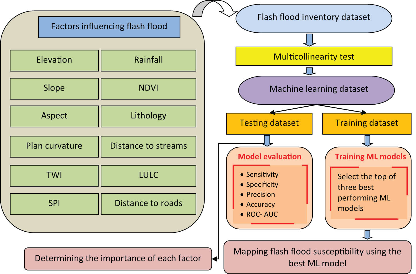
Flowchart for analysis of flash flood susceptibility based on machine learning models.
2.4 Multicollinearity analysis
Flash flood susceptibility mapping has been predicted using a variety of models based on different geoenvironmental parameters. Finding the two or more elements that have a high correlation with one another is essential among all of these conditioning components. A larger correlation between two or more conditioning elements than the model makes the evaluation less valid and automatically lowers the output result’s accuracy. Thus, the identification of these strongly correlated components is aided by multicollinearity analysis. Multicollinearity is essentially a statistical analysis of more than two variables that shows a linear relationship between them. For better outcome prediction, strong multicollinearity conditioning components must be eliminated from the models. Multicollinearity has typically been analyzed using the variance inflation factor (VIF) and tolerance (TOLERANCE) parameters. The following formula can be used to determine a multi-collinearity analysis’s TOLERANCE and VIF [31]:
where
2.5 Machine learning method used in flash flood susceptibility modeling
SVM is a supervised machine learning algorithm, and it is used in classification and regression modeling. SVM is utilized in regression and classification modeling. The model, which is founded on the optimization principle, attempts to divide the several classes by fitting a hyperplane on the training data set [32]. As far away from the nearest data points from each class as feasible is how the hyperplane is oriented. The term “support vectors” refers to these nearest positions [33]. An alternative term for a hyperplane is a decision boundary.
The RF is one supervised machine learning algorithm used in classification and regression. The method comprises a set of tree-structured classifiers. Each tree assigns a unit vote to the input vector (x) based on the most frequent class. By dividing each node into a random subset of input characteristics or predictive variables rather than the best variables, a RF classification lowers the generalization error. Additionally, an RF uses bootstrap aggregation or bagging to force the trees to grow from various subsets of training data to boost the trees’ diversity [34].
One well-known and popular decision tree algorithm is CART. The CART model is applied to problems involving both classification and regression. The binary tree is created by this paradigm by dividing the input into binary components [22]. The root node of this algorithm initially contains all of the data. Next, among the modeling traits in question, those that best distinguish the target class are chosen and added to the root node.
In this study, a set of candidate hyperparameters was chosen using grid search. Every potential combination of the chosen values is represented by a model. Performance is then assessed by testing each combination with 12-fold cross-validation. Table 4 displays the hyperparameters derived from the grid search.
Parameter showing the optimum tuning values for used models
| Model | Parameter | Best parameters |
|---|---|---|
| SVM | C | 10 |
| Gamma | Scale | |
| Kernel | Rbf | |
| RF | Number of estimators | auto |
| Max features | 200 | |
| CART | max_depth | 3 |
| min_samples_split | 5 | |
| criterion | Sqrt | |
| min_impurity_decrease | 0.0 | |
| class_weight | 1 |
2.6 Methods of validation and accuracy assessment
To measure the predictive outcome, flash flood susceptibility maps must be validated and their accuracy evaluated. Therefore, the three machine learning output findings were evaluated in this study using a variety of statistical indices and the area under the receiver operating characteristic (AUC) curves. Sensitivity (SST), specificity, positive predictive values, and negative predictive values were employed in statistical indices. Every machine learning model produced a better outcome if the value of these statistical indices was higher, and vice versa. The following formulas can be used to determine the four statistical indices that were employed in this investigation [35,36]:
where TP represents true positive, TN represents true negative, FP represents false positive, and FN represents false negative.
3 Results
3.1 Analysis of multicollinearity
VIF measures the degree to which multicollinearity increases the variance of an estimated regression coefficient. High VIF values can lead to unstable coefficient estimations, making it challenging to determine the precise effects of each independent variable on the dependent variable. To improve the prediction of results, strong multicollinearity conditioning components (VIF values more than 5) must be eliminated from the models. Taking into account the VIF and TOLERANCE limit, the multicollinearity test of 12 flash flood causative components was conducted for this analysis (Table 5). Slope (2.64) and distance to road (0.87) were linked to the highest and lowest VIF values, which ranged from roughly 0.87 to 2.64. The range for TOLERANCE was from 0.29 to 0.98. Rainfall (0.29) and aspect (0.98) were linked to the greatest and lowest TOLERANCE limit readings. Multicollinearity was not an issue with the factors chosen to estimate the risk of flash floods. Thus, the flash flood vulnerability in the current study area was modeled using all 12 explanatory variables [37,38].
Multicollinearity analysis to assess the independent variables linearity
| Variable | VIF | Tolerance |
|---|---|---|
| Elevation | 2.12 | 0.35 |
| Slope | 2.64 | 0.31 |
| Aspect | 1.09 | 0.98 |
| Plan curvature | 1.45 | 0.55 |
| TWI | 1.98 | 0.41 |
| SPI | 1.87 | 0.39 |
| Rainfall | 2.45 | 0.29 |
| Lithology | 1.47 | 0.62 |
| NDVI | 1.64 | 0.55 |
| Distance to streams | 2.01 | 0.41 |
| LULC | 1.38 | 0.65 |
| Distance to roads | 0.87 | 0.87 |
3.2 Flash flood susceptibility modeling
The percentages of each model vary, according to the analysis of the models used in this investigation. In order to detect and forecast flood-prone areas, these variances rely on the level of flood susceptibility in the region [39]. On raster maps, the flood susceptibility maps produced by each model showed values between 0.0 and 1.0. In order to preserve uniformity pixel-by-pixel, all of the conditioning factors, including the final flash flood maps, were resampled to a resolution of 10 m. Every pixel was given a unique value that represented how vulnerable it was to flooding. In particular, more flooding susceptibility is indicated by a higher number on the scale and lower flooding susceptibility is indicated by a lower value [40]. Five susceptibility classifications were created from the resulting models (Table 6 and Figure 5). For the RF model, these categories display the following percentages: 15.49, 16.04, 15.67, 23.10, and 29.70% (Figure 5c). Similar estimates were made for the SVM models very low, low, moderate, high, and extremely high percentage classes, which were 18.54, 16.74, 19.36, 21.24, and 24.12%, respectively (Figure 5a). Furthermore, the CART models’ flood-predicting percentage classes were, in order, 16.45, 14.24, 22.01, 20.78, and 26.52% (Figure 5b). In Figure 5, it can be seen that over 95% of the populated places (given in yellow) of the test area are located in high and extremely high zones susceptible to flash floods.
Areas of flash flood susceptibility class
| Models | Area | Susceptibility class | ||||
|---|---|---|---|---|---|---|
| Very low | Low | Moderate | High | Extremely high | ||
| SVM | km2 | 99.66 | 89.99 | 104.07 | 114.18 | 129.66 |
| % | 18.54 | 16.74 | 19.36 | 21.24 | 24.12 | |
| RF | km2 | 83.27 | 86.22 | 84.23 | 124.17 | 159.65 |
| % | 15.49 | 16.04 | 15.67 | 23.10 | 29.70 | |
| CART | km2 | 88.43 | 76.55 | 118.31 | 111.70 | 142.56 |
| % | 16.45 | 14.24 | 22.01 | 20.78 | 26.52 | |
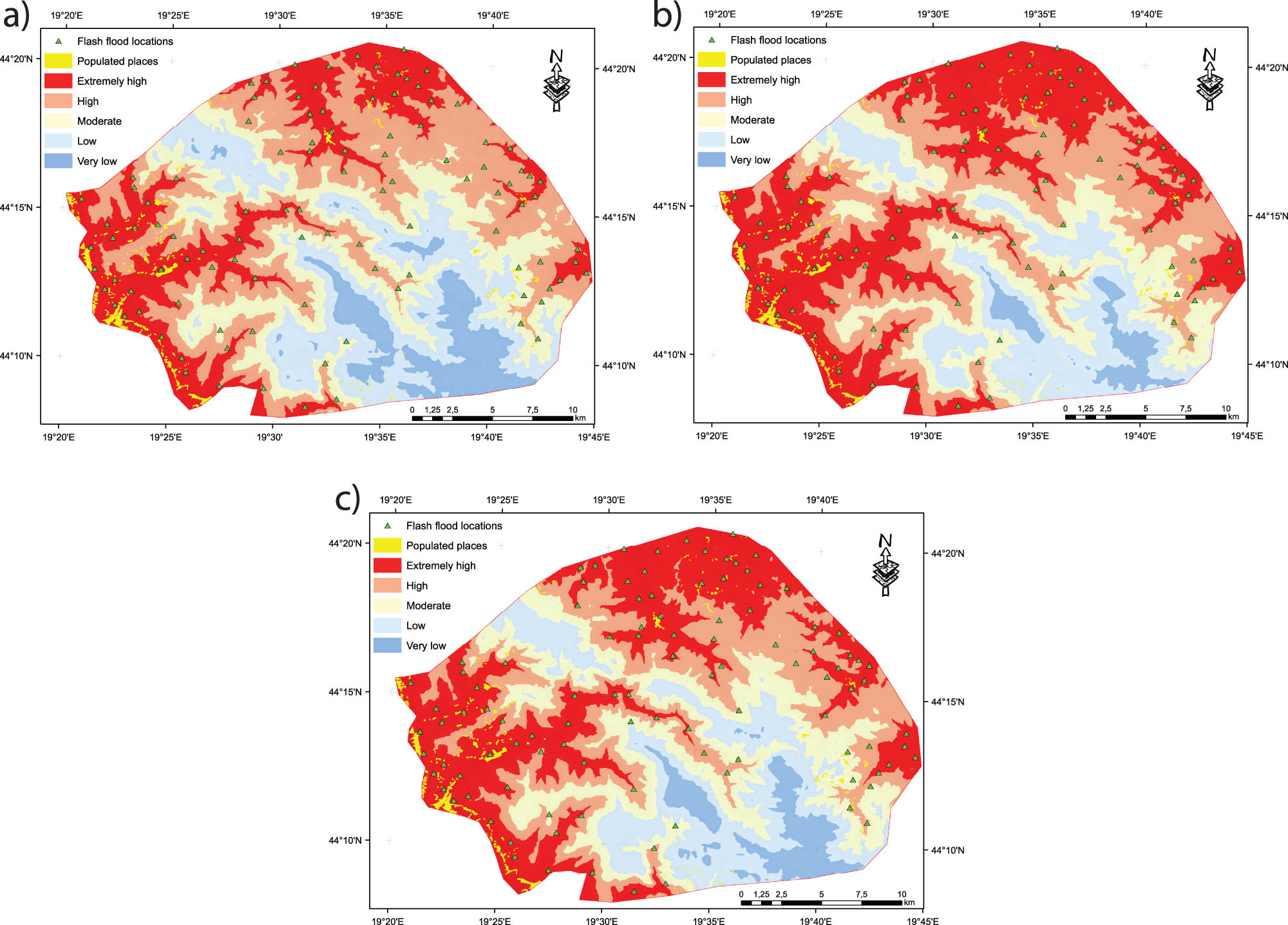
Flash flood susceptibility maps generated using machine learning models: (a) SVM, (b) CART, and (c) RF.
The Ljuboviđa basins’ flood-prone regions are primarily found in the west and north-west regions of the study area, according to the results of the percentage susceptibility classes that each model projected. These regions trace the east-west main flow of the Ljuboviđa River. A steep slope between high and low places, which makes it easier for water to concentrate during periods of severe rainfall, is what defines flood zones. Additionally, this slope makes it easier for water to flow through the bank undercutting [39,41]. Another factor contributing to floods in these locations is the absence of vegetative cover. However, the study area’s west and center sections, as well as the non-floodable zones, are distinguished by extremely dense vegetation, which prevents extended flooding in these areas.
3.3 Evaluating various ML algorithms’ performance
A crucial step in creating and refining machine learning models for various phenomena is accuracy assessment. The majority of recent machine learning research uses this curve and AUC to assess the classifiers’ performance [42,43].
An asymptotic 95% confidence interval for each of the three models used is displayed by ROC curve analysis. The CART model scored an average AUC value of 0.831 (with a confidence interval between 0.724 and 0.938), whereas the RF model was found to be the best model in this investigation with an average AUC value of 0.854 (with confidence values ranging between 0.761 and 0.947). Furthermore, the SVM model exhibited an average AUC of 0.802 (with a confidence CI of between 0.703 and 0.901), which is shown in Figure 6 and Table 7. The standard errors for the RF, CART, and SVM models were 0.047, 0.052, and 0.050, respectively (Table 7). The RF model was thus selected as the most effective model for predicting regions that are vulnerable to flooding.
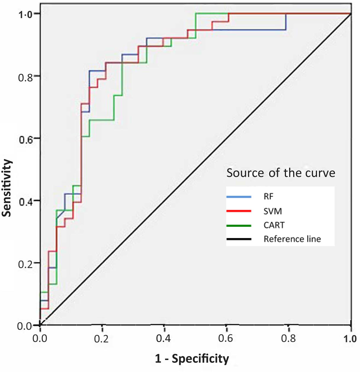
AUC of models run on the validation dataset.
AUC of models run on the validation dataset
| Models | Area | Standard error | Asymptotic significant | Asymptotic 95% confidence interval | |
|---|---|---|---|---|---|
| Lower bound | Upper bound | ||||
| RF | 0.854 | 0.047 | 0.002 | 0.761 | 0.947 |
| SVM | 0.802 | 0.052 | 0.004 | 0.703 | 0.901 |
| CART | 0.831 | 0.050 | 0.003 | 0.724 | 0.938 |
4 Discussion
As climatic events tend to intensify and land use changes constantly, the study highlights the significance of establishing a methodology for assessing areas susceptible to flash floods [20,44]. More importantly, it is necessary to develop new methodologies with new approaches in order to obtain outcomes. The investigation of three distinct machine learning techniques in this paper revealed that the RF model performs the best when mapping regions that are susceptible to flash floods [45–48].
In relation to CART, RF and SVM have simpler implications for mapping flood susceptibility. They have been examined at different geographic scales. Compared to big regions, the flood conditioning factors interaction at local scales is different [27,49,50]. Our research makes a contribution by evaluating the sub-district (local) performance of SVM. RF and CART machine learning models [51,52]. According to our research, RF was most capable of generalizing flash flood events at the local level with more statistical and spatial consistency. One possible explanation for the superior performance could be that RF tends to produce more varied classification results than SVM and CART [22,23]. Regarding AUC values, next next-mentioned studies indicate that the machine learning approach has proven reliable for flash flood modeling [53]. Machine learning algorithms have also gained popularity in flood susceptibility assessment due to their ability to process large datasets, extract complex patterns, and identify flood-prone areas. Supervised learning algorithms, such as RF, SVM, and CART, can be trained on historical flood data and integrated with LiDAR data; machine learning algorithms can provide valuable insights into flood susceptibility [22,48]. Although there are many publications discussing mapping the Republic of Serbia’s or the region’s susceptibility to flash floods, nearly all of them make use of the flash flood potential index or the geographic information system-multi-criteria decision analysis methodology [7,15,16,17,18,19].
This study identified five types of flood-prone zones: extremely high, high, moderate, low, and very low. The RF results showed that 83.27 km2 (15.49%) was a very low flood-prone area, whereas 159.65 km2 (29.70%) was an extremely high susceptible zone. Additionally, 84.23 km2 (15.67%) and 86.22 km2 (16.04%) of the area were classified as moderately and lowly susceptible, respectively, while 124.17 km2 (23.10%) was classified as highly susceptible. The total area was extremely and highly susceptible to flash floods (54.87%). These areas were the valley’s main croplands and therefore were extremely susceptible. Additionally, the majority of locations with moderate to very low flash flood susceptibility were located in hilly regions with extensive forests [54,55].
Overall, the results of this study will help future research with more thorough analyses and allow policymakers and planners to implement sustainable measures for improving local communities’ preparedness against flash floods. However, each machine learning model has limitations because of its subjectivity in choosing flood conditioning factors, training samples, and evaluation metrics.
The occurrence of flash floods is the result of several natural processes in torrential basins that represent components of the runoff cycle, as part of the global hydrological cycle. Specific and variable characteristics of climate and relief, terrain geology, pedological and vegetation cover, but also changes in socioeconomic conditions, such as population migration or land use, create a wide range of conditions and factors for the occurrence of flash floods in Serbia. More than 12,000 flash floods have been registered on the territory of Serbia, so flash floods are the most frequent phenomenon in the arsenal of so-called “natural risks.” Extreme rain episodes are the main driver of the process of genesis of surface runoff and soil erosion, which are directly and closely related. They take place almost simultaneously and their products, a huge amount of water and sediment, enter the hydrographic network and continue their movement as a two-phase fluid. The occurrence of extreme flows on watercourses depends on a whole series of factors that condition and supplements each other. Slopes without vegetation, with a degraded surface soil layer, are predisposed to surface runoff and erosion. The reduction of areas under forest vegetation, soil degradation, inappropriate land cultivation techniques, and urbanization are just some of the negative human influences that contribute to the occurrence of flash floods, so that former 100-year flows become 20-year flows.
In addition to the mentioned climatic factors and relief, the characteristics of land and vegetation cover and socio-economic conditions also play an important role in the occurrence of flash floods, as a catalyst for changes in the way space is used and population migration. The occurrence of flash floods in the territory of the Republic of Serbia is primarily related to hilly and mountainous areas that are threatened by intense erosion processes, but they also occur in valley sections of torrential flows. One of the basic factors for the generation of flash floods is the specific structure of the areas (way of using space) in the basin. Inappropriate land use practices, excessive exploitation of land and forest resources, as well as urbanization processes, lead to the intensification of erosion processes, which consequently result in degradation and reduction of the infiltration-retention capacity of the soil. Such modified environmental conditions lead to the intensification of rapid surface runoff on the slopes of the basins and the generation of flash floods in the hydrographic network.
5 Conclusion
In this study, three distinct machine learning models based on the high-resolution LiDAR-derived DEM were used to study flash flood susceptibility. The use of machine learning in hydrologic modeling for flood forecasting has increased dramatically in recent years, as seen by the substantial increase in the number of scholarly publications in this area. A significant factor in the creation of machine learning-based models has been the advancement of technology as well as the growing frequency and severity of hydrometeorological events.
A wide range of conditions and factors contribute to the occurrence of flash floods in Serbia, including changing socioeconomic conditions like land use patterns or population migration, as well as specific and variable features of the climate and relief, terrain geology, soil, and vegetation cover [11,45]. The dominance of those conditions and factors that encourage the occurrence of flash floods determines how frequently they occur. While the lower, typically populated terrain of the same basins is frequently much more at risk from flood waves, the genesis of flash flood waters is associated with hilly and mountainous locations [46,56].
Prediction robustness can be greatly impacted by limitations in terrain characteristics, climate prediction, or previous flood data [21,57,58]. Adding comprehensive flash flood data, like decadal flood data, could improve datasets and the results of model training. This study may have been more accurate if a higher resolution DTM had been used in place of the existing DEM. LiDAR is the best data source for creating DTMs and other flood modeling applications. The LiDAR-based DTM produced better drainage delineation, according to the results, which improved the accuracy of flood susceptibility mapping [59]. Comparing the LiDAR-based DTM to the other DTMs, the results show that it performed better in mapping susceptibility and describing local drainage patterns. In conclusion, high-resolution DEMs play a significant role in creating precise and trustworthy maps of the incidence of flash floods. The use of these maps aids in the management and reduction of disaster risk, particularly in determining which regions should be given priority in order to provide suitable flood risk management strategies that will be implemented to prevent flood disasters. Prior research has suggested that LiDAR-derived DEMs increase the precision of flood parameters; as a result, they can aid in the creation of superior flood risk and hazard mapping [3,10,11].
Since machine learning algorithms trained on specific datasets may not generalize across a variety of geographical or climatic conditions, restricting their usefulness outside the study area in hilly regions of western Serbia, future research should take these difficulties into account [60,61]. Using higher-resolution climate data and adding future temperature and LULC cover data to improve flood forecasts are two ways to address these concerns. Significant computer power, technical know-how, and ongoing funding are needed to deploy machine learning-based flood prediction systems on official websites. However, the viability and durability of this strategy may be impacted by resource limitations in data collecting, model training, or operational deployment. To improve the validity and relevance of results and suggestions for controlling flash floods in the area, further research should address these constraints [51,52].
The prediction of the risk of flash flooding during extreme rainy episodes allows spatial planners in threatened river basins to make rational decisions in order to prevent and minimize possible negative impacts. The models help in the process of identifying threatened regions and watersheds, from the aspect of SST to the occurrence of intense erosion processes and flash floods.
Acknowledgments
This study was supported by the project of the Ministry of Defense 1.18.2025 – “Development of a primary standard for length and angle in laboratory conditions.”
-
Funding information: This research received no external funding that has supported the work.
-
Author contributions: Conceptualisation and methodology: S. D. and D. Dj.; formal analysis: M. S., S. D., and Z. M.; GIS software and mapping: S. D. and M.S.; technical editing: S.D. and Z. M.; supervision: D. Dj. All authors discussed the results and contributed to the final manuscript. All authors have read and agreed to the published version of the manuscript.
-
Conflict of interest: The authors state no conflict of interest.
-
Data availability statement: The datasets used and/or analyzed during the current study are available from the corresponding author upon reasonable request.
References
[1] Gigović L, Pamučar D, Bajić Z, Drobnjak S. Application of GIS-interval rough AHP methodology for flood hazard mapping in Urban areas. Water (Switzerland). 2017;9(6):360. 10.3390/w9060360.Search in Google Scholar
[2] Wang Y, Hong H, Chen W, Li S, Pamučar D, Gigović L, et al. A hybrid GIS multi-criteria decision-making method for flood susceptibility mapping at Shangyou, China. Remote Sens (Basel). 2019;11:62.10.3390/rs11010062Search in Google Scholar
[3] Costache R, Tien Bui D. Spatial prediction of flood potential using new ensembles of bivariate statistics and artificial intelligence: A case study at the Putna river catchment of Romania. Sci Total Environ. 2019;691:1098–118. 10.1016/J.SCITOTENV.2019.07.197.Search in Google Scholar PubMed
[4] Dragićević S, Kostadinov S, Novković I, Momirović N, Langović M, Stefanović T, et al. Assessment of soil erosion and torrential flood susceptibility: Case Study – Timok River Basin, Serbia. In: The lower Danube river: Hydro-environmental issues and sustainability. Cham: Springer International Publishing; 2022. p. 357–80. 10.1007/978-3-031-03865-5_12.Search in Google Scholar
[5] Durlević U, Novković I, Lukić T, Valjarević A, Samardzić I, Krstić F, et al. Multihazard susceptibility assessment: A case study – Municipality of Štrpce (Southern Serbia). Open Geosci. 2021;13:1414–31. 10.1515/GEO-2020-0314/ASSET/GRAPHIC/J_GEO-2020-0314_FIG_011.JPG.Search in Google Scholar
[6] Lazarević K, Todosijević M, Vulević T, Polovina S, Momirović N, Caković M. Determination of flash flood hazard areas in the Likodra watershed. Water. 2023;15:2698. 10.3390/W15152698.Search in Google Scholar
[7] Durlević U. Assessment of torrential flood and landslide susceptibility of terrain: Case study – Mlava River Basin (Serbia). Glas Srpskog Geografskog Drustva. 2021;101:49–75. 10.2298/GSGD2101049D.Search in Google Scholar
[8] Zhang C, Bi W. Global experiences in flood management – perspectives through ICFM Webinar Series. Proc IAHS. 2024;386:307–12. 10.5194/PIAHS-386-307-2024.Search in Google Scholar
[9] Taherizadeh M, Niknam A, Nguyen-Huy T, Mezősi G, Sarli R. Flash flood-risk areas zoning using integration of decision-making trial and evaluation laboratory, GIS-based analytic network process and satellite-derived information. Nat Hazards. 2023;118:2309–35. 10.1007/s11069-023-06089-5.Search in Google Scholar
[10] Vennari C, Parise M, Santangelo N, Santo A. A database on flash flood events in Campania, southern Italy, with an evaluation of their spatial and temporal distribution. Nat Hazards Earth Syst Sci. 2016;16:2485–500. 10.5194/NHESS-16-2485-2016.Search in Google Scholar
[11] Janizadeh S, Avand M, Jaafari A, Van Phong T, Bayat M, Ahmadisharaf E, et al. Prediction success of machine learning methods for flash flood susceptibility mapping in the Tafresh Watershed, Iran. Sustainability. 2019;11:5426. 10.3390/SU11195426.Search in Google Scholar
[12] Costache R, Pham QB, Sharifi E, Linh NTT, Abba SI, Vojtek M, et al. Flash-flood susceptibility assessment using multi-criteria decision making and machine learning supported by remote sensing and GIS techniques. Remote Sens. 2019;12:106. 10.3390/RS12010106.Search in Google Scholar
[13] Petrovic A. Challenges of torrential flood risk management in Serbia. J Geogr Inst Jovan Cvijic, SASA. 2015;65:131–43. 10.2298/IJGI1502131P.Search in Google Scholar
[14] Petrović AM, Leščešen I, Radevski I. Unveiling torrential flood dynamics: a comprehensive study of spatio-temporal patterns in the Šumadija Region, Serbia. Water. 2024;16:991. 10.3390/W16070991.Search in Google Scholar
[15] Aleksova B, Milevski I, Mijalov R, Marković SB, Cvetković VM, Lukić T. Assessing risk-prone areas in the Kratovska Reka catchment (North Macedonia) by integrating advanced geospatial analytics and flash flood potential index. Open Geosci. 2024;16(1):20220684. 10.1515/geo-2022-0684.Search in Google Scholar
[16] Aleksova B, Milevski I, Dragićević S, Lukić T. GIS-based integrated multi-hazard vulnerability assessment in Makedonska Kamenica Municipality, North Macedonia. Atmosphere. 2024;15:774. 10.3390/ATMOS15070774.Search in Google Scholar
[17] Sabljić L, Pavić D, Savić S, Bajić D. Extreme precipitations and their influence on the River flood Hazards: A case study of the Sana River Basin in Bosnia and Herzegovina. Geogr Pannonica. 2023;27:184–98. 10.5937/GP27-45600.Search in Google Scholar
[18] Lovrić N, Tošić R, Dragićević S, Novković I. Assessment of torrential flood susceptibility: Case study – Ukrina River Basin (B&H). Glas Srpskog Geografskog Drustva. 2019;99:1–16. 10.2298/GSGD1902001L.Search in Google Scholar
[19] Vujović F, Valjarević A, Durlević U, Morar C, Grama V, Spalević V, et al. A comparison of the AHP and BWM models for the flash flood susceptibility assessment: a case study of the Ibar River Basin in Montenegro. Water. 2025;17:844. 10.3390/W17060844.Search in Google Scholar
[20] Bui DT, Ngo PTT, Pham TD, Jaafari A, Minh NQ, Hoa PV, et al. A novel hybrid approach based on a swarm intelligence optimized extreme learning machine for flash flood susceptibility mapping. Catena (Amst). 2019;179:184–96. 10.1016/J.CATENA.2019.04.009.Search in Google Scholar
[21] Yin Y, Zhang X, Guan Z, Chen Y, Liu C, Yang T. Flash flood susceptibility mapping based on catchments using an improved Blending machine learning approach. Hydrol Res. 2023;54:557–79. 10.2166/NH.2023.139.Search in Google Scholar
[22] Ahmadlou M, Ebrahimian Ghajari Y, Karimi M. Enhanced classification and regression tree (CART) by genetic algorithm (GA) and grid search (GS) for flood susceptibility mapping and assessment. Geocarto Int. 2022;37:13638–57. 10.1080/10106049.2022.2082550.Search in Google Scholar
[23] Sheikh Z, Zolfaghari AA, Raeesi M, Soltani A. Enhancing flash flood susceptibility modeling in arid regions: integrating digital soil mapping and machine learning algorithms. Environ Earth Sci. 2025;84:170. 10.1007/S12665-025-12140-4.Search in Google Scholar
[24] Gigović L, Pourghasemi HR, Drobnjak S, Bai S. Testing a new ensemble model based on SVM and random forest in forest fire susceptibility assessment and its mapping in Serbia’s Tara National Park. Forests. 2019;10(5):408. 10.3390/f10050408.Search in Google Scholar
[25] Petrović AM, Kostadinov S, Ristić R, Novković I, Radevski I. The reconstruction of the great 2020 torrential flood in Western Serbia. Nat Hazards. 2023;118:1673–88. 10.1007/S11069-023-06066-Y/METRICS.Search in Google Scholar
[26] Republic Hydrometeorological Service of Serbia, Kneza Višeslava 66, Belgrade, Republic Serbia. n.d. https://www.hidmet.gov.rs/eng/download/index.php (accessed April 10, 2025).Search in Google Scholar
[27] Tsubaki R, Fujita I. Unstructured grid generation using LiDAR data for urban flood inundation modelling. Hydrol Processes: Int J. 2010;24:1404–20. 10.1002/HYP.7608.Search in Google Scholar
[28] Moore ID, Grayson RB, Ladson AR. Digital terrain modelling: a review of hydrological, geomorphological, and biological applications. Hydrol Process. 1991;5:3–30. 10.1002/HYP.3360050103.Search in Google Scholar
[29] Moore ID, Gessler PE, Nielsen GA, Peterson GA. Soil attribute prediction using terrain analysis. Soil Sci Soc Am J. 1993;57:443–52. 10.2136/SSSAJ1993.03615995005700020026X.Search in Google Scholar
[30] Rouse JW, Haas RH, Scheel JA, Deering DW. Monitoring vegetation systems in the great plains with ERTS. Third Earth Resources Technology Satellite-1 Symposium. Volume 1: Technical Presentations, section A. 1974. p. 48–62.Search in Google Scholar
[31] Kyriazos T, Poga M, Kyriazos T, Poga M. Dealing with multicollinearity in factor analysis: the problem, detections, and solutions. Open J Stat. 2023;13:404–24. 10.4236/OJS.2023.133020.Search in Google Scholar
[32] Liu J, Wang J, Xiong J, Cheng W, Sun H, Yong Z, et al. Hybrid models incorporating bivariate statistics and machine learning methods for flash flood susceptibility assessment based on remote sensing datasets. Remote Sens. 2021;13:4945. 10.3390/RS13234945.Search in Google Scholar
[33] Sakr GE, Elhajj IH, Abou-Saad Huijer H. Support vector machines to define and detect agitation transition. IEEE Trans Affect Comput. 2010;1:98–108. 10.1109/T-AFFC.2010.2.Search in Google Scholar
[34] Breiman L. Random forests. Mach Learn. 2001;45:5–32. 10.1023/A:1010933404324.Search in Google Scholar
[35] Pham BT, Luu C, Van Dao D, Van Phong T, Nguyen HD, Van Le H, et al. Flood risk assessment using deep learning integrated with multi-criteria decision analysis. Knowl Based Syst. 2021;219:106899. 10.1016/J.KNOSYS.2021.106899.Search in Google Scholar
[36] Zhu Z, Zhang Y. Flood disaster risk assessment based on random forest algorithm. Neural Comput Appl. 2022;34:3443–55. 10.1007/S00521-021-05757-6.Search in Google Scholar
[37] Khosravi K, Pham BT, Chapi K, Shirzadi A, Shahabi H, Revhaug I, et al. A comparative assessment of decision trees algorithms for flash flood susceptibility modeling at Haraz watershed, northern Iran. Sci Total Environ. 2018;627:744–55. 10.1016/J.SCITOTENV.2018.01.266.Search in Google Scholar
[38] Xiong J, Ye C, Cheng W, Guo L, Zhou C, Zhang X. The spatiotemporal distribution of flash floods and analysis of partition driving forces in Yunnan Province. Sustainability (Switzerland). 2019;11(10):2926. 10.3390/SU11102926.Search in Google Scholar
[39] Tehrany MS, Pradhan B, Jebur MN. Flood susceptibility mapping using a novel ensemble weights-of-evidence and support vector machine models in GIS. J Hydrol (Amst). 2014;512:332–43. 10.1016/J.JHYDROL.2014.03.008.Search in Google Scholar
[40] Youssef AM, Pradhan B, Hassan AM. Flash flood risk estimation along the St. Katherine road, southern Sinai, Egypt using GIS based morphometry and satellite imagery. Environ Earth Sci. 2011;62:611–23. 10.1007/S12665-010-0551-1.Search in Google Scholar
[41] Minea G. Assessment of the flash flood potential of Bâsca river catchment (Romania) based on physiographic factors. Cent Eur J Geosci. 2013;5:344–53. 10.2478/S13533-012-0137-4.Search in Google Scholar
[42] Tincu R, Lazar G, Lazar I. Modified flash flood potential index in order to estimate areas with predisposition to water accumulation. Open Geosci. 2018;10:593–606. 10.1515/GEO-2018-0047.Search in Google Scholar
[43] Costache R, Ngo PTT, Bui DT. Novel ensembles of deep learning neural network and statistical learning for flash-flood susceptibility mapping. Water. 2020;12:1549. 10.3390/W12061549.Search in Google Scholar
[44] Towfiqul Islam ARM, Talukdar S, Mahato S, Kundu S, Eibek KU, Pham QB, et al. Flood susceptibility modelling using advanced ensemble machine learning models. Geosci Front. 2021;12(3):101075. 10.1016/j.gsf.2020.09.006.Search in Google Scholar
[45] Hosseini FS, Choubin B, Mosavi A, Nabipour N, Shamshirband S, Darabi H, et al. Flash-flood hazard assessment using ensembles and Bayesian-based machine learning models: Application of the simulated annealing feature selection method. Sci Total Environ. 2020;711:135161. 10.1016/j.scitotenv.2019.135161.Search in Google Scholar PubMed
[46] Elmahdy S, Ali T, Mohamed M. Flash flood susceptibility modeling and magnitude index using machine learning and geohydrological models: a modified hybrid approach. Remote Sens. 2020;12:2695. 10.3390/RS12172695.Search in Google Scholar
[47] Arabameri A, Seyed Danesh A, Santosh M, Cerda A, Chandra Pal S, Ghorbanzadeh O, et al. Flood susceptibility mapping using meta-heuristic algorithms. Geomatics Nat Hazards Risk. 2022;13:949–74. 10.1080/19475705.2022.2060138.Search in Google Scholar
[48] Ilia I, Tsangaratos P, Tzampoglou P, Chen W, Hong H. Flash flood susceptibility mapping using stacking ensemble machine learning models. Geocarto Int. 2022;37:15010–36. 10.1080/10106049.2022.2093990;WGROUP:STRING:PUBLICATION.Search in Google Scholar
[49] Abedi R, Costache R, Shafizadeh-Moghadam H, Pham QB. Flash-flood susceptibility mapping based on XGBoost, random forest and boosted regression trees. Geocarto Int. 2022;37:5479–96. 10.1080/10106049.2021.1920636.Search in Google Scholar
[50] Prasad P, Loveson VJ, Das B, Kotha M. Novel ensemble machine learning models in flood susceptibility mapping. Geocarto Int. 2022;37:4571–93. 10.1080/10106049.2021.1892209.Search in Google Scholar
[51] Hitouri S, Mohajane M, Lahsaini M, Ali SA, Setargie TA, Tripathi G, et al. Flood susceptibility mapping using SAR data and machine learning algorithms in a small watershed in Northwestern Morocco. Remote Sens. 2024;16:858. 10.3390/RS16050858.Search in Google Scholar
[52] Band SS, Janizadeh S, Pal SC, Saha A, Chakrabortty R, Melesse AM, et al. Flash flood susceptibility modeling using new approaches of hybrid and ensemble tree-based machine learning algorithms. Remote Sens. 2020;12:3568. 10.3390/RS12213568.Search in Google Scholar
[53] Tehrany MS, Jones S, Shabani F. Identifying the essential flood conditioning factors for flood prone area mapping using machine learning techniques. Catena (Amst). 2019;175:174–92. 10.1016/J.CATENA.2018.12.011.Search in Google Scholar
[54] Pham BT, Avand M, Janizadeh S, Van Phong T, Al-Ansari N, Ho LS, et al. GIS based hybrid computational approaches for flash flood susceptibility assessment. Water. 2020;12:683. 10.3390/W12030683.Search in Google Scholar
[55] He F, Liu S, Mo X, Wang Z. Interpretable flash flood susceptibility mapping in Yarlung Tsangpo River Basin using H2O Auto-ML. Sci Rep. 2025;15:1702. 10.1038/S41598-024-84655-Y;SUBJMETA=242,4111,704;KWRD=HYDROLOGY,NATURAL+HAZARDS.Search in Google Scholar
[56] Elkhrachy I. Flash flood hazard mapping using satellite images and GIS tools: a case study of Najran City, Kingdom of Saudi Arabia (KSA). Egypt J Remote Sens Space Sci. 2015;18:261–78. 10.1016/J.EJRS.2015.06.007.Search in Google Scholar
[57] Abdelkareem M. Targeting flash flood potential areas using remotely sensed data and GIS techniques. Nat Hazards. 2017;85:19–37. 10.1007/S11069-016-2556-X.Search in Google Scholar
[58] Arabameri A, Saha S, Chen W, Roy J, Pradhan B, Bui DT. Flash flood susceptibility modelling using functional tree and hybrid ensemble techniques. J Hydrol (Amst). 2020;587:125007. 10.1016/J.JHYDROL.2020.125007.Search in Google Scholar
[59] Liu X, Zhang Z, McDougall K. Characteristic analysis of a flash flood-affected creek catchment using LiDAR-derived DEM. MODSIM 2011 – 19th International Congress on Modelling and Simulation – Sustaining Our Future: Understanding and Living with Uncertainty. 2011. p. 2409–15. 10.36334/MODSIM.2011.E14.LIU.Search in Google Scholar
[60] Costache R. Flash-Flood Potential assessment in the upper and middle sector of Prahova river catchment (Romania). A comparative approach between four hybrid models. Sci Total Environ. 2019;659:1115–34. 10.1016/J.SCITOTENV.2018.12.397.Search in Google Scholar
[61] Costache R. Flood susceptibility assessment by using bivariate statistics and machine learning models – a useful tool for flood risk management. Water Resour Manag. 2019;33:3239–56. 10.1007/S11269-019-02301-Z.Search in Google Scholar
© 2025 the author(s), published by De Gruyter
This work is licensed under the Creative Commons Attribution 4.0 International License.
Articles in the same Issue
- Ionization hotspots near waterfalls in Eastern Serbia’s Stara Planina Mountain
- Research Articles
- Seismic response and damage model analysis of rocky slopes with weak interlayers
- Multi-scenario simulation and eco-environmental effect analysis of “Production–Living–Ecological space” based on PLUS model: A case study of Anyang City
- Remote sensing estimation of chlorophyll content in rape leaves in Weibei dryland region of China
- GIS-based frequency ratio and Shannon entropy modeling for landslide susceptibility mapping: A case study in Kundah Taluk, Nilgiris District, India
- Natural gas origin and accumulation of the Changxing–Feixianguan Formation in the Puguang area, China
- Spatial variations of shear-wave velocity anomaly derived from Love wave ambient noise seismic tomography along Lembang Fault (West Java, Indonesia)
- Evaluation of cumulative rainfall and rainfall event–duration threshold based on triggering and non-triggering rainfalls: Northern Thailand case
- Pixel and region-oriented classification of Sentinel-2 imagery to assess LULC dynamics and their climate impact in Nowshera, Pakistan
- The use of radar-optical remote sensing data and geographic information system–analytical hierarchy process–multicriteria decision analysis techniques for revealing groundwater recharge prospective zones in arid-semi arid lands
- Effect of pore throats on the reservoir quality of tight sandstone: A case study of the Yanchang Formation in the Zhidan area, Ordos Basin
- Hydroelectric simulation of the phreatic water response of mining cracked soil based on microbial solidification
- Spatial-temporal evolution of habitat quality in tropical monsoon climate region based on “pattern–process–quality” – a case study of Cambodia
- Early Permian to Middle Triassic Formation petroleum potentials of Sydney Basin, Australia: A geochemical analysis
- Micro-mechanism analysis of Zhongchuan loess liquefaction disaster induced by Jishishan M6.2 earthquake in 2023
- Prediction method of S-wave velocities in tight sandstone reservoirs – a case study of CO2 geological storage area in Ordos Basin
- Ecological restoration in valley area of semiarid region damaged by shallow buried coal seam mining
- Hydrocarbon-generating characteristics of Xujiahe coal-bearing source rocks in the continuous sedimentary environment of the Southwest Sichuan
- Hazard analysis of future surface displacements on active faults based on the recurrence interval of strong earthquakes
- Structural characterization of the Zalm district, West Saudi Arabia, using aeromagnetic data: An approach for gold mineral exploration
- Research on the variation in the Shields curve of silt initiation
- Reuse of agricultural drainage water and wastewater for crop irrigation in southeastern Algeria
- Assessing the effectiveness of utilizing low-cost inertial measurement unit sensors for producing as-built plans
- Analysis of the formation process of a natural fertilizer in the loess area
- Machine learning methods for landslide mapping studies: A comparative study of SVM and RF algorithms in the Oued Aoulai watershed (Morocco)
- Chemical dissolution and the source of salt efflorescence in weathering of sandstone cultural relics
- Molecular simulation of methane adsorption capacity in transitional shale – a case study of Longtan Formation shale in Southern Sichuan Basin, SW China
- Evolution characteristics of extreme maximum temperature events in Central China and adaptation strategies under different future warming scenarios
- Estimating Bowen ratio in local environment based on satellite imagery
- 3D fusion modeling of multi-scale geological structures based on subdivision-NURBS surfaces and stratigraphic sequence formalization
- Comparative analysis of machine learning algorithms in Google Earth Engine for urban land use dynamics in rapidly urbanizing South Asian cities
- Study on the mechanism of plant root influence on soil properties in expansive soil areas
- Simulation of seismic hazard parameters and earthquakes source mechanisms along the Red Sea rift, western Saudi Arabia
- Tectonics vs sedimentation in foredeep basins: A tale from the Oligo-Miocene Monte Falterona Formation (Northern Apennines, Italy)
- Investigation of landslide areas in Tokat-Almus road between Bakımlı-Almus by the PS-InSAR method (Türkiye)
- Predicting coastal variations in non-storm conditions with machine learning
- Cross-dimensional adaptivity research on a 3D earth observation data cube model
- Geochronology and geochemistry of late Paleozoic volcanic rocks in eastern Inner Mongolia and their geological significance
- Spatial and temporal evolution of land use and habitat quality in arid regions – a case of Northwest China
- Ground-penetrating radar imaging of subsurface karst features controlling water leakage across Wadi Namar dam, south Riyadh, Saudi Arabia
- Rayleigh wave dispersion inversion via modified sine cosine algorithm: Application to Hangzhou, China passive surface wave data
- Fractal insights into permeability control by pore structure in tight sandstone reservoirs, Heshui area, Ordos Basin
- Debris flow hazard characteristic and mitigation in Yusitong Gully, Hengduan Mountainous Region
- Research on community characteristics of vegetation restoration in hilly power engineering based on multi temporal remote sensing technology
- Identification of radial drainage networks based on topographic and geometric features
- Trace elements and melt inclusion in zircon within the Qunji porphyry Cu deposit: Application to the metallogenic potential of the reduced magma-hydrothermal system
- Pore, fracture characteristics and diagenetic evolution of medium-maturity marine shales from the Silurian Longmaxi Formation, NE Sichuan Basin, China
- Study of the earthquakes source parameters, site response, and path attenuation using P and S-waves spectral inversion, Aswan region, south Egypt
- Source of contamination and assessment of potential health risks of potentially toxic metal(loid)s in agricultural soil from Al Lith, Saudi Arabia
- Regional spatiotemporal evolution and influencing factors of rural construction areas in the Nanxi River Basin via GIS
- An efficient network for object detection in scale-imbalanced remote sensing images
- Effect of microscopic pore–throat structure heterogeneity on waterflooding seepage characteristics of tight sandstone reservoirs
- Environmental health risk assessment of Zn, Cd, Pb, Fe, and Co in coastal sediments of the southeastern Gulf of Aqaba
- A modified Hoek–Brown model considering softening effects and its applications
- Evaluation of engineering properties of soil for sustainable urban development
- The spatio-temporal characteristics and influencing factors of sustainable development in China’s provincial areas
- Application of a mixed additive and multiplicative random error model to generate DTM products from LiDAR data
- Gold vein mineralogy and oxygen isotopes of Wadi Abu Khusheiba, Jordan
- Prediction of surface deformation time series in closed mines based on LSTM and optimization algorithms
- 2D–3D Geological features collaborative identification of surrounding rock structural planes in hydraulic adit based on OC-AINet
- Spatiotemporal patterns and drivers of Chl-a in Chinese lakes between 1986 and 2023
- Land use classification through fusion of remote sensing images and multi-source data
- Nexus between renewable energy, technological innovation, and carbon dioxide emissions in Saudi Arabia
- Analysis of the spillover effects of green organic transformation on sustainable development in ethnic regions’ agriculture and animal husbandry
- Factors impacting spatial distribution of black and odorous water bodies in Hebei
- Large-scale shaking table tests on the liquefaction and deformation responses of an ultra-deep overburden
- Impacts of climate change and sea-level rise on the coastal geological environment of Quang Nam province, Vietnam
- Reservoir characterization and exploration potential of shale reservoir near denudation area: A case study of Ordovician–Silurian marine shale, China
- Seismic prediction of Permian volcanic rock reservoirs in Southwest Sichuan Basin
- Application of CBERS-04 IRS data to land surface temperature inversion: A case study based on Minqin arid area
- Geological characteristics and prospecting direction of Sanjiaoding gold mine in Saishiteng area
- Research on the deformation prediction model of surrounding rock based on SSA-VMD-GRU
- Geochronology, geochemical characteristics, and tectonic significance of the granites, Menghewula, Southern Great Xing’an range
- Hazard classification of active faults in Yunnan base on probabilistic seismic hazard assessment
- Characteristics analysis of hydrate reservoirs with different geological structures developed by vertical well depressurization
- Estimating the travel distance of channelized rock avalanches using genetic programming method
- Landscape preferences of hikers in Three Parallel Rivers Region and its adjacent regions by content analysis of user-generated photography
- New age constraints of the LGM onset in the Bohemian Forest – Central Europe
- Characteristics of geological evolution based on the multifractal singularity theory: A case study of Heyu granite and Mesozoic tectonics
- Soil water content and longitudinal microbiota distribution in disturbed areas of tower foundations of power transmission and transformation projects
- Oil accumulation process of the Kongdian reservoir in the deep subsag zone of the Cangdong Sag, Bohai Bay Basin, China
- Investigation of velocity profile in rock–ice avalanche by particle image velocimetry measurement
- Optimizing 3D seismic survey geometries using ray tracing and illumination modeling: A case study from Penobscot field
- Sedimentology of the Phra That and Pha Daeng Formations: A preliminary evaluation of geological CO2 storage potential in the Lampang Basin, Thailand
- Improved classification algorithm for hyperspectral remote sensing images based on the hybrid spectral network model
- Map analysis of soil erodibility rates and gully erosion sites in Anambra State, South Eastern Nigeria
- Identification and driving mechanism of land use conflict in China’s South-North transition zone: A case study of Huaihe River Basin
- Evaluation of the impact of land-use change on earthquake risk distribution in different periods: An empirical analysis from Sichuan Province
- A test site case study on the long-term behavior of geotextile tubes
- An experimental investigation into carbon dioxide flooding and rock dissolution in low-permeability reservoirs of the South China Sea
- Detection and semi-quantitative analysis of naphthenic acids in coal and gangue from mining areas in China
- Comparative effects of olivine and sand on KOH-treated clayey soil
- YOLO-MC: An algorithm for early forest fire recognition based on drone image
- Earthquake building damage classification based on full suite of Sentinel-1 features
- Potential landslide detection and influencing factors analysis in the upper Yellow River based on SBAS-InSAR technology
- Assessing green area changes in Najran City, Saudi Arabia (2013–2022) using hybrid deep learning techniques
- An advanced approach integrating methods to estimate hydraulic conductivity of different soil types supported by a machine learning model
- Hybrid methods for land use and land cover classification using remote sensing and combined spectral feature extraction: A case study of Najran City, KSA
- Streamlining digital elevation model construction from historical aerial photographs: The impact of reference elevation data on spatial accuracy
- Analysis of urban expansion patterns in the Yangtze River Delta based on the fusion impervious surfaces dataset
- A metaverse-based visual analysis approach for 3D reservoir models
- Late Quaternary record of 100 ka depositional cycles on the Larache shelf (NW Morocco)
- Integrated well-seismic analysis of sedimentary facies distribution: A case study from the Mesoproterozoic, Ordos Basin, China
- Study on the spatial equilibrium of cultural and tourism resources in Macao, China
- Urban road surface condition detecting and integrating based on the mobile sensing framework with multi-modal sensors
- Review Articles
- Humic substances influence on the distribution of dissolved iron in seawater: A review of electrochemical methods and other techniques
- Applications of physics-informed neural networks in geosciences: From basic seismology to comprehensive environmental studies
- Ore-controlling structures of granite-related uranium deposits in South China: A review
- Shallow geological structure features in Balikpapan Bay East Kalimantan Province – Indonesia
- A review on the tectonic affinity of microcontinents and evolution of the Proto-Tethys Ocean in Northeastern Tibet
- Special Issue: Natural Resources and Environmental Risks: Towards a Sustainable Future - Part II
- Depopulation in the Visok micro-region: Toward demographic and economic revitalization
- Special Issue: Geospatial and Environmental Dynamics - Part II
- Advancing urban sustainability: Applying GIS technologies to assess SDG indicators – a case study of Podgorica (Montenegro)
- Spatiotemporal and trend analysis of common cancers in men in Central Serbia (1999–2021)
- Minerals for the green agenda, implications, stalemates, and alternatives
- Spatiotemporal water quality analysis of Vrana Lake, Croatia
- Functional transformation of settlements in coal exploitation zones: A case study of the municipality of Stanari in Republic of Srpska (Bosnia and Herzegovina)
- Hypertension in AP Vojvodina (Northern Serbia): A spatio-temporal analysis of patients at the Institute for Cardiovascular Diseases of Vojvodina
- Regional patterns in cause-specific mortality in Montenegro, 1991–2019
- Spatio-temporal analysis of flood events using GIS and remote sensing-based approach in the Ukrina River Basin, Bosnia and Herzegovina
- Flash flood susceptibility mapping using LiDAR-Derived DEM and machine learning algorithms: Ljuboviđa case study, Serbia
- Geocultural heritage as a basis for geotourism development: Banjska Monastery, Zvečan (Serbia)
- Assessment of groundwater potential zones using GIS and AHP techniques – A case study of the zone of influence of Kolubara Mining Basin
- Impact of the agri-geographical transformation of rural settlements on the geospatial dynamics of soil erosion intensity in municipalities of Central Serbia
- Where faith meets geomorphology: The cultural and religious significance of geodiversity explored through geospatial technologies
- Applications of local climate zone classification in European cities: A review of in situ and mobile monitoring methods in urban climate studies
- Complex multivariate water quality impact assessment on Krivaja River